On false discovery rate thresholding for classification under sparsity

Abstract

We study the properties of false discovery rate (FDR) thresholding, viewed as a classification procedure. The “$0$”-class (null) is assumed to have a known density while the “$1$”-class (alternative) is obtained from the “$0$”-class either by translation or by scaling. Furthermore, the “$1$”-class is assumed to have a small number of elements w.r.t. the “$0$”-class (sparsity). We focus on densities of the Subbotin family, including Gaussian and Laplace models. Nonasymptotic oracle inequalities are derived for the excess risk of FDR thresholding. These inequalities lead to explicit rates of convergence of the excess risk to zero, as the number $m$ of items to be classified tends to infinity and in a regime where the power of the Bayes rule is away from $0$ and $1$. Moreover, these theoretical investigations suggest an explicit choice for the target level $\alpha_{m}$ of FDR thresholding, as a function of $m$. Our oracle inequalities show theoretically that the resulting FDR thresholding adapts to the unknown sparsity regime contained in the data. This property is illustrated with numerical experiments.

and

t1Supported by the French Agence Nationale de la Recherche (ANR Grants ANR-09-JCJC-0027-01, ANR-PARCIMONIE, ANR-09-JCJC-0101-01) and by the French ministry of foreign and European affairs (EGIDE—PROCOPE Project 21887 NJ).

1 Introduction

1.1 Background

In many high-dimensional settings, such as microarray or neuro-imaging data analysis, we aim at detecting signal among several thousands of items (e.g., genes or voxels). For such problems, a standard error measure is the false discovery rate (FDR), which is defined as the expected proportion of errors among the items declared as significant.

Albeit motivated by pure testing considerations, the Benjamini–Hochberg FDR controlling procedure BH1995 has recently been shown to enjoy remarkable properties as an estimation procedure ABDJ2006 , DJ2006 . More specifically, it turns out to be adaptive to the amount of signal contained in the data, which has been referred to as “adaptation to unknown sparsity.”

In a classification framework, while GW2002 contains what is to our knowledge the first analysis of FDR thresholding with respect to the mis-classification risk, an important theoretical breakthrough has recently been made by Bogdan et al. BCFG2010 ; see also BGT2008 . The major contribution of Bogdan et al. BCFG2010 is to create an asymptotic framework in which several multiple testing procedures can be compared in a sparse Gaussian scale mixture model. In particular, they proved that FDR thresholding is asymptotically optimal (as the number $m$ of items goes to infinity) with respect to the mis-classification risk and thus adapts to unknown sparsity in that setting (for a suitable choice of the level parameter $\alpha_{m}$). Also, they proposed an optimal choice for the rate of $\alpha_{m}$ as $m$ grows to infinity.

The present paper can be seen as an extension of BCFG2010 . First, we prove that the property of adaptation to unknown sparsity also holds nonasymptotically, by using finite sample oracle inequalities. This leads to a more accurate asymptotic analysis, for which explicit convergence rates can be provided. Second, we show that these theoretical properties are not specific to the Gaussian scale model, but carry over to Subbotin location/scale models. They can also be extended to (fairly general) log-concave densities (as shown in the supplemental article NR2011supp ), but we choose to focus on Subbotin densities in the main manuscript for simplicity. Finally, we additionally supply an explicit, finite sample, choice of the level $\alpha_{m}$ and provide an extensive numerical study that aims at illustrating graphically the property of adaptation to unknown sparsity.

1.2 Initial setting

Let us consider the following classification setting: let $(X_{i},H_{i})\in\mathbb{R}\times\{0,1\}$, $1\leq i\leq m$, be $m$ i.i.d. variables. Assume that the sample $X_{1},\ldots,X_{m}$ is observed without the labels $H_{1},\ldots,H_{m}$ and that the distribution of $X_{1}$ conditionally on $H_{1}=0$ is known a priori. We consider the following general classification problem: build a (measurable) classification rule $\hat{h}_{m}\dvtx\mathbb{R}\rightarrow\{0,1\}$, depending on $X_{1},\ldots,X_{m}$, such that the (integrated) misclassification risk $R_{m}(\hat{h}_{m})$ is as small as possible. We consider two possible choices for the risk $R_{m}(\cdot)$:

$${R}^{T}_{m}(\hat{h}_{m}) = \mathbb{E}\Biggl{(}m^{-1}\sum_{i=1}^{m}{\mathbf{1}\bigl{\{}\hat{h}_{m}(X_{i})\neq H_{i}\bigr{\}}}\Biggr{)};$$ (1)

$$R^{I}_{m}(\hat{h}_{m}) = \mathbb{P}\bigl{(}\hat{h}_{m}(X_{m+1})\neq H_{m+1}\bigr{)},$$ (2)

where the expectation is taken with respect to $(X_{i},H_{i})_{1\leq i\leq m}$ in (1) and to $(X_{i},H_{i})_{1\leq i\leq m+1}$ in (2), for a new labeled data point $(X_{m+1},H_{m+1})\sim(X_{1},H_{1})$ independent of $(X_{i},H_{i})_{1\leq i\leq m}$. The risks ${R}^{T}_{m}(\hat{h}_{m})$ and $R^{I}_{m}(\hat{h}_{m})$ are usually referred to as transductive and inductive risks, respectively; see Remark 1.1 for a short discussion on the choice of the risk. Note that these two risks can be different in general because $X_{i}$ appears “twice” in $\hat{h}_{m}(X_{i})$. However, they coincide for procedures of the form $\hat{h}_{m}(\cdot)=h_{m}(\cdot)$, where ${h}_{m}\dvtx\mathbb{R}\rightarrow\{0,1\}$ is a deterministic function. The methodology investigated here can also be easily extended to a class of weighted mis-classification risks, as originally proposed by Bogdan et al. BCFG2010 (in the case of the transductive risk) and further discussed in Section 6.2.

The distribution of $(X_{1},H_{1})$ is assumed to belong to a specific parametric subset of distributions on $\mathbb{R}\times\{0,1\}$, which is defined as follows:

1. [(iii)]

2. the distribution of $H_{1}$ is such that the (unknown) mixture parameter $\tau_{m}=\pi_{0,m}/\pi_{1,m}$ satisfies $\tau_{m}>1$, where $\pi_{0,m}=\mathbb{P}(H_{1}=0)$ and $\pi_{1,m}=\mathbb{P}(H_{1}=1)=1-\pi_{0,m}$;

3. the distribution of $X_{1}$ conditionally on $H_{1}=0$ has a density $d(\cdot)$ w.r.t. the Lebesgue measure on $\mathbb{R}$ that belongs to the family of so-called $\zeta$-Subbotin densities, parametrized by $\zeta\geq 1$, and defined by

   $$d(x) = (L_{\zeta})^{-1}e^{-|x|^{\zeta}/\zeta}\hskip 50.0pt$$ (4)

   $$\eqntext{\displaystyle\mbox{with }L_{\zeta}=\int_{-\infty}^{+\infty}e^{-|x|^{\zeta}/\zeta}\,dx=2\Gamma(1/\zeta)\zeta^{1/\zeta-1};}$$

4. the distribution of $X_{1}$ conditionally on $H_{1}=1$ has a density $d_{1,m}(\cdot)$ w.r.t. the Lebesgue measure on $\mathbb{R}$ of either of the following two types:

   1. [-]

   2. location: $d_{1,m}(x)=d(x-\mu_{m})$, for an (unknown) location parameter $\mu_{m}>0$;

   3. scale: $d_{1,m}(x)\!=\!d(x/\sigma_{m})/\sigma_{m}$, for an (unknown) scale parameter $\sigma_{m}\!>\!1$.

The density $d$ is hence of the form $d(x)=e^{-\phi(|x|)}$ where $\phi(u)=u^{\zeta}/\zeta+\log(L_{\zeta})$ is convex on $\mathbb{R}^{+}$ (log-concave density). This property is of primary interest when applying our methodology; see the supplemental article NR2011supp . The particular values $\zeta=1,2$ give rise to the Laplace and Gaussian case, respectively. The classification problem under investigation is illustrated by Figure 1 (left panel), in the Gaussian

Figure 1: Left: illustration of the considered classification problem for the Gaussian location model for the inductive risk (2); density of $\mathcal{N}(0,1)$ (solid line); $X_{k}$, $k=1,\ldots,m$ (crosses); a new data point $X_{m+1}$ to be classified (open circle); Bayes’ rule (dotted line); FDR rule $\hat{s}^{\mathrm{FDR}}_{m}$ for $\alpha_{m}=0.3$ (dashed line). Right: illustration of the FDR algorithm for $\alpha_{m}=0.3$; $k\in\{1,\ldots,m\}\mapsto\overline{\Phi}{}^{-1}(\alpha_{m}k/m)$ (solid line); $X_{(k)}$’s (crosses); $\hat{s}^{\mathrm{FDR}}_{m}$ (dashed horizontal line); $\hat{k}=5$ (dashed vertical line). Here, $\overline{\Phi}(x)=\mathbb{P}(X\geq x)$ for $X\sim\mathcal{N}(0,1)$. $m=18$; $\mu_{m}=3$; $\tau_{m}=5$. For this realization, $5$ labels “$1$” and $13$ labels “$0$.”

location case. Moreover, let us note that we will exclude in our study the Laplace location model (i.e., the location model using $\zeta=1$). This particular model is not directly covered by our methodology and needs specific investigations; see Section 10.3 in the supplemental article NR2011supp .

Our modeling is motivated by the following application: consider a microarray experiment for which measurements $Z_{1},\ldots,Z_{m}$ for $m$ genes are observed, each corresponding to a difference of expression levels between two experimental conditions (e.g., test versus reference sample). Let $H_{1},\ldots,H_{m}$ be binary variables coded as $1$ if the gene is differentially expressed and $0$ if not. Assume that each $Z_{i}$ is $\mathcal{N}(\delta_{i},\sigma_{\varepsilon}^{2})$ where $\delta_{i}$ is the (unknown) effect for gene $i$ while $\sigma_{\varepsilon}^{2}$ quantifies the (known) measurement error. Next, assume the Bayesian paradigm that sets the following prior distribution for $\delta_{i}$: the distribution of $\delta_{i}$ is $\mathcal{N}(0,\sigma_{0}^{2})$ conditionally on $H_{i}=0$ and $\mathcal{N}(\delta,\sigma_{0}^{2}+\tau^{2})$ conditionally on $H_{i}=1$. Generally, $\sigma_{0}^{2}$ ($\geq$0), the dispersion of the nondifferentially expressed genes, is assumed to be known while $\delta$ ($\geq$0) and $\tau^{2}$ ($\geq$0), the shift and additional dispersion of the nondifferentially expressed genes, are unknown. Let $X_{i}=Z_{i}/\sigma$ for $\sigma^{2}=\sigma_{\varepsilon}^{2}+\sigma_{0}^{2}$ and consider the distribution unconditionally on the $\delta_{i}$’s. This corresponds to our model (in the Gaussian case) as follows:

• [-]

• $\delta>0$ and $\tau^{2}=0$: location model with $\mu_{m}=\delta/\sigma>0$;

• $\delta=0$ and $\tau^{2}>0$: scale model with $\sigma_{m}^{2}=(\sigma^{2}+\tau^{2})/\sigma^{2}>1$.

The above convolution argument was originally proposed in BCFG2010 for a Gaussian scale model: it explains how we can obtain test statistics that have the same distribution under the alternative even if the effects of the measurements are not equal.

Going back to our general setting, an important point is that the parameters—$(\tau_{m},\mu_{m})$ in the location model, or $(\tau_{m},\sigma_{m})$ in the scale model—are assumed to depend on sample size $m$. The parameter $\tau_{m}$, called the sparsity parameter, is assumed to tend to infinity as $m$ tends to infinity, which means that the unlabeled sample only contains a small, vanishing proportion of label $1$. This condition is denoted (Sp). As a counterpart, the other parameter—$\mu_{m}$ in the location model, or $\sigma_{m}$ in the scale model—is assumed to tend to infinity fast enough to balance sparsity. This makes the problem “just solvable” under the sparsity constraint. More precisely, our setting corresponds to the case where the power of the Bayes procedure is bounded away from $0$ and $1$, and is denoted (BP). This is motivated by sparse high-dimensional problems for which the signal is strong but only carried by a small part of the data. For instance, in the above-mentioned application to microarray data, the two experimental conditions compared can be so close that only a very small proportion of genes are truly differentially expressed (e.g., two groups of patients having the same type of cancer but a different response to a cancer treatment sawyers08the-cancer ).

Remark 1.1.

Our setting is close to the semi-supervised novelty detection (SSND) framework proposed in BLS2010 , for which the knowledge of the distribution $X_{1}$ conditionally on $H_{1}=0$ is replaced by the observation of a finite i.i.d. sample with this distribution. In the latter work, the authors use the unlabeled data $X_{1},\ldots,X_{m}$ to design a procedure ${\hat{h}}_{m}$ that aims at classifying a new unlabeled data $X_{m+1}$. This approach is in accordance with the inductive risk defined by (2). However, in other situations closer to standard multiple testing situations, one wants to classify $X_{1},\ldots,X_{m}$ meanwhile designing ${\hat{h}}_{m}$. This gives rise to the transductive risk defined by (1).

1.3 Thresholding procedures

Classically, the solution that minimizes the misclassification risks (1) and (2) is the so-called Bayes rule $h^{B}_{m}$ that chooses the label $1$ whenever $d_{1,m}(x)/d(x)$ is larger than a specific threshold. We easily check that the likelihood ratio $d_{1,m}(x)/d(x)$ is nondecreasing in $x$ and $|x|$ for the location and the scale model, respectively. As a consequence, we can only focus on classification rules $\hat{h}_{m}(x)$ of the form ${\mathbf{1}\{x\geq\hat{s}_{m}\}}$, $\hat{s}_{m}\in\mathbb{R}$ for the location model and ${\mathbf{1}\{|x|\geq\hat{s}_{m}\}}$, $\hat{s}_{m}\in\mathbb{R}^{+}$ for the scale model. Therefore, to minimize the mis-classification risks, thresholding procedures are classification rules of primary interest, and the main challenge consists of choosing the threshold $\hat{s}_{m}$ in function of $X_{1},\ldots,X_{m}$.

The FDR controlling method proposed by Benjamini and Hochberg BH1995 (also called “Benjamini–Hochberg” thresholding) provides such a thresholding $\hat{s}_{m}$ in a very simple way once we can compute the quantile function $\overline{D}{}^{-1}(\cdot)$, where $\overline{D}(u)=(L_{\zeta})^{-1}\int_{u}^{+\infty}e^{-|x|^{\zeta}/\zeta}\,dx$ is the (known) upper-tail cumulative distribution function of $X_{1}$ conditionally on $H_{1}=0$. We recall below the algorithm for computing the FDR threshold in the location model (using test statistics rather than $p$-values).

Algorithm 1.2.

(1) choose a nominal level $\alpha_{m}\in(0,1)$;

(2) consider the order statistics of the $X_{k}$’s: $X_{(1)}\geq X_{(2)}\geq\cdots\geq X_{(m)};$

(3) take the integer $\hat{k}=\max\{1\leq k\leq m\dvtx X_{(k)}\geq\overline{D}{}^{-1}(\alpha_{m}k/m)\}$ when this set is nonempty and $\hat{k}=1$ otherwise;

(4) use $\hat{h}^{\mathrm{FDR}}_{m}(x)={\mathbf{1}\{x\geq\hat{s}^{\mathrm{FDR}}_{m}\}}$ for $\hat{s}^{\mathrm{FDR}}_{m}=\overline{D}{}^{-1}(\alpha_{m}\hat{k}/m)$.

For the scale model, FDR thresholding has a similar form, $\hat{h}^{\mathrm{FDR}}_{m}(x)={\mathbf{1}\{|x|\geq\hat{s}^{\mathrm{FDR}}_{m}\}}$ for $\hat{s}^{\mathrm{FDR}}_{m}=\overline{D}{}^{-1}(\alpha_{m}\hat{k}/(2m))$, where $\hat{k}=\max\{1\leq k\leq m\dvtx\break|X|_{(k)}\geq\overline{D}{}^{-1}(\alpha_{m}k/(2m))\}$ ($\hat{k}=1$ if the set is empty) and $|X|_{(1)}\geq|X|_{(2)}\geq\cdots\geq|X|_{(m)}$. Algorithm 1.2 is illustrated in Figure 1 (right panel), in a Gaussian location setting. Since $\hat{s}^{\mathrm{FDR}}_{m}=\overline{D}{}^{-1}(\alpha_{m}\hat{k}/m)$ takes its values in the range $[\overline{D}{}^{-1}(\alpha_{m}),\overline{D}{}^{-1}(\alpha_{m}/m)]$, it can be seen as an intermediate thresholding rule between the Bonferroni thresholding [$\overline{D}{}^{-1}(\alpha_{m}/m)$] and the uncorrected thresholding [$\overline{D}{}^{-1}(\alpha_{m})$]. Finally, an important feature of the FDR procedure is that it depends on a pre-specified level $\alpha_{m}\in(0,1)$. In this work, the level $\alpha_{m}$ is simply used as a tuning parameter, chosen to make the corresponding misclassification risk as small as possible. This contrasts with the standard philosophy of (multiple) testing for which $\alpha_{m}$ is meant to be a bound on the error rate and thus is fixed in the overall setting.

1.4 Aim and scope of the paper

Let $R_{m}(\cdot)$ be the risk defined either by (1) or (2). In this paper, we aim at studying the performance of FDR thresholding $\hat{h}_{m}=\hat{h}^{\mathrm{FDR}}_{m}$ as a classification rule in terms of the excess risk $R_{m}(\hat{h}_{m})-R_{m}(h^{B}_{m})$ both in location and scale models. We investigate two types of theoretical results: [(ii)]

Nonasymptotic oracle inequalities: prove for each (or some) $m\geq 2$, an inequality of the form

$$R_{m}(\hat{h}_{m})-R_{m}\bigl{(}h^{B}_{m}\bigr{)}\leq b_{m},$$ (5)

where $b_{m}$ is an upper-bound which we aim to be “as small as possible.” Typically, $b_{m}$ depends on $\zeta,\alpha_{m}$ and on the model parameters.

Convergence rates: find a sequence $(\alpha_{m})_{m}$ for which there exists $D>0$ such that for a large $m$,

$$R_{m}(\hat{h}_{m})-R_{m}\bigl{(}h^{B}_{m}\bigr{)}\leq D\times R_{m}\bigl{(}h^{B}_{m}\bigr{)}\times\rho_{m}$$ (6)

for a given rate $\rho_{m}=o(1)$.

Inequality (5) is of interest in its own right, but is also used to derive inequalities of type (6), which are of asymptotic nature. Property (6) is called “asymptotic optimality at rate $\rho_{m}$.” It implies that $R_{m}(\hat{h}_{m})\sim R_{m}(h^{B}_{m})$; that is, $\hat{h}_{m}$ is “asymptotically optimal,” as defined in BCFG2010 . However, (6) is substantially more informative because it provides a rate of convergence.

It should be emphasized at this point that the trivial procedure $\hat{h}^{0}_{m}\equiv 0$ (which always chooses the label “$0$”) satisfies (6) with $\rho_{m}=O(1)$ [under our setting (BP)]. Therefore, proving (6) with $\rho_{m}=O(1)$ is not sufficient to get an interesting result, and our goal is to obtain a rate $\rho_{m}$ that tends to zero in (6). The reason for which $\hat{h}^{0}_{m}$ is already “competitive” is that we consider a sparse model in which the label “$0$” is generated with high probability.

1.5 Overview of the paper

First, Section 2 presents a more general setting than the one of Section 1.2. Namely, the location and scale models are particular cases of a general “$p$-value model” after a standardization of the original $X_{i}$’s into $p$-values $p_{i}$’s. While the “test statistic” formulation is often considered as more natural than the $p$-value one for many statisticians, the $p$-value formulation will be very convenient to provide a general answer to our problem. The so-obtained $p$-values are uniformly distributed on $(0,1)$ under the label $0$ while they follow a distribution with decreasing density $f_{m}$ under the label $1$. Hence, procedures of primary interest (including the Bayes rule) are $p$-value thresholding procedures that choose label $1$ for $p$-values smaller than some threshold $\hat{t}_{m}$. Throughout the paper, we focus on this type of procedures, and any procedure $\hat{h}_{m}$ is identified by its corresponding threshold $\hat{t}_{m}$ in the notation. Translated into this “$p$-value world,” we describe in Section 2 the Bayes rule, the Bayes risk, condition (BP), BFDR and FDR thresholding.

The fundamental results are stated in Section 3 in the general $p$-value model. Following ABDJ2006 , DJ2004 , DJ2006 , BCFG2010 , as BFDR thresholding is much easier to study than FDR thresholding from a mathematical point of view, the approach advocated here is as follows: first, we state an oracle inequality for BFDR; see Theorem 3.1. Second, we use a concentration argument of the FDR threshold around the BFDR threshold to obtain an oracle inequality of the form (5); see Theorem 3.2. At this point, the bounds involve quantities that are not written in an explicit form, and that depend on the density $f_{m}$ of the $p$-values corresponding to the label $1$.

The particular case where $f_{m}$ comes either from a location or a scale model is investigated in Section 4. An important property is that in these models, the upper-tail distribution function $\overline{D}(\cdot)$ and the quantile function $\overline{D}{}^{-1}(\cdot)$ can be suitably bounded; see Section 12 in the supplemental article NR2011supp . By using this property, we derive from Theorems 3.1 and 3.2 several inequalities of the form (5) and (6). In particular, in the sparsity regime $\tau_{m}=m^{\beta}$, $0<\beta\leq 1$, we derive that the FDR threshold $\hat{t}^{\mathrm{FDR}}_{m}$ at level $\alpha_{m}$ is asymptotically optimal [under (BP) and (Sp)] in either of the following two cases:

• [-]

• for the location model, $\zeta>1$, if $\alpha_{m}\rightarrow 0$ and $\log\alpha_{m}=o((\log m)^{1-1/\zeta})$;

• for the scale model, $\zeta\geq 1$, if $\alpha_{m}\rightarrow 0$ and $\log\alpha_{m}=o(\log m)$.

The latter is in accordance with the condition found in BCFG2010 in the Gaussian scale model. Furthermore, choosing $\alpha_{m}\propto 1/(\log m)^{1-1/\zeta}$ (location) or $\alpha_{m}\propto 1/(\log m)$ (scale) provides a convergence rate $\rho_{m}=1/(\log m)^{1-1/\zeta}$ (location) or $\rho_{m}=1/(\log m)$ (scale), respectively.

At this point, one can argue that the latter convergence results are not fully satisfactory: first, these results do not provide an explicit choice for $\alpha_{m}$ for a given finite value of $m$. Second, the rate of convergence $\rho_{m}$ being rather slow, we should check numerically that FDR thresholding has reasonably good performance for a moderately large $m$.

We investigate the choice of $\alpha_{m}$ by carefully studying Bayes’ thresholding and how it is related to BFDR thresholding; see Sections 2.4 and 4.4. Next, for this choice of $\alpha_{m}$, the performance of FDR thresholding is evaluated numerically in terms of (relative) excess risk, for several values of $m$; see Section 5. We show that the excess risk of FDR thresholding is small for a remarkably wide range of values for $\beta$, and increasingly so as $m$ grows to infinity. This illustrates the adaptation of FDR thresholding to the unknown sparsity regime. Also, for comparison, we show that choosing $\alpha_{m}$ fixed with $m$ (say, $\alpha_{m}\equiv 0.1$) can lead to higher FDR thresholding excess risk.

2 General setting

2.1 $p$-value model

Let $(p_{i},H_{i})\in[0,1]\times\{0,1\}$, $1\leq i\leq m$, be $m$ i.i.d. variables. The distribution of $(p_{1},H_{1})$ is assumed to belong to a specific subset of distributions on $[0,1]\times\{0,1\}$, which is defined as follows:

[(iii)]

same as (i) in Section 1.2;

the distribution of $p_{1}$ conditionally on $H_{1}=0$ is uniform on $(0,1)$;

the distribution of $p_{1}$ conditionally on $H_{1}=1$ has a c.d.f. $F_{m}$ satisfying

$$F_{m}$$ is continuously increasing on and differentiable on , is continuously decreasing with .

(A())

This way, we obtain a family of i.i.d. $p$-values, where each $p$-value has a marginal distribution following the mixture model

$$p_{i}\sim\pi_{0,m}U(0,1)+\pi_{1,m}F_{m}.$$ (6)

Model (6) is classical in the multiple testing literature and is usually called the “two-group mixture model.” It has been widely used since its introduction by Efron et al. (2001) ETST2001 ; see, for instance, Storey2003 , GW2004 , Efron2008 , BCFG2010 .

The models presented in Section 1.2 are particular instances of this $p$-value model. In the scale model, we apply the standardization $p_{i}=2\overline{D}(|X_{i}|)$, which yields $F_{m}(t)=2\overline{D}(\overline{D}{}^{-1}(t/2)/\sigma_{m})$. In the location model, we let $p_{i}=\overline{D}(X_{i})$, which yields $F_{m}(t)=\overline{D}(\overline{D}{}^{-1}(t)-\mu_{m})$. We can easily check that in both cases (A($F_{m},\tau_{m}$)) is satisfied (additionally assuming $\zeta>1$ for the location model), with $f_{m}(0^{+})=+\infty$ and $f_{m}(1^{-})<1$ (scale) and $f_{m}(1^{-})=0$ (location), as proved in Section 9.1 in the supplemental article NR2011supp .

2.2 Procedures, risks and the Bayes threshold

A classification procedure is identified with a threshold $\hat{t}_{m}\in[0,1]$, that is, a measurable function of the $p$-value family $(p_{i},i\in\{1,\ldots,m\})$. The corresponding procedure chooses label $1$ whenever the $p$-value is smaller than $\hat{t}_{m}$. In the $p$-value setting, the transductive and inductive misclassification risks of a threshold $\hat{t}_{m}$ can be written as follows:

$$R^{T}_{m}(\hat{t}_{m}) = m^{-1}\sum_{i=1}^{m}\mathbb{P}(p_{i}\leq\hat{t}_{m},H_{i}=0)+m^{-1}\sum_{i=1}^{m}\mathbb{P}(p_{i}>\hat{t}_{m},H_{i}=1),$$ (7)

$$R^{I}_{m}(\hat{t}_{m}) = \mathbb{E}\bigl{(}\pi_{0,m}\hat{t}_{m}+\pi_{1,m}\bigl{(}1-F_{m}(\hat{t}_{m})\bigr{)}\bigr{)}.$$ (8)

In the particular case of a deterministic threshold $t_{m}\in[0,1]$, these two risks coincide and are equal to $R_{m}(t_{m})=\pi_{0,m}t_{m}+\pi_{1,m}(1-F_{m}(t_{m})).$ The following lemma identifies a solution minimizing both risks (7) and (8).

Lemma 2.1

Let $R_{m}(\cdot)$ being either $R^{T}_{m}(\cdot)$ or $R^{I}_{m}(\cdot)$. Under assumption (A($F_{m},\tau_{m}$)), the threshold

$$t^{B}_{m}=f_{m}^{-1}(\tau_{m})\in(0,1)$$ (9)

minimizes $R_{m}(\cdot)$, that is, satisfies $R_{m}(t^{B}_{m})=\min_{\hat{t}^{\prime}_{m}}\{R_{m}(\hat{t}^{\prime}_{m})\}$, where the minimum is taken over all measurable functions from $[0,1]^{m}$ to $[0,1]$ that take as input the $p$-value family $(p_{i},i\in\{1,\ldots,m\})$.

The threshold $t^{B}_{m}$ is called the Bayes threshold, and $R_{m}(t^{B}_{m})$ is called the Bayes risk. The Bayes threshold is unknown because it depends on $\tau_{m}$ and on the data distribution $f_{m}$. In this paper, all the statements hold for both risks. Hence, throughout the paper, $R_{m}(\cdot)$ denotes either $R^{T}_{m}(\cdot)$ defined by (7) or $R^{I}_{m}(\cdot)$ defined by (8).

2.3 Assumptions on the power of the Bayes rule and sparsity

Under assumption (A($F_{m},\tau_{m}$)), let us denote the power of the Bayes procedure by

$$C_{m}=F_{m}\bigl{(}t^{B}_{m}\bigr{)}\in(0,1).$$ (10)

In our setting, we will typically assume that the signal is sparse while the power $C_{m}$ of the Bayes procedure remains away from $0$ or $1$:

$$\mbox{$\exists(C_{-},C_{+})$ s.t. $\forall m\geq 2$, $0<C_{-}\leq C_{m}\leq C_{+}<1$};$$ (BP)

$$\mbox{$(\tau_{m})_{m}$ is such that $\tau_{m}\rightarrow{+\infty}$ as $m\rightarrow{+\infty}$}.$$ (Sp)

First note that assumption (Sp) is very weak: it is required as soon as we assume some sparsity in the data. As a typical instance, $\tau_{m}=m^{\beta}$ satisfies (Sp), for any $\beta>0$. Next, assumption (BP) means that the best procedure is able to detect a “moderate” amount of signal. In BCFG2010 , a slightly stronger assumption has been introduced,

$$\mbox{$\exists C\in(0,1)$ s.t. $C_{m}\rightarrow C$ as $m$ tends to infinity},$$ (VD)

which is referred to as “the verge of detectability.” Condition (BP) encompasses (VD) and is more suitable to state explicit finite sample oracle inequalities; see, for example, Remark 4.6 further on.

In the location (resp., scale) model, while the original parameters are $(\mu_{m},\tau_{m})$ [resp., $(\sigma_{m},\tau_{m})$], the model can be parametrized in function of $(C_{m},\tau_{m})$ by using (9) and (10). This way, $F_{m}$ is uniquely determined from $(C_{m},\tau_{m})$ as follows: among the family of curves $\{\overline{D}(\overline{D}{}^{-1}(\cdot)-\mu)\}_{\mu\in\mathbb{R}}$

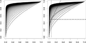
Figure 2: Left: plot of the family of curves $\{t\mapsto t^{1/(2+j/2)}\}_{j=0,\ldots,56}$ (thin solid curves). Right: choice (thick solid curve) within the family of curves $\{t\mapsto t^{1/\sigma}\}_{\sigma>1}$ that fulfills (9) and (10) for $C_{m}=1/2$ (given by the dashed horizontal line) and $\tau_{m}=2$ (slope of the dashed oblique line). This gives $\sigma_{m}\simeq 4$. The Bayes threshold $t_{m}^{B}$ is given by the dotted vertical line.

(resp., $\{2\overline{D}(\overline{D}{}^{-1}(\cdot/2)/\sigma)\}_{\sigma>1}$), $F_{m}$ is the unique curve such that the pre-image of $C_{m}$ has a tangent of slope $\tau_{m}$, that is, $f_{m}(F_{m}^{-1}(C_{m}))=\tau_{m}$. This is illustrated in Figure 2 for the Laplace scale model. In this case, $\overline{D}(x)=d(x)=e^{-x}/2$ for $x\geq 0$ and thus $F_{m}(t)=t^{1/\sigma_{m}}$, so that the family of curves is simply $\{t\mapsto t^{1/\sigma}\}_{\sigma>1}$.

Remark 2.2.

Condition (BP) constrains the model parameters to be located in a very specific region. For instance, in the Gaussian location model with $\tau_{m}=m^{\beta}$, condition (BP) implies that $\mu_{m}\sim\sqrt{2\beta\log m}$ (see Table 3 in the supplemental article NR2011supp ), which corresponds to choosing $(\mu_{m},\beta)$ on the “estimation boundary,” as displayed in Figure 1 of DJ2004 .

2.4 BFDR thresholding

Let us consider the following Bayesian quantity:

$$\mathrm{BFDR}_{m}(t)=\mathbb{P}(H_{i}=0|p_{i}\leq t)=\frac{\pi_{0,m}t}{G_{m}(t)}=\bigl{(}1+\tau_{m}^{-1}F_{m}(t)/t\bigr{)}^{-1}$$ (11)

for any $t\in(0,1)$ and where $G_{m}(t)=\pi_{0,m}t+\pi_{1,m}F_{m}(t)$. As introduced by ET2002 , the quantity defined by (11) is called “Bayesian FDR.” It is not to be confounded with “Bayes FDR” defined by SZG2008 . Also, under a two-class mixture model, $\mathrm{BFDR}_{m}(t)$ coincides with the so-called “positive false discovery rate,” itself connected to the original false discovery rate of BH1995 ; see Storey2003 and Section 4 of BCFG2010 .

Under assumption (A($F_{m},\tau_{m}$)), the function $\Psi_{m}\dvtx t\in(0,1)\mapsto F_{m}(t)/t$ is decreasing from $f_{m}(0^{+})$ to $1$, with $f_{m}(0^{+})\in(1,+\infty]$. Hence, the following result holds.

Lemma 2.3

Assume (A($F_{m},\tau_{m}$)) and $\alpha_{m}\in((1+f_{m}(0^{+})/\tau_{m})^{-1},\pi_{0,m})$. Then, equation $\mathrm{BFDR}_{m}(t)=\alpha_{m}$ has a unique solution $t=t_{m}^{\star}(\alpha_{m})\in(0,1)$, given by

$$t^{\star}_{m}(\alpha_{m})=\Psi_{m}^{-1}(q_{m}\tau_{m})$$ (12)

for $q_{m}=\alpha_{m}^{-1}-1>0$ and $\Psi_{m}(t)=F_{m}(t)/t$.

The threshold $t^{\star}_{m}(\alpha_{m})$ is called the BFDR threshold at level $\alpha_{m}$. Typically, it is well defined for any $\alpha_{m}\in(0,1/2)$, because $\pi_{0,m}>1/2$ and $f_{m}(0^{+})=+\infty$ in the Subbotin location and scale models (additionally assuming $\zeta>1$ for the location model). Obviously, the BFDR threshold is unknown because it depends on $\tau_{m}$ and on the distribution of the data. However, its interest lies in that it is close to the FDR threshold which is observable. When not ambiguous, $t^{\star}_{m}(\alpha_{m})$ will be denoted by $t^{\star}_{m}$ for short.

Next, a quantity of interest in Lemma 2.3 is $q_{m}=\alpha_{m}^{-1}-1>0$, called the recovery parameter (associated to $\alpha_{m}$). As $\alpha_{m}=(1+q_{m})^{-1}$, considering $\alpha_{m}$ or $q_{m}$ is equivalent. Since we would like to have $t^{\star}_{m}=\Psi_{m}^{-1}(q_{m}\tau_{m})$ close to $t^{B}_{m}=f_{m}^{-1}(\tau_{m})$, the recovery parameter can be interpreted as a correction factor that cancels the difference between $\Psi_{m}(t)=F_{m}(t)/t$ and $f_{m}(t)=F_{m}^{\prime}(t)$. Clearly, the best choice for the recovery parameter is such that $t^{\star}_{m}=t^{B}_{m}$, that is,

$$q_{m}^{\mathrm{opt}}=\tau_{m}^{-1}\Psi_{m}\bigl{(}f_{m}^{-1}(\tau_{m})\bigr{)}=\frac{C_{m}}{\tau_{m}t_{m}^{B}},$$ (13)

which is an unknown quantity, called the optimal recovery parameter. Note that from the concavity of $F_{m}$, we have $\Psi_{m}(t)\geq f_{m}(t)$ and thus $q_{m}^{\mathrm{opt}}\geq 1$. As an illustration, for the Laplace scale model, we have $\sigma_{m}f_{m}(t)=\Psi_{m}(t)$ and thus the optimal recovery parameter is $q_{m}^{\mathrm{opt}}=\sigma_{m}$.

The fact that $q_{m}^{\mathrm{opt}}\geq 1$ suggests to always choose $q_{m}\geq 1$ (i.e., $\alpha_{m}\leq 1/2$) into the BFDR threshold. A related result is that taking any sequence $(\alpha_{m})_{m}$ such that $\alpha_{m}\geq\alpha_{-}>1/2$ for all $m\geq 2$ never leads to an asymptotically optimal BFDR procedure; see Section 13 in the supplemental article NR2011supp .

Figure 3: Left: illustration of the FDR threshold (15): e.c.d.f. of the $p$-value (solid line), line of slope $1/\alpha_{m}$ (dotted line), the FDR threshold at level $\alpha_{m}$ ($X$-coordinate of the vertical dashed dotted line). Right: illustration of the FDR threshold as an empirical surrogate for the BFDR threshold; compared to the left picture, we added the c.d.f. of the $p$-values (thick solid line), the BFDR threshold at level $\alpha_{m}\pi_{0,m}$ (dotted vertical line) and the Bayes threshold (dashed vertical line). In both panels, we consider the Laplace scale model with $C_{m}=0.5$; $m=50$; $\beta=0.2$; $\tau_{m}=m^{\beta}$; $\sigma_{m}\simeq 4.2$; $\alpha_{m}=0.4$.

2.5 FDR thresholding

The FDR threholding procedure was introduced by Benjamini and Hochberg (1995) by proving that it controls the FDR; see BH1995 . From an historical perspective, it is interesting to note that this procedure has a prior occurrence in a series of papers by Eklund (1961–1963); see See1968 . As noted by many authors (see, e.g., Sen1999 , ET2002 , Storey2002 , GW2002 , ABDJ2006 ), this thresholding rule can be expressed as a function of the empirical c.d.f. ${\widehat{\mathbb{G}}_{m}}$ of the $p$-values in the following way: for any $\alpha_{m}\in(0,1)$,

$$\hat{t}^{\mathrm{BH}}_{m}(\alpha_{m})=\max\bigl{\{}t\in[0,1]\dvtx{\widehat{\mathbb{G}}_{m}}(t)\geq t/\alpha_{m}\bigr{\}}.$$ (14)

We simply denote $\hat{t}^{\mathrm{BH}}_{m}(\alpha_{m})$ by $\hat{t}^{\mathrm{BH}}_{m}$ when not ambiguous. Classically, this implies that $t=\hat{t}^{\mathrm{BH}}_{m}$ solves the equation ${\widehat{\mathbb{G}}_{m}}(t)=t/\alpha_{m}$ [this can be easily shown by using (14) together with the fact that ${\widehat{\mathbb{G}}_{m}}(\cdot)$ is a nondecreasing function]. Hence, according to Lemma 2.3 and as already mentioned in the literature (see BCFG2010 ), $\hat{t}^{\mathrm{BH}}_{m}$ can be seen as an empirical counterpart of the BFDR threshold at level $\alpha_{m}\pi_{0,m}$, in which the theoretical c.d.f. $G_{m}(t)=\pi_{0,m}t+\pi_{1,m}F_{m}(t)$ of the $p$-values has been replaced by the empirical c.d.f. ${\widehat{\mathbb{G}}_{m}}$ of the $p$-values. Next, once $\alpha_{m}$ has been chosen, (14) only involves observable quantities, so that the threshold $\hat{t}^{\mathrm{BH}}_{m}$ only depends on the data. This is further illustrated on the left panel of Figure 3. Also, as already observed in Section 5.2 of BCFG2010 , since the BH procedure is never more conservative than the Bonferroni procedure, the following modification of $\hat{t}^{\mathrm{BH}}_{m}$ can be proposed:

Definition 2.4.

The FDR threshold at level $\alpha_{m}$ is defined by

$$\hat{t}_{m}^{\mathrm{FDR}}(\alpha_{m})=\hat{t}^{\mathrm{BH}}_{m}(\alpha_{m})\vee(\alpha_{m}/m),$$ (15)

where $\hat{t}^{\mathrm{BH}}_{m}(\alpha_{m})$ is defined by (14).

We simply denote $\hat{t}^{\mathrm{FDR}}_{m}(\alpha_{m})$ by $\hat{t}^{\mathrm{FDR}}_{m}$ when not ambiguous. The threshold $\hat{t}^{\mathrm{FDR}}_{m}$ is the one that we use throughout this paper. This modification does not change the risk $R^{T}_{m}(\cdot)$, that is, $R^{T}_{m}(\hat{t}^{\mathrm{BH}}_{m})=R_{m}^{T}(\hat{t}_{m}^{\mathrm{FDR}})$, but can affect the risk $R^{I}_{m}(\cdot)$, that is, $R^{I}_{m}(\hat{t}^{\mathrm{BH}}_{m})\neq R^{I}_{m}(\hat{t}_{m}^{\mathrm{FDR}})$, in general.

Finally, while relation (15) uses $p$-values whereas the algorithms defined in Section 1.3 use test statistics, it is easy to check that the resulting procedures are the same.

Remark 2.5 ((Adaptive FDR procedures under sparsity)).

To get a better FDR controlling procedure, one classical approach is to modify (15) by dividing $\alpha_{m}$ by a (more or less explicit) estimator of $\pi_{0,m}$ and by possibly using a step-up-down algorithm; see, for example, TLD1998 , Sar2002 , BKY2006 , Sar2008 , BR2009 , FDR2009 , GBS2009 . However, this method seems not helpful in our sparse setting because $\pi_{0,m}$ is very close to $1$. As a result, we focus in this paper only on the original (nonadaptive) version of FDR thresholding (15).

3 Results in the general model

This section presents relations of the form (5) and (6) for the BFDR and FDR thresholds. Our first main result deals with the BFDR threshold.

Theorem 3.1

Assume (A($F_{m},\tau_{m}$)) and consider the BFDR threshold $t_{m}^{\star}$ at a level $\alpha_{m}\in((1+f_{m}(0^{+})/\tau_{m})^{-1},\pi_{0,m})$ corresponding to a recovery parameter $q_{m}=\alpha_{m}^{-1}-1$. Consider $q_{m}^{\mathrm{opt}}\geq 1$ the optimal recovery parameter given by (13). Then the following holds: [(ii)]

if $\alpha_{m}\leq 1/2$, we have for any $m\geq 2$,

$$R_{m}\bigl{(}t_{m}^{\star}\bigr{)}-R_{m}\bigl{(}t_{m}^{B}\bigr{)}\leq\pi_{1,m}\bigl{\{}\bigl{(}C_{m}/q_{m}-C_{m}/q_{m}^{\mathrm{opt}}\bigr{)}\vee\gamma_{m}\bigr{\}},$$ (16)

where we let $\gamma_{m}=(C_{m}-F_{m}(\Psi_{m}^{-1}(q_{m}\tau_{m})))_{+}$.

In particular, under (BP), if $\alpha_{m}\rightarrow 0$ and $\gamma_{m}\rightarrow 0$, the BFDR threshold $t_{m}^{\star}$ is asymptotically optimal at rate $\rho_{m}=\alpha_{m}+\gamma_{m}$.

we have for any $m\geq 2$,

$$\frac{R_{m}(t_{m}^{\star})}{R_{m}(t_{m}^{B})}\geq\frac{\pi_{1,m}}{R_{m}(t_{m}^{B})}\bigl{(}1-\bigl{(}1-q_{m}^{-1}\bigr{)}_{+}F_{m}\bigl{(}q_{m}^{-1}\tau_{m}^{-1}\bigr{)}\bigr{)}.$$ (17)

In particular, under (BP), if $R_{m}(t_{m}^{B})\sim\pi_{1,m}(1-C_{m})$ and if $q_{m}$ is chosen such that

$$\liminf_{m}\biggl{\{}\frac{1-(1-q_{m}^{-1})_{+}F_{m}(q_{m}^{-1}\tau_{m}^{-1})}{1-C_{m}}\biggr{\}}>1,$$ (18)

$t_{m}^{\star}$ is not asymptotically optimal.

Theorem 3.1 is proved in Section 7. Theorem 3.1(i) presents an upper-bound for the excess risk when choosing $q_{m}$ instead of $q_{m}^{\mathrm{opt}}$ in BFDR thresholding. First, both sides of (16) are equal to zero when $q_{m}=q_{m}^{\mathrm{opt}}$. Hence, this bound is sharp in that case. Second, assumption “$\alpha_{m}\leq 1/2$” in Theorem 3.1(i) is only a technical detail that allows us to get $C_{m}/q_{m}$ instead of $1/q_{m}$ in the right-hand side of (16) (moreover, it is quite natural; see the end of Section 2.4). Third, $\gamma_{m}$ has a simple interpretation as the difference between the power of Bayes’ thresholding and BFDR thresholding. Fourth, bound (16) induces the following trade-off for choosing $\alpha_{m}$: on the one hand, $\alpha_{m}$ has to be chosen small enough to make $C_{m}/q_{m}$ small; on the other hand, $\gamma_{m}$ increases as $\alpha_{m}$ decreases to zero. Finally note that, in Theorem 3.1(i), the second statement is a consequence of the first one because $R_{m}(t_{m}^{B})\geq\pi_{1,m}(1-C_{m})$. Theorem 3.1(ii) states lower bounds which are useful to identify regimes of $\alpha_{m}$ that do not lead to an asymptotically optimal BFDR thresholding; see Corollary 4.4(i) further on.

Our second main result deals with FDR thresholding.

Theorem 3.2

Let $\varepsilon\in(0,1)$, assume (A($F_{m},\tau_{m}$)) and consider the FDR threshold $\hat{t}^{\mathrm{FDR}}_{m}$ at level $\alpha_{m}>(1-\varepsilon)^{-1}(\pi_{0,m}+\pi_{1,m}f_{m}(0^{+}))^{-1}$. Then the following holds: for any $m\geq 2$,

$$R_{m}\bigl{(}\hat{t}^{\mathrm{FDR}}_{m}\bigr{)}-R_{m}\bigl{(}t_{m}^{B}\bigr{)} \leq \pi_{1,m}\frac{\alpha_{m}}{1-\alpha_{m}}+m^{-1}\frac{\alpha_{m}}{(1-\alpha_{m})^{2}}$$

$${}+\pi_{1,m}\bigl{\{}\gamma^{\prime}_{m}\wedge\bigl{(}\gamma_{m}^{\varepsilon}+e^{-m\varepsilon^{2}(\tau_{m}+1)^{-1}(C_{m}-\gamma_{m}^{\varepsilon})/4}\bigr{)}\bigr{\}}$$

for $\gamma^{\varepsilon}_{m}=(C_{m}-F_{m}(\Psi_{m}^{-1}(q_{m}^{\varepsilon}\tau_{m})))_{+}$ with $q_{m}^{\varepsilon}=(\alpha_{m}\pi_{0,m}(1-\varepsilon))^{-1}-1$ and $\gamma^{\prime}_{m}=(C_{m}-F_{m}(\alpha_{m}/m))_{+}$. In particular, under (BP) and assuming $\alpha_{m}\rightarrow 0$:

[(ii)]

if $m/\tau_{m}\rightarrow+\infty$, $\gamma_{m}^{\varepsilon}\rightarrow 0$ and additionally $\forall\kappa>0$, $e^{-\kappa m/\tau_{m}}=o(\gamma^{\varepsilon}_{m})$, the FDR threshold $\hat{t}^{\mathrm{FDR}}_{m}$ is asymptotically optimal at rate $\rho_{m}=\alpha_{m}+\gamma_{m}^{\varepsilon}$;

if $m/\tau_{m}\rightarrow\ell\in(0,+\infty)$ with $\gamma^{\prime}_{m}\rightarrow 0$, the FDR threshold $\hat{t}^{\mathrm{FDR}}_{m}$ is asymptotically optimal at rate $\rho_{m}=\alpha_{m}+\gamma^{\prime}_{m}$.

Theorem 3.2 is proved in Section 7. The proof mainly follows the methodology of BCFG2010 , but is more general and concise. It relies on tools developed in FR2002 , GW2002 , FZ2006 , FDR2009 , RV2010 , Roq2011 . The main argument for the proof is that the FDR threshold $\hat{t}^{\mathrm{FDR}}_{m}(\alpha_{m})$ is either well concentrated around the BFDR threshold ${t}^{\star}_{m}(\alpha_{m}\pi_{0,m})$ (as illustrated in the right panel of Figure 3) or close to the Bonferroni threshold $\alpha_{m}/m$. This argument was already used in BCFG2010 .

Let us comment briefly on Theorem 3.2: first, as in the BFDR case, choosing $\alpha_{m}$ such that the bound in (3.2) is minimal involves a trade-off because $\gamma_{m}^{\varepsilon}$ and $\gamma^{\prime}_{m}$ are quantities that increase when $\alpha_{m}$ decreases to zero. Second, let us note that cases (i) and (ii) in Theorem 3.2 are intended to cover regimes where the FDR is close to BFDR (moderately sparse) and where the FDR threshold is close to the Bonferroni threshold (extremely sparse), respectively. In particular, these two regimes cover the case where $\tau_{m}=m^{\beta}$ with $\beta\in(0,1]$. Finally, the bounds and convergence rates derived in Theorems 3.1 and 3.2 strongly depend on the nature of $F_{m}$. We derive a more explicit expression of the latter in the next section, in the particular cases of location and scale models coming from a Subbotin density.

Remark 3.3 ((Conservative upper-bound for $\gamma_{m}$)).

By the concavity of $F_{m}$, we have $q_{m}\tau_{m}=\Psi_{m}(t_{m}^{\star})\geq f_{m}(t_{m}^{\star})$, which yields

$$\gamma_{m}\leq C_{m}-F_{m}\bigl{(}f_{m}^{-1}(q_{m}\tau_{m})\bigr{)}\in[0,1).$$ (20)

When $f_{m}^{-1}$ is easier to use than $\Psi_{m}^{-1}$, it is tempting to use (20) to upper bound the excess risk in Theorems 3.1 and 3.2. However, this can inflate the resulting upper-bound too much. This point is discussed in Section 10.4 in the supplemental article NR2011supp for the case of a Gaussian density (for which this results in an additional $\log\log\tau_{m}$ factor in the bound).

4 Application to location and scale models

4.1 The Bayes risk and optimal recovery parameter

A preliminary task is to study the behavior of $t_{m}^{B}$, $R_{m}(t^{B}_{m})$ and $q_{m}^{\mathrm{opt}}=C_{m}/(\tau_{m}t_{m}^{B})$ both in location and scale models. While finite sample inequalities are given in Section 9.2 in the supplemental article NR2011supp , we only report in this subsection some resulting asymptotic relations for short. Let us define the following rates, which will be useful throughout the paper:

$$r^{\mathrm{loc}}_{m} = \bigl{(}\zeta\log\tau_{m}+\bigl{|}\overline{D}{}^{-1}(C_{m})\bigr{|}^{\zeta}\bigr{)}^{1-1/\zeta};$$ (21)

$$r^{\mathrm{sc}}_{m} = \zeta\log\tau_{m}+\bigl{(}\overline{D}{}^{-1}(C_{m}/2)\bigr{)}^{\zeta}.$$ (22)

Under (Sp), note that the rates $r^{\mathrm{loc}}_{m}$ (resp., $r^{\mathrm{sc}}_{m}$) tend to infinity. Furthermore, by using Section 9.2 in the supplemental article NR2011supp , we have $\mu_{m}=(r^{\mathrm{loc}}_{m})^{1/(\zeta-1)}-\overline{D}{}^{-1}(C_{m})$ in the location model and $\sigma_{m}\geq(r^{\mathrm{sc}}_{m})^{1/\zeta}/(\overline{D}{}^{-1}(C_{m}/2))$ in the scale model.

Proposition 4.1

Consider a $\zeta$-Subbotin density (4) with $\zeta\geq 1$ for a scale model and $\zeta>1$ for a location model. Let $(\tau_{m},C_{m})\in(1,\infty)\times(0,1)$ be the parameters of the model. Let $r_{m}$ be equal to $r^{\mathrm{loc}}_{m}$ defined by (21) in the location model or to $r^{\mathrm{sc}}_{m}$ defined by (22) in the scale model. Then, under (BP) and (Sp), we have $\mu_{m}\sim r^{\mathrm{loc}}_{m}\sim(\zeta\log\tau_{m})^{1/\zeta}$ and $\sigma_{m}\sim(r^{\mathrm{sc}}_{m})^{1/\zeta}/(\overline{D}{}^{-1}(C_{m}/2))\sim(\zeta\log\tau_{m})^{1/\zeta}/(\overline{D}{}^{-1}(C_{m}/2))$ and

$$R_{m}\bigl{(}t_{m}^{B}\bigr{)} \sim \pi_{1,m}(1-C_{m}),$$ (23)

$$t^{B}_{m} = O\bigl{(}R_{m}\bigl{(}t_{m}^{B}\bigr{)}/r_{m}\bigr{)},$$ (24)

$$q_{m}^{\mathrm{opt}} \sim \cases{\displaystyle\frac{C_{m}}{d(\overline{D}{}^{-1}(C_{m}))}(\zeta\log\tau_{m})^{1-1/\zeta}&\quad(location),\vspace*{2pt}\cr\displaystyle\frac{C_{m}/2}{\overline{D}{}^{-1}(C_{m}/2)d(\overline{D}{}^{-1}(C_{m}/2))}\zeta\log\tau_{m}&\quad(scale).}$$ (25)

From (23) and (24), by assuming (BP) and (Sp), the probability of a type I error ($\pi_{0,m}t_{m}^{B}$) is always of smaller order than the probability of a type II error ($\pi_{1,m}(1-C_{m})$). The latter had already been observed in BCFG2010 in the particular case of a Gaussian scale model.

Remark 4.2.

From (23) and since the risk of null thresholding is $R_{m}(0)=\pi_{1,m}$, a substantial improvement over the null threshold can only be expected in the regime where $C_{m}\geq C_{-}$, where $C_{-}$ is “far” from $0$.

4.2 Finite sample oracle inequalities

The following result can be derived from Theorem 3.1(i) and Theorem 3.2. It is proved in Section 9.3 in the supplemental article NR2011supp .

Corollary 4.3

Consider a $\zeta$-Subbotin density (4) with $\zeta>1$ for a location model and $\zeta\geq 1$ for a scale model, and let $(\tau_{m},C_{m})\in(1,\infty)\times(0,1)$ be the parameters of the model. Let $r_{m}=r^{\mathrm{loc}}_{m}$ [defined by (21)] and $K_{m}=d(0)$ in the location model or $r_{m}=r^{\mathrm{sc}}_{m}$ [defined by (22)] and $K_{m}=2\overline{D}{}^{-1}(C_{m}/2)d(\overline{D}{}^{-1}(C_{m}/2))$ in the scale model. Let $\alpha_{m}\in(0,1/2)$ and denote the corresponding recovery parameter by $q_{m}=\alpha_{m}^{-1}-1$. Consider $q_{m}^{\mathrm{opt}}\geq 1$ the optimal recovery parameter given by (13). Let $\nu\in(0,1)$. Then: [(ii)]

The BFDR threshold $t_{m}^{\star}$ at level $\alpha_{m}$ defined by (12) satisfies that for any $m\geq 2$ such that $r_{m}\geq\frac{K_{m}}{C_{m}(1-\nu)}(\log(q_{m}/q_{m}^{\mathrm{opt}})-\log\nu)$,

$$R_{m}\bigl{(}t_{m}^{\star}\bigr{)}-R_{m}\bigl{(}t_{m}^{B}\bigr{)}$$

(26)

$$\qquad\leq\pi_{1,m}\biggl{\{}\biggl{(}\frac{C_{m}}{q_{m}}-\frac{C_{m}}{q_{m}^{\mathrm{opt}}}\biggr{)}\vee\biggl{(}K_{m}\frac{\log(q_{m}/q_{m}^{\mathrm{opt}})-\log\nu}{r_{m}}\biggr{)}\biggr{\}}.$$

Letting $\varepsilon\in(0,1)$, $D_{1,m}=-\log(\nu\pi_{0,m}(1-\varepsilon))$ and $D_{2,m}=\log(\nu^{-1}\*C_{m}\tau_{m}^{-1}m)$, the FDR threshold $\hat{t}^{\mathrm{FDR}}_{m}$ at level $\alpha_{m}$ defined by (15) satisfies that, for any $a\in\{1,2\}$, for any $m\geq 2$ such that $r_{m}\geq\frac{K_{m}}{C_{m}(1-\nu)}(\log(\alpha_{m}^{-1}/q_{m}^{\mathrm{opt}})+D_{a,m})$,

$$\qquad R_{m}\bigl{(}\hat{t}^{\mathrm{FDR}}_{m}\bigr{)}-R_{m}\bigl{(}t_{m}^{B}\bigr{)} \leq \pi_{1,m}\biggl{(}\frac{\alpha_{m}}{1-\alpha_{m}}+K_{m}\frac{(\log(\alpha_{m}^{-1}/q_{m}^{\mathrm{opt}})+D_{a,m})_{+}}{r_{m}}\biggr{)}$$

$${}+\frac{\alpha_{m}/m}{(1-\alpha_{m})^{2}}+\pi_{1,m}{\mathbf{1}\{a=1\}}e^{-m(\tau_{m}+1)^{-1}\nu\varepsilon^{2}C_{m}/4}.$$

Corollary 4.3(ii) contains two distinct cases. The case $a=1$ should be used when $m/\tau_{m}$ is large, because the remainder term containing the exponential becomes small (whereas $D_{1,m}$ is approximately constant). The case $a=2$ is intended to deal with the regime where $m/\tau_{m}$ is not large, because $D_{2,m}$ is of the order of a constant in that case. The finite sample oracle inequalities (4.3) and (4.3) are useful to derive explicit rates of convergence, as we will see in the next section. Let us also mention that an exact computation of the excess risk of BFDR thresholding can be derived in the Laplace case; see Section 10.2 in the supplemental article NR2011supp .

4.3 Asymptotic optimality with rates

In this section, we provide a sufficient condition on $\alpha_{m}$ such that, under (BP) and (Sp), BFDR/FDR thresholding is asymptotically optimal [according to (6)], and we provide an explicit rate $\rho_{m}$. Furthermore, we establish that this condition is necessary for the optimality of BFDR thresholding.

Corollary 4.4

Take $\zeta>1$, $\gamma=1-\zeta^{-1}$ for the location case and $\zeta\geq 1$, $\gamma=1$ for the scale case. Consider a $\zeta$-Subbotin density (4) in the sparsity regime $\tau_{m}=m^{\beta}$, $0<\beta\leq 1$ and under (BP). Then the following holds: [(iii)]

The BFDR threshold $t_{m}^{\star}$ is asymptotically optimal if and only if

$$\alpha_{m}\rightarrow 0\quad\mbox{and}\quad\log\alpha_{m}=o\bigl{(}(\log m)^{\gamma}\bigr{)},$$ (28)

in which case it is asymptotically optimal at rate $\rho_{m}=\alpha_{m}+\frac{(\log(\alpha_{m}^{-1}/(\log m)^{\gamma}))_{+}}{(\log m)^{\gamma}}.$

The FDR threshold $\hat{t}^{\mathrm{FDR}}_{m}$ at a level $\alpha_{m}$ satisfying (28) is asymptotically optimal at rate $\rho_{m}=\alpha_{m}+\frac{(\log(\alpha_{m}^{-1}/(\log m)^{\gamma}))_{+}}{(\log m)^{\gamma}}$.

Choosing $\alpha_{m}\propto 1/(\log m)^{\gamma}$, BFDR and FDR thresholding are both asymptotically optimal at rate $\rho_{m}=1/(\log m)^{\gamma}$.

In the particular case of a Gaussian scale model $(\zeta=2)$, Corollary 4.4 recovers Corollaries 4.2 and 5.1 of BCFG2010 . Corollary 4.4 additionally provides a rate, and encompasses the location case and other values of $\zeta$.

Remark 4.5 ((Lower bound for the Laplace scale model)).

We can legitimately ask whether the rate $\rho_{m}=(\log m)^{-\gamma}$ can be improved. We show that this rate is the smallest that one can obtain over a sparsity class $\beta\in[\beta_{-},1]$ for some $\beta_{-}\in(0,1)$, in the particular case of BFDR thresholding and in the Laplace scale model; see Corollary 10.2 in the supplemental article NR2011supp . While the calculations become significantly more difficult in the other models, we believe that the minimal rate for the relative excess risk of the BFDR is still $(\log m)^{-\gamma}$ in a Subbotin location and scale models. Also, since the FDR can be seen as a stochastic variation around the BFDR, we may conjecture that this rate is also minimal for FDR thresholding.

4.4 Choosing $\alpha_{m}$

Let us consider the sparsity regime $\tau_{m}=m^{\beta}$, $\beta\in(0,1)$. Corollary 4.4 suggests to choose $\alpha_{m}$ such that $\alpha_{m}\propto(\log m)^{-\gamma}$. This is in accordance with the recommendation of BCFG2010 in the Gaussian scale model; see Remark 5.3 therein. In this section, we propose an explicit choice of $\alpha_{m}$ from an priori value $(\beta_{0},C_{0})$ of the unknown parameter $(\beta,C_{m})$.

Let us choose a value $(\beta_{0},C_{0})$ a priori for $(\beta,C_{m})$. A natural choice for $\alpha_{m}$ is the value which would be optimal if the parameters of the model were $(\beta,C_{m})=(\beta_{0},C_{0})$. Namely, by using (13) in Section 2.4, we choose $\alpha_{m}=\alpha_{m}^{\mathrm{opt}}(\beta_{0},C_{0})$, where

$$\alpha_{m}^{\mathrm{opt}}(\beta_{0},C_{0})=\bigl{(}1+q_{m}^{\mathrm{opt}}(\beta_{0},C_{0})\bigr{)}^{-1}$$ (30)

$$\eqntext{\mbox{with $q_{m}^{\mathrm{opt}}(\beta_{0},C_{0})=m^{-\beta_{0}}C_{0}/F_{m,0}^{-1}(C_{0})$}}$$

by denoting $F_{m,0}$ the c.d.f. of the $p$-values following the alternative for the model parameters $(\beta_{0},C_{0})$. For instance:

• [-]

• Gaussian location: $F_{m,0}^{-1}(C_{0})=\overline{\Phi}(\{\overline{\Phi}{}^{-1}(C_{0})^{2}+2\beta_{0}\log m\}^{1/2})$;

• Gaussian scale: $F_{m,0}^{-1}(C_{0})=2\overline{\Phi}(\overline{\Phi}{}^{-1}(C_{0}/2)x)$, where $x>1$ is the solution of $2\beta_{0}\log m+2\log x=(\overline{\Phi}{}^{-1}(C_{0}/2))^{2}(x^{2}-1)$;

• Laplace scale: $q_{m}^{\mathrm{opt}}(\beta_{0},C_{0})=y$, where $y>1$ is the solution of $\beta_{0}\log m+\log y=(y-1)\log(1/C_{0})$,

where $\overline{\Phi}(z)$ denotes $\mathbb{P}(Z\geq z)$ for $Z\sim\mathcal{N}(0,1)$.

The above choice of $\alpha_{m}$ does depend on $(\beta_{0},C_{0})$, which can be interpreted as a “guess” on the value of the unknown parameter $(\beta,C_{m})$. Hence, when no prior information on $(\beta,C_{m})$ is available from the data, the above choice of $\alpha_{m}$ can appear of limited interest in practice. However, we would like to make the following two points:

• asymptotically, choosing $\alpha_{m}=\alpha_{m}^{\mathrm{opt}}(\beta_{0},C_{0})$ always yields an optimal(B)FDR thresholding [under (BP)], even if $(\beta_{0},C_{0})\neq(\beta,C_{m})$: by Proposition 4.1, we get $\alpha_{m}^{\mathrm{opt}}(\beta_{0},C_{0})\propto(\log m)^{-\gamma}$ and thus the asymptotic optimality is a direct consequence of Corollary 4.4(iii);

• nonasymptotically, our numerical experiments suggest that $\alpha_{m}=\break\alpha_{m}^{\mathrm{opt}}(\beta_{0},C_{0})$ performs fairly well when we have at hand an a priori on the location of the model parameters: if $(\beta,C_{m})$ is supposed to be in some specific (but possibly large) region of the “sparsity${}\times{}$power” square, choosing any $(\beta_{0},C_{0})$ in that region yields a thresholding procedure with a reasonably small risk; see Sections 5 and 14 in the supplemental article NR2011supp .

Finally, let us note that the choice $\alpha_{m}=\alpha_{m}^{\mathrm{opt}}(\beta_{0},C_{0})$ is motivated by the analysis of the BFDR risk, not that of the FDR risk. Hence, it might be possible to choose a better $\alpha_{m}$ for FDR thresholding, especially for small values of $m$ for which BFDR and FDR are different. Because obtaining such a refinement appeared quite challenging, and as our proposed choice already performed well, we decided not to investigate this question further.

Remark 4.6.

By choosing $\alpha_{m}=\alpha_{m}^{\mathrm{opt}}(\beta_{0},C_{0})$ as in (30), we can legitimately ask how large the constants are in the finite sample inequalities coming from Corollary 4.3 in standard cases. To simplify the problem, let us focus on the BFDR threshold and consider a $\zeta$-Subbotin location model with $\zeta>1$. Taking $\tau_{m}=m^{\beta}$, the parameters of the model are $(\beta,C_{m})\in(0,1]\times(0,1)$. Assume that the parameter sequence $(C_{m})_{m}$ satisfies (BP) for some $0<C_{-}\leq C_{+}<1$. Then Corollary 9.4 in the supplemental article NR2011supp provides explicit constants $D=D(\beta,C_{-},C_{+},\beta_{0},C_{0},\nu)$ and $M=M(\beta,C_{-},C_{+},\beta_{0},C_{0},\nu)$ such that the following inequality holds:

$$\qquad\bigl{(}R_{m}\bigl{(}t_{m}^{\star}\bigr{)}-R_{m}\bigl{(}t_{m}^{B}\bigr{)}\bigr{)}/R_{m}\bigl{(}t_{m}^{B}\bigr{)}\leq D/(\log m)^{1-1/\zeta}\qquad\mbox{for any $m\geq M$.}$$ (31)

As an illustration, in the Gaussian case ($\zeta=2$), for $\beta=0.7$, $C_{-}=0.5$, $C_{+}=0.7$, $\beta_{0}=C_{0}=0.5$ and $\nu=0.25$, we have $M\simeq 61.6$ and $D\simeq 2.66$. As expected, these constants are over-estimated: for instance, by taking $m=1000$, the left-hand side of (31) is smaller than $0.1$ (see Figure 4 in the next section) while the right-hand side of (31) is $D/\sqrt{\log(1000)}\simeq 1.01$. Finally, we can check that $D$ becomes large when $\beta$ is close to $0$ or $C_{+}$ is close to $1$. These configurations correspond to the cases where the data are almost nonsparse and where the Bayes rule can have almost full power, respectively. They can be seen as limit cases for our methodology.

Remark 4.7.

By using Proposition 4.1, as $m\to+\infty$, $\alpha_{m}^{\mathrm{opt}}(\beta_{0},C_{0})\sim\alpha_{m}^{\infty}(\beta_{0},C_{0})$, for an equivalent $\alpha_{m}^{\infty}(\beta_{0},C_{0})$ having a very simple form; see Section 10.1 in the supplemental article NR2011supp . Therefore, we could use $\alpha_{m}^{\infty}(\beta_{0},C_{0})$ instead of $\alpha_{m}^{\mathrm{opt}}(\beta_{0},C_{0})$. Numerical comparisons between the (B)FDR risk obtained according to $\alpha_{m}^{\mathrm{opt}}(\beta_{0},C_{0})$ and $\alpha_{m}^{\infty}(\beta_{0},C_{0})$ are provided in Section 14 in the supplemental article NR2011supp . While $\alpha_{m}^{\infty}(\beta_{0},C_{0})$ qualitatively leads to the same results when $m$ is large (say, $m\geq 1000$), the use of $\alpha_{m}^{\mathrm{opt}}(\beta_{0},C_{0})$ is more accurate for a small $m$.

5 Numerical experiments

In order to complement the convergence results stated above, it is of interest to study the behavior of FDR and BFDR thresholding for a small or moderate $m$ in numerical experiments. These experiments have been performed for the inductive risk $R_{m}(\cdot)=R^{I}_{m}(\cdot)$ defined by (8).

5.1 Exact formula for the FDR risk

The BFDR threshold $t_{m}^{\star}$ can be approximated numerically, which allows us to compute $R_{m}(t_{m}^{\star})$. Computing $R_{m}(\hat{t}^{\mathrm{FDR}}_{m})$ is more complicated because the FDR threshold $\hat{t}^{\mathrm{FDR}}_{m}$ is not deterministic. However, we can avoid performing cumbersome and somewhat imprecise simulations to compute

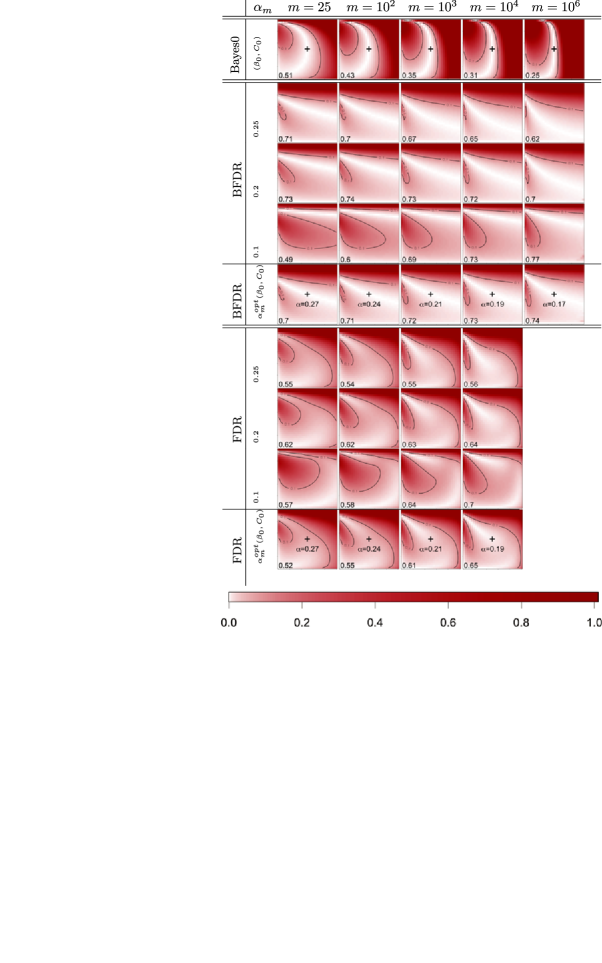
Figure 4: Adaptation to sparsity by (B)FDR thresholding in the Gaussian location model relative excess risks $\mathcal{E}_{m}$ for various thresholding procedures (rows) and different values of $m$ (columns). In each panel, the corresponding risk is plotted as a function of $\beta\in[0,1]$ (horizontal axis) and $C_{m}\in[0,1]$ (vertical axis). Colors range from white (low risk) to dark red (high risk), as indicated by the color bar at the bottom. Black lines represent the level set $\mathcal{E}_{m}=0.1$. The point $(\beta,C_{m})=(\beta_{0},C_{0})$ is marked by “$+$.” We chose $\beta_{0}=1/2$ and $C_{0}=1/2$. See main text for details.

$R_{m}(\hat{t}^{\mathrm{FDR}}_{m})$ by using the approach proposed in FR2002 and RV2010 . Using this methodology, the full distribution of $\hat{t}^{\mathrm{FDR}}_{m}$ may be written as a function of the joint c.d.f. of the order statistics of i.i.d. uniform variables. Let for any $k\geq 0$ and for any $(t_{1},\ldots,t_{k})\in[0,1]^{k}$, $\Psi_{k}(t_{1},\ldots,t_{k})=\mathbb{P}(U_{(1)}\leq t_{1},\ldots,U_{(k)}\leq t_{k}),$ where $(U_{i})_{1\leq i\leq k}$ is a sequence of i.i.d. uniform variables on $(0,1)$ and with the convention $\Psi_{0}(\cdot)=1$. The $\Psi_{k}$’s can be evaluated, for example, by using Steck’s recursion; see SW1986 , pages 366–369. Then, relation (10) in RV2010 entails

$$R_{m}\bigl{(}\hat{t}^{\mathrm{FDR}}_{m}\bigr{)} = \sum_{k=0}^{m}\pmatrix{m\cr k}R_{m}\biggl{(}\frac{\alpha(k\vee 1)}{m}\biggr{)}G_{m}(\alpha k/m)^{k}$$

$$\hskip 14.0pt{}\times\Psi_{m-k}\bigl{(}1-G_{m}(\alpha m/m),\ldots,1-G_{m}\bigl{(}\alpha(k+1)/m\bigr{)}\bigr{)},$$

where $G_{m}(t)=\pi_{0,m}t+\pi_{1,m}F_{m}(t)$. For reasonably large $m$ ($m\leq 10\mbox{,}000$ in what follows), expression (5.1) can be used for computing the exact risk of FDR thresholding $\hat{t}^{\mathrm{FDR}}_{m}$ in our experiment.

5.2 Adaptation to unknown sparsity

We quantify the quality of a thresholding procedure using the relative excess risk

$$\mathcal{E}_{m}(\hat{t}_{m})=\bigl{(}R_{m}(\hat{t}_{m})-R_{m}\bigl{(}t^{B}_{m}\bigr{)}\bigr{)}/R_{m}\bigl{(}t^{B}_{m}\bigr{)}.$$

The closer the relative excess risk $\mathcal{E}_{m}(\hat{t}_{m})$ is to $0$, the better the corresponding classification procedure is.

Figure 4 compares relative excess risks of different procedures in the Gaussian location model (results for the Gaussian scale and the Laplace scale models are qualitatively similar, see Figures 5 and 6 in the supplemental article NR2011supp ). Each row of plots corresponds to a particular procedure, and each column to a particular value of $m\in\{25,10^{2},10^{3},10^{4},10^{5},10^{6}\}$. The first row corresponds to the Bayes procedure defined by (9), where the model parameters are taken as $(\beta,C_{m})=(\beta_{0},C_{0})$. It is denoted by Bayes0. Next, we consider BFDR (rows 2 to 5) and FDR (rows 6 to 9) thresholding at level $\alpha_{m}$, for $\alpha_{m}\in\{0.1,0.2,0.25\}$ (independent of $m$) and for the choice $\alpha_{m}=\alpha_{m}^{\mathrm{opt}}(\beta_{0},C_{0})$ defined in Section 4.4. For each procedure and each value of $m$, the behavior of the relative excess risk is studied as the (unknown) true model parameters $(\beta,C_{m})$ vary in $[0,1]\times[0,1]$, and we arbitrarily choose $\beta_{0}$ and $C_{0}$ as the midpoints of the corresponding intervals, that is, $(\beta_{0},C_{0})=(1/2,1/2)$ (similar results are obtained for other values of $(\beta_{0},C_{0})$; see Figures 8, 9 and 10 in the supplemental article NR2011supp ). Colors reflect the value of the relative excess risk. They range from white [$R_{m}=R_{m}(t^{B}_{m})$] to dark red [$R_{m}\geq 2R_{m}(t^{B}_{m})$]. Black lines represent the level set $\mathcal{E}_{m}=0.1$, that is, they delineate a region of the $(\beta,C_{m})$ plane in which the excess risk of the procedure under study is ten times less than the Bayes risk. The number at the bottom left of each plot gives the fraction of configurations $(\beta,C_{m})$ for which $\mathcal{E}_{m}\leq 0.1$. This evaluates the quality of a procedure uniformly across all the $(\beta,C_{m})$ values.

For $m=10^{6}$, we did not undertake exact FDR risk calculations: they were too computationally intensive, as the complexity of the calculation of function $\Psi_{k}$ used in (5.1) is quadratic in $m$. However, FDR risk is expected to be well approximated by BFDR risk for such a large value of $m$, as confirmed by the fact that FDR and BFDR plots at a given level $\alpha$ are increasingly similar as $m$ increases.

Bayes0 performs well when the sparsity parameter $\beta$ is correctly specified, and its performance is fairly robust to $C_{m}$. However, it performs poorly when $\beta$ is misspecified, and increasingly so as $m$ increases. The results are markedly different for the other thresholding methods. BFDR thresholding and FDR thresholding are less adaptive to $C_{m}$ than Bayes0, but much more adaptive to the sparsity parameter $\beta$, as illustrated by the fact that the configurations with low relative excess risk span the whole range of $\beta$.

For $\alpha_{m}=\alpha_{m}^{\mathrm{opt}}(\beta_{0},C_{0})$, the fraction of configurations $(\beta,C_{m})$ for which $\mathcal{E}_{m}\leq 0.1$ increases as $m$ increases. This illustrates the asymptotic optimality of (B)FDR thresholding, as stated in Corollary 4.4(iii), because $\alpha_{m}^{\mathrm{opt}}(\beta_{0},C_{0})\propto(\log m)^{-1/2}$. Additionally, observe that the $(\beta,C_{m})$-region around $(\beta_{0},C_{0})$ contains only very small values of $\mathcal{E}_{m}$, even for moderate $m$. This suggests that, nonasymptotically, $\alpha_{m}^{\mathrm{opt}}(\beta_{0},C_{0})$ is a reasonable choice for $\alpha_{m}$, when we know a priori that the parameters lie in some specific region of the $(\beta,C_{m})$-square.

Next, let us consider the case of (B)FDR thresholding using a fixed value of $\alpha_{m}=\alpha$. While our theoretical results show that choosing $\alpha_{m}$ fixed with $m$ (and in particular not tending to zero) is always asymptotically sub-optimal, the results shown by Figure 4 are less clear-cut. An explanation is that $(\log m)^{-1/2}$ decreases only slowly to zero [e.g., $\alpha_{m}^{\mathrm{opt}}(\beta_{0},C_{0})\simeq 0.17$ for $m=10^{6}$], hence the asymptotic is quite “far” and not fully attained by our experiments.

Hence, from a more practical point of view, in a classical situation where $m$ does not exceed, say, $10^{6}$, a practitioner willing to use the (B)FDR can consider two different approaches to calibrate $\alpha_{m}$: the first one is to take some arbitrary value, for example, $0.05$, $0.1$ or $0.2$. The overall excess risk might be small, but the location of the region of smallest excess risk (pictured in white in our figures) is unknown, and depends strongly on $\alpha$ and $m$ (and even $\zeta$). In contrast, the second method $\alpha_{m}^{\mathrm{opt}}(\beta_{0},C_{0})$ “stabilizes” the region of the $(\beta,C_{m})$-square where the (B)FDR has good performance across all the values of $m$ (and $\zeta$). Thus, while the first method has a clear interpretation in terms of FDR, the second approach is more interpretable w.r.t. the sparsity and power parameters and is recommended when these parameters are felt to correctly parametrize the model.

Finally note that, when considering the weighted mis-classification risk (as formally defined in (34) and studied in Section 11 in the supplemental article NR2011supp ), there exists a particular choice of the weight (as a function of $m$) such that the optimal (B)FDR level $\alpha_{m}^{\mathrm{opt}}(\beta_{0},C_{0})$ does not depend on $m$, making (B)FDR thresholding with fixed values of $\alpha_{m}$ asymptotically optimal, as noted by BCFG2010 . This point is discussed in Section 6.2.

6 Discussion

6.1 Asymptotic minimaxity over a sparsity class

Let us consider the sparsity range $\tau_{m}=m^{\beta}$, with $\beta_{-}\leq\beta\leq 1$, for some given $\beta_{-}\in(0,1)$. Assume (BP) with $C_{-}$ and $C_{+}$ defined therein. Denote the set $[\beta_{-},1]\times[C_{-},C_{+}]$ by $\Theta$ for short. The minimax risk is defined by

$$R_{m}^{\star}=\inf_{\hat{t}_{m}}\Bigl{\{}\sup_{(\beta,C_{m})\in\Theta}\bigl{\{}R_{m}(\hat{t}_{m})\bigr{\}}\Bigr{\}},$$

where the infimum is taken over the set of thresholds that can be written as measurable functions of the $p$-values. Obviously, $R_{m}^{\star}\geq\sup_{(\beta,C_{m})\in\Theta}\{R_{m}({t}_{m}^{B})\}$, where ${t}_{m}^{B}$ is the Bayes threshold. Hence, by taking the supremum w.r.t. $(\beta,C_{m})$ in our excess risk inequalities, we are able to derive minimax results. However, this requires a precise formulation of (6) where the dependence in $\beta$ of the constant $D$ is explicit. For simplicity, let us consider the Laplace scale model. By using (69) and (74) in the supplemental article NR2011supp , and by taking $\alpha_{m}\propto(\log m)^{-1}$, we can derive that there exists a constant $D^{\prime}>0$ (independent of $\beta_{-}$, $C_{-}$ and $C_{+}$) such that for a large $m$,

$$\sup_{(\beta,C_{m})\in\Theta}\bigl{\{}R_{m}\bigl{(}\hat{t}_{m}^{\mathrm{FDR}}\bigr{)}\bigr{\}} \leq \sup_{(\beta,C_{m})\in\Theta}\bigl{\{}R_{m}\bigl{(}{t}_{m}^{B}\bigr{)}\bigr{\}}\biggl{(}1+\frac{-\log(\beta_{-}/2)}{\beta_{-}(1-C_{+})}\frac{D^{\prime}}{\log m}\biggr{)}$$

$$\leq R_{m}^{\star}\biggl{(}1+\frac{-\log(\beta_{-}/2)}{\beta_{-}(1-C_{+})}\frac{D^{\prime}}{\log m}\biggr{)}.$$

This entails that $\hat{t}_{m}^{\mathrm{FDR}}$ is asymptotically minimax, that is,

$$\sup_{(\beta,C_{m})\in\Theta}\bigl{\{}R_{m}\bigl{(}\hat{t}_{m}^{\mathrm{FDR}}\bigr{)}\bigr{\}}\sim R_{m}^{\star}.$$

This property can be seen as an analogue to the asymptotically minimaxity stated in Theorem 1.1 in ABDJ2006 and Theorem 1.3 in DJ2006 , in an estimation context.

Finally, regarding (6.1), an interesting avenue for future research would be to establish whether there are asymptotically minimax rules $\hat{t}_{m}$ such that $\sup_{(\beta,C_{m})\in\Theta}\{R_{m}(\hat{t}_{m})\}=R_{m}^{\star}(1+o(\rho_{m}))$ for a rate $\rho_{m}$ smaller than $(\log m)^{-1}$.

6.2 Extension to weighted mis-classification risk

In our sparse setting, where we assume that there are many more labels “$0$” than labels “$1$,” one could consider that mis-classifying a “$0$” is less important than mis-classifying a “$1$.” This suggests to consider the following weighted risk:

$$R_{m,\lambda_{m}}(\hat{t}_{m})=\mathbb{E}\bigl{(}\pi_{0,m}\hat{t}_{m}+\lambda_{m}\pi_{1,m}\bigl{(}1-F_{m}(\hat{t}_{m})\bigr{)}\bigr{)}$$ (34)

for a known factor $\lambda_{m}\in(1,\tau_{m})$. This weighted risk was extensively used in BCFG2010 . In Section 11 in the supplemental article NR2011supp , we show that all our results can be adapted to this risk. Essentially, when considering $R_{m,\lambda_{m}}$ instead of $R_{m}$, our results hold after replacing $\tau_{m}$ by $\tau_{m}/\lambda_{m}$ and $q_{m}$ by $q_{m}\lambda_{m}$.

As an illustration, let us consider here the case of a $\zeta$-Subbotin density, $\tau_{m}=m^{\beta}$, $\beta\in(0,1]$, $\log\lambda_{m}=o((\log m)^{\gamma})$, where $\gamma=1-\zeta^{-1}$ and $\gamma=1$ for the location and scale cases, respectively. As displayed in Table 4 in the supplemental article NR2011supp , under the (corresponding) assumptions (BP) and (Sp), we show that a sufficient condition for FDR thresholding to be asymptotically optimal for the risk $R_{m,\lambda_{m}}$ is to take $q_{m}^{-1}=O(1)$, $q_{m}\lambda_{m}\rightarrow\infty$ and $\log q_{m}=o((\log m)^{\gamma})$. This recovers Theorem 5.3 of BCFG2010 when applied to the particular case of a Gaussian scale model (for which $\gamma=1$). Furthermore, we show that taking $q_{m}\propto q_{m}^{\mathrm{opt}}$, that is, $q_{m}\propto\lambda_{m}^{-1}(\log m)^{\gamma}$, leads to the optimality rate $\rho_{m}=(\log m)^{-\gamma}$ for the relative excess risk based on $R_{m,\lambda_{m}}$. While the order of $q_{m}^{\mathrm{opt}}$ is not modified when $\lambda_{m}\propto 1$, it may be substantially different when $\lambda_{m}\rightarrow\infty$. Typically, $\lambda_{m}\propto(\log m)^{\gamma}$ leads to $q_{m}^{\mathrm{opt}}\propto 1$. Hence, when considering $R_{m,\lambda_{m}}$ instead of $R_{m}$, the value of $\lambda_{m}$ should be carefully taken into account when choosing $\alpha_{m}$ to obtain a small excess risk.

Conversely, our result states that FDR thresholding with a pre-specified value of $\alpha_{m}=\alpha$ (say, $\alpha=0.05$), is optimal over the range of weighted mis-classification risks using a $\lambda_{m}$ satisfying $\lambda_{m}\rightarrow\infty$ and $\log\lambda_{m}=o((\log m)^{\gamma})$, and that choosing $\lambda_{m}\propto(\log m)^{\gamma}$ leads to the optimality rate $\rho_{m}=(\log m)^{-\gamma}$.

7 Proofs of Theorems 3.1 and 3.2

The proofs are first established for the misclassification risk $R_{m}={R}^{I}_{m}$ defined by (8). The case of the misclassification risk ${R}^{T}_{m}$, defined by (7) is examined in Section 7.4.

7.1 Relations for BFDR

Let us first state the following result.

Proposition 7.1

Consider the setting and the notation of Theorem 3.1. Then we have for any $m\geq 2$,

$$R_{m}\bigl{(}t_{m}^{\star}\bigr{)}-R_{m}\bigl{(}t_{m}^{B}\bigr{)} = \pi_{1,m}C_{m}/q_{m}-\pi_{0,m}t_{m}^{B}$$

$${}+\pi_{1,m}\bigl{(}1-q_{m}^{-1}\bigr{)}\bigl{(}C_{m}-F_{m}\bigl{(}t_{m}^{\star}\bigr{)}\bigr{)}.$$

Furthermore, if $\alpha_{m}\leq 1/2$, we have for any $m\geq 2$,

$$R_{m}\bigl{(}t_{m}^{\star}\bigr{)}-R_{m}\bigl{(}t_{m}^{B}\bigr{)} \leq \pi_{1,m}C_{m}/q_{m}-\pi_{0,m}t_{m}^{B}+\pi_{1,m}\bigl{(}1-q_{m}^{-1}\bigr{)}\gamma_{m};$$ (36)

$$R_{m}\bigl{(}t_{m}^{\star}\bigr{)}-R_{m}\bigl{(}t_{m}^{B}\bigr{)} \leq \pi_{1,m}\bigl{(}C_{m}/q_{m}-\tau_{m}t_{m}^{B}\bigr{)}\vee\gamma_{m}.$$ (37)

To prove (7.1), we use $F_{m}(t_{m}^{\star})=t_{m}^{\star}q_{m}\tau_{m}$ and $\tau_{m}=\pi_{0,m}/\pi_{1,m}$, to write

$$R_{m}\bigl{(}t_{m}^{\star}\bigr{)}-R_{m}\bigl{(}t_{m}^{B}\bigr{)}$$

$$\qquad=\pi_{0,m}t_{m}^{\star}-\pi_{0,m}t_{m}^{B}+\pi_{1,m}\bigl{(}C_{m}-F_{m}\bigl{(}t_{m}^{\star}\bigr{)}\bigr{)}$$ (38)

$$\qquad=\pi_{1,m}F_{m}\bigl{(}t_{m}^{\star}\bigr{)}/q_{m}-\pi_{0,m}t_{m}^{B}+\pi_{1,m}\bigl{(}C_{m}-F_{m}\bigl{(}t_{m}^{\star}\bigr{)}\bigr{)}.$$

Expression (36) is an easy consequence of (7.1). Finally, (7.1) and (7.1) entail

$$R_{m}\bigl{(}t_{m}^{\star}\bigr{)}-R_{m}\bigl{(}t_{m}^{B}\bigr{)}\leq\cases{\pi_{1,m}C_{m}/q_{m}-\pi_{0,m}t_{m}^{B},&\quad if $t_{m}^{B}\leq t_{m}^{\star}$,\vspace*{2pt}\cr\pi_{1,m}\bigl{(}C_{m}-F_{m}\bigl{(}\Psi_{m}^{-1}(q_{m}\tau_{m})\bigr{)}\bigr{)},&\quad if $t_{m}^{B}\geq t_{m}^{\star}$,}$$

which yields (37).

7.2 Proof of Theorem 3.1

Theorem 3.1(i) follows from (37) because $\pi_{0,m}\*t_{m}^{B}=\pi_{1,m}C_{m}/q_{m}^{\mathrm{opt}}$ by definition. Let us now prove (ii). First note that

$$R_{m}\bigl{(}t_{m}^{\star}\bigr{)}=\pi_{1,m}-\pi_{1,m}F_{m}\bigl{(}t_{m}^{\star}\bigr{)}\bigl{(}1-q_{m}^{-1}\bigr{)}.$$ (39)

Using (39) and the upper bound $t_{m}^{\star}=F_{m}(t_{m}^{\star})(q_{m}\tau_{m})^{-1}\leq(q_{m}\tau_{m})^{-1}$, we obtain $R_{m}(t_{m}^{\star})\geq\pi_{1,m}(1-(1-q_{m}^{-1})_{+}F_{m}(t_{m}^{\star}))\geq\pi_{1,m}(1-(1-q_{m}^{-1})_{+}F_{m}(q_{m}^{-1}\tau_{m}^{-1}))$. This entails (17) and (18).

7.3 Proof of Theorem 3.2

Write $\hat{t}_{m}$ instead of $\hat{t}^{\mathrm{FDR}}_{m}$ for short. To establish (3.2), let us first write the risk of FDR thresholding as $R_{m}(\hat{t}_{m})=T_{1,m}+T_{2,m}$, with $T_{1,m}=\pi_{0,m}\mathbb{E}(\hat{t}_{m})$ and $T_{2,m}=\pi_{1,m}(1-\mathbb{E}(F_{m}(\hat{t}_{m})))$. In the sequel, $T_{1,m}$ and $T_{2,m}$ are examined separately.

7.3.1 Bounding $T_{1,m}$

The next result is a variation of Lemmas 7.1 and 7.2 in BCFG2010 .

Proposition 7.2

The following bound holds:

$$T_{1,m}\leq\pi_{1,m}\frac{\alpha_{m}}{1-\alpha_{m}}+m^{-1}\frac{\alpha_{m}}{(1-\alpha_{m})^{2}}.$$ (40)

To prove Proposition 7.2, we follow the proof of Lemma 7.1 in BCFG2010 with slight simplifications. Recall that we have by definition $\hat{t}_{m}=\hat{t}_{m}^{\mathrm{BH}}\vee(\alpha_{m}/m)$. Hence, we have $\mathbb{E}(\hat{t}_{m}|H)\leq\alpha_{m}/m+\mathbb{E}(\hat{t}_{m}^{\mathrm{BH}}|H)$. By integrating w.r.t. the label vector $H$, it is thus sufficient to prove

$$E\bigl{(}\hat{t}_{m}^{\mathrm{BH}}|H\bigr{)}\leq\pi_{1,m}\frac{\alpha_{m}}{1-\alpha_{m}}+m^{-1}\frac{\alpha_{m}^{2}}{(1-\alpha_{m})^{2}}.$$ (41)

Let $m_{1}(H)=\sum_{i=1}^{m}H_{i}$ and $m_{0}(H)=m-m_{1}(H)$. By exchangeability of $(p_{i},H_{i})_{i}$, we can assume without loss of generality that the $p$-values corresponding to a label $H_{i}=0$ are $p_{1},\ldots,p_{m_{0}(H)}$ for simplicity. Let us denote $\hat{t}_{m,0}$ the thresholding $\hat{t}_{m}^{\mathrm{BH}}$ defined by (14), applied to the $p$-value family $p_{i},1\leq i\leq m$, in which each of the $p$-value $p_{m_{0}(H)+1},\ldots,p_{m}$ has been replaced by $0$. Classically, we have

$$\hat{t}_{m,0}=\alpha_{m}\bigl{(}m_{1}(H)+\hat{k}_{m,0}\bigr{)}/m,$$

where $\hat{k}_{m,0}=\max\{k\in\{0,1,\ldots,m_{0}(H)\}\dvtx q_{(k)}\leq\alpha_{m}(m_{1}(H)+k)/m\}$, where $(q_{1},\ldots,q_{m_{0}(H)})=(p_{1},\ldots,p_{m_{0}(H)})$ is the set of $p$-values corresponding to zero labels; see, for example, Lemma 7.1 in RV2010 . Since $\hat{t}_{m}^{\mathrm{BH}}$ is nonincreasing in each $p$-value, setting some $p$-values equal to $0$ can only increase $\hat{t}_{m}^{\mathrm{BH}}$. This entails

$$\mathbb{E}\bigl{(}\hat{t}_{m}^{\mathrm{BH}}|H\bigr{)}\leq\mathbb{E}(\hat{t}_{m,0}|H)=\alpha_{m}\bigl{(}m_{1}(H)+\mathbb{E}(\hat{k}_{m,0}|H)\bigr{)}/m.$$ (42)

Next, we use Lemma 4.2 in FR2002 [by taking “$n=m_{0}(H)$, $\beta=\alpha_{m}$, $\tau=\alpha_{m}/m$” with their notation], to derive that for any $H\in\{0,1\}^{m}$,

$$\qquad\mathbb{E}(\hat{k}_{m,0}|H) = \alpha_{m}\frac{m_{0}(H)}{m}\sum_{i=0}^{m_{0}(H)-1}\pmatrix{m_{0}(H)-1\cr i}\bigl{(}m_{1}(H)+i+1\bigr{)}i!\biggl{(}\frac{\alpha_{m}}{m}\biggr{)}^{i}$$

$$\leq \alpha_{m}\sum_{i\geq 0}\bigl{(}m_{1}(H)+i+1\bigr{)}\alpha_{m}^{i}$$

$$= \alpha_{m}\bigl{(}m_{1}(H)/(1-\alpha_{m})+1/(1-\alpha_{m})^{2}\bigr{)}.$$

Bound (41) thus follows from (42).

7.3.2 Bounding $T_{2,m}$

Let us consider $t_{m}^{\varepsilon}$ the BFDR threshold associated to level $\alpha_{m}\pi_{0,m}(1-\varepsilon)$. Note that by definition of $t_{m}^{\varepsilon}$ we have $\pi_{0,m}(1-\varepsilon)G_{m}(t_{m}^{\varepsilon})=t_{m}^{\varepsilon}/\alpha_{m}$. Here, we state the following inequalities, which, combined with Proposition 7.2 establishes Theorem 3.2:

$$\qquad T_{2,m} \leq \pi_{1,m}\bigl{(}1-F_{m}(\alpha_{m}/m)\bigr{)};$$ (44)

$$T_{2,m} \leq \pi_{1,m}\bigl{(}1-F_{m}\bigl{(}t_{m}^{\varepsilon}\bigr{)}\bigr{)}+\pi_{1,m}\exp\bigl{\{}-m(\tau_{m}+1)^{-1}\bigl{(}C_{m}-\gamma_{m}^{\varepsilon}\bigr{)}\varepsilon^{2}/4\bigr{\}}.$$ (45)

First, (44) is an easy consequence of $\hat{t}_{m}\geq\alpha_{m}/m$. Second, expression (45) derives from (46) of Lemma 7.3 because

$$\mathbb{E}\bigl{(}1-F_{m}(\hat{t}_{m})\bigr{)} = \mathbb{E}\bigl{(}\bigl{(}1-F_{m}(\hat{t}_{m})\bigr{)}{\mathbf{1}\bigl{\{}\hat{t}_{m}<t_{m}^{\varepsilon}\bigr{\}}}\bigr{)}+\mathbb{E}\bigl{(}\bigl{(}1-F_{m}(\hat{t}_{m})\bigr{)}{\mathbf{1}\bigl{\{}\hat{t}_{m}\geq t_{m}^{\varepsilon}\bigr{\}}}\bigr{)}$$

$$\leq \mathbb{P}\bigl{(}\hat{t}_{m}^{\mathrm{BH}}<t_{m}^{\varepsilon}\bigr{)}+1-F_{m}\bigl{(}t_{m}^{\varepsilon}\bigr{)}$$

(by using $\hat{t}_{m}\!\geq\!\hat{t}_{m}^{\mathrm{BH}}$) and because $G_{m}(t_{m}^{\varepsilon})\!\geq\!\pi_{1,m}F_{m}(t_{m}^{\varepsilon})\!\geq\!(\tau_{m}\!+\!1)^{-1}(C_{m}\!-\!\gamma_{m}^{\varepsilon})$.

Lemma 7.3

The following bound holds:

$$\mathbb{P}\bigl{(}\hat{t}_{m}^{\mathrm{BH}}<t_{m}^{\varepsilon}\bigr{)}\leq\exp\bigl{\{}-mG_{m}\bigl{(}t_{m}^{\varepsilon}\bigr{)}\varepsilon^{2}/4\bigr{\}}.$$ (46)

We prove Lemma 7.3 by using a variation of the method described in the proof of Theorem 1 in GW2002 (we use Bennett’s inequality instead of Hoeffding’s inequality). For any $t_{0}\in(0,1)$ such that $t_{0}/\alpha_{m}-G_{m}(t_{0})<0$, we have $\mathbb{P}(\hat{t}_{m}^{\mathrm{BH}}<t_{0})\leq\mathbb{P}({\widehat{\mathbb{G}}_{m}}(t_{0})<t_{0}/\alpha_{m})\leq\mathbb{P}({\widehat{\mathbb{G}}_{m}}(t_{0})-G_{m}(t_{0})<t_{0}/\alpha_{m}-G_{m}(t_{0})).$ Next, by using Bennett’s inequality (see, e.g., Proposition 2.8 in Mass2007 ) and by letting $h(u)=(1+u)\log(1+u)-u$, for any $u>0$, we obtain

$$\mathbb{P}\bigl{(}\hat{t}_{m}^{\mathrm{BH}}<t_{0}\bigr{)}\leq\exp\biggl{\{}-mG_{m}(t_{0})h\biggl{(}\frac{G_{m}(t_{0})-t_{0}/\alpha_{m}}{G_{m}(t_{0})}\biggr{)}\biggr{\}}.$$

Finally, for $t_{0}\!=\!t_{m}^{\varepsilon}$, since we have $G_{m}(t_{m}^{\varepsilon})\!-\!t_{m}^{\varepsilon}/\alpha_{m}\!=\!(1\!-\!\pi_{0,m}(1\!-\!\varepsilon))G_{m}(t_{m}^{\varepsilon})\!\geq\!\varepsilon G_{m}(t_{m}^{\varepsilon})$, we obtain (46) by using that $h(u)\geq u^{2}/4$ for any $u>0$.

7.4 Proofs for the risk $R^{T}_{m}$

Let us recall that ${R}^{T}_{m}$ and ${R}^{I}_{m}$ are equal for a deterministic threshold and thus also for the BFDR threshold. Hence, Theorem 3.1 also holds for the risk ${R}^{T}_{m}$, and we only have to prove Theorem 3.2.

First note that since ${R}^{T}_{m}(\hat{t}_{m}^{\mathrm{FDR}})={R}^{T}_{m}(\hat{t}_{m}^{\mathrm{BH}})$, we can work directly with $\hat{t}^{\mathrm{BH}}_{m}$. Proving the type I error bound (40) can be done similarly: with the same notation, the type I error can be written conditionally on $H$ as

$$\mathbb{E}\Biggl{(}m^{-1}\sum_{i=1}^{m_{0}(H)}{\mathbf{1}\bigl{\{}p_{i}\leq\hat{t}_{m}^{\mathrm{BH}}\bigr{\}}}\Big{|}H\Biggr{)} \leq \mathbb{E}\Biggl{(}m^{-1}\sum_{i=1}^{m_{0}(H)}{\mathbf{1}\{p_{i}\leq\hat{t}_{m,0}\}}\Big{|}H\Biggr{)}$$

$$= m^{-1}\mathbb{E}(\hat{k}_{m,0}|H)$$

$$\leq \pi_{1,m}\frac{\alpha_{m}}{1-\alpha_{m}}+m^{-1}\frac{\alpha_{m}}{(1-\alpha_{m})^{2}}$$

by using (7.3.1). Hence, (40) is proved for the risk ${R}^{T}_{m}$.

Next, the proof for bounding the type II error derives essentially from the following argument, which is quite standard in the multiple testing methodology; see, for example, FZ2006 , FDR2009 , RV2010 , Roq2011 . Let us denote

$$\tilde{t}_{m}=\max\bigl{\{}t\in[0,1]\dvtx\alpha_{m}{\widetilde{\mathbb{G}}_{m}}(t)\geq t\bigr{\}},$$

where ${\widetilde{\mathbb{G}}_{m}}(t)=m^{-1}(1+\sum_{i=2}^{m}{\mathbf{1}\{p_{i}\leq t\}})$ denotes the empirical c.d.f. of the $p$-values where $p_{1}$ has been replaced by $0$. Then, for any realization of the $p$-value family, $p_{1}\leq\hat{t}_{m}^{\mathrm{BH}}$ is equivalent to $p_{1}\leq\tilde{t}_{m}$; see, for example, proof of Theorem 2.1 in FZ2006 and Section 3.2 of Roq2011 . This entails that the type II error is equal to $\pi_{1,m}(1-\mathbb{E}(F_{m}(\tilde{t}_{m})))$ [by using the exchangeability of $(H_{i},p_{i})_{1\leq i\leq m}$]. Finally, since $\tilde{t}_{m}\geq\hat{t}_{m}^{\mathrm{BH}}$ and $\tilde{t}_{m}\geq\alpha_{m}/m$, we have $\tilde{t}_{m}\geq\hat{t}_{m}^{\mathrm{FDR}}$. Hence $\pi_{1,m}(1-\mathbb{E}(F_{m}(\tilde{t}_{m})))\leq\pi_{1,m}(1-\mathbb{E}(F_{m}(\hat{t}_{m}^{\mathrm{FDR}})))$ and bounds (44) and (45) also hold for the risk ${R}^{T}_{m}$.

References

- (1) {barticle}[mr] \bauthor\bsnmAbramovich, \bfnmFelix\binitsF., \bauthor\bsnmBenjamini, \bfnmYoav\binitsY., \bauthor\bsnmDonoho, \bfnmDavid L.\binitsD. L. and \bauthor\bsnmJohnstone, \bfnmIain M.\binitsI. M. (\byear2006). \btitleAdapting to unknown sparsity by controlling the false discovery rate. \bjournalAnn. Statist. \bvolume34 \bpages584–653. \biddoi=10.1214/009053606000000074, issn=0090-5364, mr=2281879 \bptokimsref \endbibitem
- (2) {barticle}[mr] \bauthor\bsnmBenjamini, \bfnmYoav\binitsY. and \bauthor\bsnmHochberg, \bfnmYosef\binitsY. (\byear1995). \btitleControlling the false discovery rate: A practical and powerful approach to multiple testing. \bjournalJ. R. Stat. Soc. Ser. B Stat. Methodol. \bvolume57 \bpages289–300. \bidissn=0035-9246, mr=1325392 \bptokimsref \endbibitem
- (3) {barticle}[mr] \bauthor\bsnmBenjamini, \bfnmYoav\binitsY., \bauthor\bsnmKrieger, \bfnmAbba M.\binitsA. M. and \bauthor\bsnmYekutieli, \bfnmDaniel\binitsD. (\byear2006). \btitleAdaptive linear step-up procedures that control the false discovery rate. \bjournalBiometrika \bvolume93 \bpages491–507. \biddoi=10.1093/biomet/93.3.491, issn=0006-3444, mr=2261438 \bptokimsref \endbibitem
- (4) {barticle}[mr] \bauthor\bsnmBlanchard, \bfnmGilles\binitsG., \bauthor\bsnmLee, \bfnmGyemin\binitsG. and \bauthor\bsnmScott, \bfnmClayton\binitsC. (\byear2010). \btitleSemi-supervised novelty detection. \bjournalJ. Mach. Learn. Res. \bvolume11 \bpages2973–3009. \bidissn=1532-4435, mr=2746544 \bptokimsref \endbibitem
- (5) {barticle}[mr] \bauthor\bsnmBlanchard, \bfnmGilles\binitsG. and \bauthor\bsnmRoquain, \bfnmÉtienne\binitsÉ. (\byear2009). \btitleAdaptive false discovery rate control under independence and dependence. \bjournalJ. Mach. Learn. Res. \bvolume10 \bpages2837–2871. \bidissn=1532-4435, mr=2579914 \bptokimsref \endbibitem
- (6) {barticle}[mr] \bauthor\bsnmBogdan, \bfnmMaℓgorzata\binitsM., \bauthor\bsnmChakrabarti, \bfnmArijit\binitsA., \bauthor\bsnmFrommlet, \bfnmFlorian\binitsF. and \bauthor\bsnmGhosh, \bfnmJayanta K.\binitsJ. K. (\byear2011). \btitleAsymptotic Bayes-optimality under sparsity of some multiple testing procedures. \bjournalAnn. Statist. \bvolume39 \bpages1551–1579. \biddoi=10.1214/10-AOS869, issn=0090-5364, mr=2850212 \bptokimsref \endbibitem
- (7) {bincollection}[mr] \bauthor\bsnmBogdan, \bfnmMaℓgorzata\binitsM., \bauthor\bsnmGhosh, \bfnmJayanta K.\binitsJ. K. and \bauthor\bsnmTokdar, \bfnmSurya T.\binitsS. T. (\byear2008). \btitleA comparison of the Benjamini–Hochberg procedure with some Bayesian rules for multiple testing. In \bbooktitleBeyond Parametrics in Interdisciplinary Research: Festschrift in Honor of Professor Pranab K. Sen. \bseriesInst. Math. Stat. Collect. \bvolume1 \bpages211–230. \bpublisherIMS, \blocationBeachwood, OH. \biddoi=10.1214/193940307000000158, mr=2462208 \bptokimsref \endbibitem
- (8) {barticle}[mr] \bauthor\bsnmChi, \bfnmZhiyi\binitsZ. (\byear2007). \btitleOn the performance of FDR control: Constraints and a partial solution. \bjournalAnn. Statist. \bvolume35 \bpages1409–1431. \biddoi=10.1214/009053607000000037, issn=0090-5364, mr=2351091 \bptokimsref \endbibitem
- (9) {barticle}[mr] \bauthor\bsnmDonoho, \bfnmDavid\binitsD. and \bauthor\bsnmJin, \bfnmJiashun\binitsJ. (\byear2004). \btitleHigher criticism for detecting sparse heterogeneous mixtures. \bjournalAnn. Statist. \bvolume32 \bpages962–994. \biddoi=10.1214/009053604000000265, issn=0090-5364, mr=2065195 \bptokimsref \endbibitem
- (10) {barticle}[mr] \bauthor\bsnmDonoho, \bfnmDavid\binitsD. and \bauthor\bsnmJin, \bfnmJiashun\binitsJ. (\byear2006). \btitleAsymptotic minimaxity of false discovery rate thresholding for sparse exponential data. \bjournalAnn. Statist. \bvolume34 \bpages2980–3018. \biddoi=10.1214/009053606000000920, issn=0090-5364, mr=2329475 \bptokimsref \endbibitem
- (11) {barticle}[mr] \bauthor\bsnmEfron, \bfnmBradley\binitsB. (\byear2008). \btitleMicroarrays, empirical Bayes and the two-groups model. \bjournalStatist. Sci. \bvolume23 \bpages1–22. \biddoi=10.1214/07-STS236, issn=0883-4237, mr=2431866 \bptokimsref \endbibitem
- (12) {barticle}[pbm] \bauthor\bsnmEfron, \bfnmBradley\binitsB. and \bauthor\bsnmTibshirani, \bfnmRobert\binitsR. (\byear2002). \btitleEmpirical Bayes methods and false discovery rates for microarrays. \bjournalGenet. Epidemiol. \bvolume23 \bpages70–86. \biddoi=10.1002/gepi.1124, issn=0741-0395, pmid=12112249 \bptokimsref \endbibitem
- (13) {barticle}[mr] \bauthor\bsnmEfron, \bfnmBradley\binitsB., \bauthor\bsnmTibshirani, \bfnmRobert\binitsR., \bauthor\bsnmStorey, \bfnmJohn D.\binitsJ. D. and \bauthor\bsnmTusher, \bfnmVirginia\binitsV. (\byear2001). \btitleEmpirical Bayes analysis of a microarray experiment. \bjournalJ. Amer. Statist. Assoc. \bvolume96 \bpages1151–1160. \biddoi=10.1198/016214501753382129, issn=0162-1459, mr=1946571 \bptokimsref \endbibitem
- (14) {barticle}[mr] \bauthor\bsnmFerreira, \bfnmJ. A.\binitsJ. A. and \bauthor\bsnmZwinderman, \bfnmA. H.\binitsA. H. (\byear2006). \btitleOn the Benjamini–Hochberg method. \bjournalAnn. Statist. \bvolume34 \bpages1827–1849. \biddoi=10.1214/009053606000000425, issn=0090-5364, mr=2283719 \bptokimsref \endbibitem
- (15) {barticle}[mr] \bauthor\bsnmFinner, \bfnmHelmut\binitsH., \bauthor\bsnmDickhaus, \bfnmThorsten\binitsT. and \bauthor\bsnmRoters, \bfnmMarkus\binitsM. (\byear2009). \btitleOn the false discovery rate and an asymptotically optimal rejection curve. \bjournalAnn. Statist. \bvolume37 \bpages596–618. \biddoi=10.1214/07-AOS569, issn=0090-5364, mr=2502644 \bptokimsref \endbibitem
- (16) {barticle}[mr] \bauthor\bsnmFinner, \bfnmH.\binitsH. and \bauthor\bsnmRoters, \bfnmM.\binitsM. (\byear2002). \btitleMultiple hypotheses testing and expected number of type I errors. \bjournalAnn. Statist. \bvolume30 \bpages220–238. \biddoi=10.1214/aos/1015362191, issn=0090-5364, mr=1892662 \bptokimsref \endbibitem
- (17) {barticle}[mr] \bauthor\bsnmGavrilov, \bfnmYulia\binitsY., \bauthor\bsnmBenjamini, \bfnmYoav\binitsY. and \bauthor\bsnmSarkar, \bfnmSanat K.\binitsS. K. (\byear2009). \btitleAn adaptive step-down procedure with proven FDR control under independence. \bjournalAnn. Statist. \bvolume37 \bpages619–629. \biddoi=10.1214/07-AOS586, issn=0090-5364, mr=2502645 \bptokimsref \endbibitem
- (18) {barticle}[mr] \bauthor\bsnmGenovese, \bfnmChristopher\binitsC. and \bauthor\bsnmWasserman, \bfnmLarry\binitsL. (\byear2002). \btitleOperating characteristics and extensions of the false discovery rate procedure. \bjournalJ. R. Stat. Soc. Ser. B Stat. Methodol. \bvolume64 \bpages499–517. \biddoi=10.1111/1467-9868.00347, issn=1369-7412, mr=1924303 \bptokimsref \endbibitem
- (19) {barticle}[mr] \bauthor\bsnmGenovese, \bfnmChristopher\binitsC. and \bauthor\bsnmWasserman, \bfnmLarry\binitsL. (\byear2004). \btitleA stochastic process approach to false discovery control. \bjournalAnn. Statist. \bvolume32 \bpages1035–1061. \biddoi=10.1214/009053604000000283, issn=0090-5364, mr=2065197 \bptokimsref \endbibitem
- (20) {bbook}[mr] \bauthor\bsnmMassart, \bfnmPascal\binitsP. (\byear2007). \btitleConcentration Inequalities and Model Selection. \bseriesLecture Notes in Math. \bvolume1896. \bpublisherSpringer, \blocationBerlin. \bnoteLectures from the 33rd Summer School on Probability Theory held in Saint-Flour, July 6–23, 2003, with a foreword by Jean Picard. \bidmr=2319879 \bptokimsref \endbibitem
- (21) {bmisc}[author] \bauthor\bsnmNeuvial, \bfnmPierre\binitsP. and \bauthor\bsnmRoquain, \bfnmEtienne\binitsE. (\byear2012). \bhowpublishedSupplement to “On false discovery rate thresholding for classification under sparsity.” DOI:\doiurl10.1214/12-AOS1042SUPP. \bptokimsref \endbibitem
- (22) {barticle}[mr] \bauthor\bsnmRoquain, \bfnmEtienne\binitsE. (\byear2011). \btitleType I error rate control for testing many hypotheses: A survey with proofs. \bjournalJ. SFdS \bvolume152 \bpages3–38. \bidissn=2102-6238, mr=2821220 \bptokimsref \endbibitem
- (23) {barticle}[mr] \bauthor\bsnmRoquain, \bfnmEtienne\binitsE. and \bauthor\bsnmVillers, \bfnmFanny\binitsF. (\byear2011). \btitleExact calculations for false discovery proportion with application to least favorable configurations. \bjournalAnn. Statist. \bvolume39 \bpages584–612. \biddoi=10.1214/10-AOS847, issn=0090-5364, mr=2797857 \bptokimsref \endbibitem
- (24) {barticle}[mr] \bauthor\bsnmSarkar, \bfnmSanat K.\binitsS. K. (\byear2002). \btitleSome results on false discovery rate in stepwise multiple testing procedures. \bjournalAnn. Statist. \bvolume30 \bpages239–257. \biddoi=10.1214/aos/1015362192, issn=0090-5364, mr=1892663 \bptokimsref \endbibitem
- (25) {barticle}[mr] \bauthor\bsnmSarkar, \bfnmSanat K.\binitsS. K. (\byear2008). \btitleOn methods controlling the false discovery rate. \bjournalSankhyā \bvolume70 \bpages135–168. \bidissn=0972-7671, mr=2551809 \bptokimsref \endbibitem
- (26) {barticle}[mr] \bauthor\bsnmSarkar, \bfnmSanat K.\binitsS. K., \bauthor\bsnmZhou, \bfnmTianhui\binitsT. and \bauthor\bsnmGhosh, \bfnmDebashis\binitsD. (\byear2008). \btitleA general decision theoretic formulation of procedures controlling FDR and FNR from a Bayesian perspective. \bjournalStatist. Sinica \bvolume18 \bpages925–945. \bidissn=1017-0405, mr=2440399 \bptokimsref \endbibitem
- (27) {barticle}[pbm] \bauthor\bsnmSawyers, \bfnmCharles L.\binitsC. L. (\byear2008). \btitleThe cancer biomarker problem. \bjournalNature \bvolume452 \bpages548–552. \biddoi=10.1038/nature06913, issn=1476-4687, pii=nature06913, pmid=18385728 \bptokimsref \endbibitem
- (28) {barticle}[author] \bauthor\bsnmSeeger, \bfnmPaul\binitsP. (\byear1968). \btitleA note on a method for the analysis of significances en masse. \bjournalTechnometrics \bvolume10 \bpages586–593. \bptokimsref \endbibitem
- (29) {barticle}[mr] \bauthor\bsnmSen, \bfnmPranab K.\binitsP. K. (\byear1999). \btitleSome remarks on Simes-type multiple tests of significance. \bjournalJ. Statist. Plann. Inference \bvolume82 \bpages139–145. \bnoteMultiple comparisons (Tel Aviv, 1996). \biddoi=10.1016/S0378-3758(99)00037-3, issn=0378-3758, mr=1736438 \bptokimsref \endbibitem
- (30) {bbook}[mr] \bauthor\bsnmShorack, \bfnmGalen R.\binitsG. R. and \bauthor\bsnmWellner, \bfnmJon A.\binitsJ. A. (\byear1986). \btitleEmpirical Processes with Applications to Statistics. \bpublisherWiley, \blocationNew York. \bidmr=0838963 \bptokimsref \endbibitem
- (31) {barticle}[mr] \bauthor\bsnmStorey, \bfnmJohn D.\binitsJ. D. (\byear2002). \btitleA direct approach to false discovery rates. \bjournalJ. R. Stat. Soc. Ser. B Stat. Methodol. \bvolume64 \bpages479–498. \biddoi=10.1111/1467-9868.00346, issn=1369-7412, mr=1924302 \bptokimsref \endbibitem
- (32) {barticle}[mr] \bauthor\bsnmStorey, \bfnmJohn D.\binitsJ. D. (\byear2003). \btitleThe positive false discovery rate: A Bayesian interpretation and the -value. \bjournalAnn. Statist. \bvolume31 \bpages2013–2035. \biddoi=10.1214/aos/1074290335, issn=0090-5364, mr=2036398 \bptokimsref \endbibitem
- (33) {barticle}[mr] \bauthor\bsnmTamhane, \bfnmAjit C.\binitsA. C., \bauthor\bsnmLiu, \bfnmWei\binitsW. and \bauthor\bsnmDunnett, \bfnmCharles W.\binitsC. W. (\byear1998). \btitleA generalized step-up-down multiple test procedure. \bjournalCanad. J. Statist. \bvolume26 \bpages353–363. \biddoi=10.2307/3315516, issn=0319-5724, mr=1648451 \bptokimsref \endbibitem