Majorana fermions in pinned vortices

Abstract

Exploiting the peculiar properties of proximity-induced superconductivity on the surface of a topological insulator, we propose a device which allows the creation of a Majorana fermion inside the core of a pinned Abrikosov vortex. The relevant Bogolyubov-de Gennes equations are studied analytically. We demonstrate that in this system the zero-energy Majorana fermion state is separated by a large energy gap, of the order of the zero-temperature superconducting gap $\Delta$, from a band of single-particle non-topological excitations. In other words, the Majorana fermion remains robust against thermal fluctuations, as long as the temperature remains substantially lower than the critical superconducting temperature. Experimentally, the Majorana state may be detected by measuring the tunneling differential conductance at the center of the Abrikosov vortex. In such an experiment, the Majorana state manifests itself as a zero-bias anomaly separated by a gap, of the order of $\Delta$, from the contributions of the nontopological excitations.

I Introduction

A Majorana fermion is an unconventional quantum state with non-Abelian statistics. Until recently, the condensed matter community viewed it only as a mathematical tool designed to help solving some specific many-body problems, arising, for example, in the areas of the two-channel Kondo model Kivelson_Phys.Rev.B_1992 ; Rozhkov_Int.J.Mod.Phys.B_1998 ; Zarand_Phys.Rev.B_2000 and the quantum magnetism Shastry_Phys.Rev.B_1997 .

However, the study of topological quantum computing Nayak_Rev.Mod.Phys._2008 initiated a search for experiments where this state can be directly observed and manipulated. Several proposals have been put forward. They rely of a diverse set of systems: liquid helium Chung_Phys.Rev.Lett._2009 ; Volovik_JETPLett._2009 , topological insulators (TI) Benjamin_Phys.Rev.B_2010 , superconducting heterostructures alicea_device , $p_{x}+ip_{y}$-wave superconductors PhysRevLett.101.267002 ; Kraus_Phys.Rev.B_2009 , non-centrosymmetric superconductors Fujimoto_Phys.Rev.B_2008 ; Sato_Phys.Rev.B_2009 , proximity-induced superconductivity on the surface of TI fu_kane_device ; sau_robustness ; Refs. sato, studied non-abelian topological orders and Majorana fermions in s-wave superfluids of ultracold fermionic atoms and also spin-singlet superconductors with the spin-orbit interactions.

In this paper we discuss a Majorana state localized at the core of an Abrikosov vortex residing in a two-dimensional (2D) superconductor. Clearly, not every superconductor has such a state inside its Abrikosov vortices: ordinary $s$-wave superconductors, for example, do not. Yet, in the theoretical literature several superconducting systems are discussed where a vortex can trap a Majorana state Ivanov_Phys.Rev.Lett._2001 ; PhysRevLett.101.267002 ; Kraus_Phys.Rev.B_2009 . However, these proposals have one serious drawback: in addition to the Majorana fermion, inside the normal core of the vortex, numerous non-topological Caroli-de Gennes-Matricon (CdGM) states are localized as well CdGM . These states are separated from the zero energy by a minigap $\delta$ whose size can be estimated as:

$$\delta\sim\frac{\Delta^{2}}{\varepsilon_{F}},$$ (1)

where $\Delta$ is the superconducting gap and $\varepsilon_{F}$ is the Fermi energy. In order for a device to be a building block of a topological quantum computer it is necessary to freeze out all non-topological degrees of freedom, that is, the operational temperature should be much smaller than $\delta$. Since $\varepsilon_{F}\gg\Delta$, the minigap is expected to be extremely low (of the order of $10^{-2}-10^{-3}$ K for usual s-wave superconductors). This means that such proposals have very dim prospects, unless a way of increasing $\delta$ is found (however, see Ref. akhmerov, ).

A possible way to overcome this shortcoming is described in Ref. sau_robustness, (see also Ref. sato, ). In this reference the idea of a “robust” Majorana fermions is put forward: the Majorana state is robust if the eigenenergy of the lowest non-topological excitation is of the order of $\Delta$, that is $\delta\sim\Delta.$ It is found numerically that, if conditions are right, the robust Majorana fermion exists in a vortex residing in a proximity-induced superconductor on the surface of a TI. This result implies that the Majorana fermion in such a system can be created and manipulated at experimentally achievable temperatures.

A device suitable for this task is presented in Ref. sau_robustness, as well. It relies on two coupled tri-junction devices in which a Josephson vortex is inserted. A tri-junction is a meeting point of three Josephson junctions separating three superconducting islands placed on the surface of the TI. Altogether, the system consists of four superconducting islands and four superconducting loops with magnetic fluxes to control the superconducting phases on the islands. The Majorana fermion is bound to the Josephson vortex. Varying the relative phases with the help of the fluxes one can move the fermion from one tri-junction to another.

Here we discuss a much simpler system in which the robust Majorana fermion may exist, as shown in Fig. 1. It is related to the proposal of Ref. sau_robustness, : the most basic component is the vortex inserted into the superconductor induced on the TI surface by the proximity effect. It is demonstrated below that such a vortex can host a robust Majorana state whose presence can be detected with the help of local tunneling experiments. Thus, our proposed setup can provide a proof-of-principle that a robust Majorana fermion is indeed possible and robust, as claimed. However, the simplicity comes at a price: unlike the device of Ref. sau_robustness, , our Majorana fermion is pinned in space.

In addition to that, our results are as follows. We investigate the Bogolyubov-de Gennes (BdG) equations which describe an Abrikosov vortex in our system and analytically demonstrate that, indeed, the gap, separating the Majorana state and the lowest non-topological excitation is of the order of $\Delta$, in agreement with numerical results sau_robustness . Further, we provide simple arguments explaining why the robustness of the Majorana fermion exists in this system: it is a consequence of the vanishing density of states in the TI.

Our paper is organized as follows. In Section II we review the derivation of the BdG equations on the surface of the TI for the uniform case and derive BdG equations in the presence of an Abrikosov vortex. In Section III we analytically obtain the zero-energy solution (Majorana state) of these equations. In Section IV, excited states of the model and the robustness of the Majorana fermion are analyzed. In Section V we discuss the results obtained here. More technical points are relegated to two appendices.

II Bogolyubov-de Gennes equations

II.1 General formalism

The system under investigation is schematically presented in Fig. 1. It consists of a TI sample on which a slab of s-wave superconducting (SC) material is placed. On the surface of the TI a 2D band of electron states exists. This band is described by the massless Dirac equation (Weyl-Dirac equation). The proximity to the superconductor induces a finite gap $\Delta_{\rm TI}$ in the Dirac band.

When such a system is placed into a transverse magnetic field of sufficient magnitude an Abrikosov vortex enters it. This vortex is accompanied by a “pancake” vortex inside the 2D Dirac band of TI. Such a pancake vortex can host a Majorana state Cheng_Phys.Rev.B_2010 . Since the core of the Abrikosov vortex contains a large amount of CdGM states separated by small energy gap $\delta$, the Majorana state is not robust. To counteract this disadvantage a cylindrical channel of radius $R>\xi$ is carved in the superconductor (see Fig. 1). The cavity removes the CdGM states from the vortex core. It also acts as a pinning center for the vortex.

When the CdGM states are absent, the remaining low-lying states may be present only inside the “pancake” vortex core in the TI. To find them we derive the effective BdG equations for the TI degrees of freedom. To this end we consider the Hamiltonian sau_robustness describing the proximity effect at the TI-SC interface

$$H=H_{\textrm{TI}}+H_{\textrm{SC}}+\widehat{\cal{T}}+\widehat{\cal{T}}^{\dagger},$$ (2)

where $H_{\textrm{TI}}$, $H_{\textrm{SC}}$ are the Hamiltonians for the TI surface and the BCS s-wave superconductor, and $\widehat{\cal{T}}$ ($\widehat{\cal{T}}^{\dagger}$) accounts for the tunneling from the TI surface to the SC (from the SC to the TI surface). The excitation spectrum of the model is described by the equation

$$H_{\rm TI}\Psi_{\rm TI}+\widehat{\cal T}^{\dagger}\Psi_{\rm SC}=\omega\Psi_{\rm TI}$$ (3)

$$H_{\rm SC}\Psi_{\rm SC}+\widehat{\cal T}\Psi_{\rm TI}=\omega\Psi_{\rm SC},$$ (4)

where $H_{\rm TI,SC}$ and $\widehat{\cal T}$ are written as a $4\times 4$ matrix in the Nambu basis sau_robustness

$$H_{\textrm{TI}} = \left[iv\mathbf{\sigma}\cdot\mathbf{\nabla}_{\mathbf{r}}-U({\bf r})\right]\tau_{z}\,,$$ (5)

$$H_{\textrm{SC}} = -\left(\frac{\mathbf{\nabla}^{2}_{\bf R}}{2m}+\varepsilon_{F}\right)\tau_{z}+\Delta^{\prime}({\bf R})\tau_{x}+\Delta^{\prime\prime}({\bf R})\tau_{y},$$ (6)

$$\widehat{\cal T} = \tau_{z}{\cal T}({\bf r-r}^{\prime}).$$ (7)

In these equations $\hbar=1$; ${\bf R}=(x,y,z)$ is the 3D coordinate inside the SC; $\mathbf{r}=(x,y)$ is the 2D coordinate on the surface of the TI; $\mathbf{\sigma}$ and $\mathbf{\tau}$ are the Pauli matrices acting in the spin and charge spaces, respectively. The parameter $v$ is the effective electron velocity at the TI surface; $\varepsilon_{F}$ is the Fermi energy in the SC. The Fermi level $U({\bf r})$ in the topological insulator may be inhomogeneous: it depends on the external potential and the tunneling operator (see Appendix A). The tunneling kernel ${\cal T}({\bf r-r}^{\prime})$ is independent of spin and charge indices.

The wave functions $\Psi_{\rm TI,SC}$ are the 4-component spinors:

$$\Psi_{\rm TI,SC}=\left[u_{\uparrow},u_{\downarrow},v_{\downarrow},-v_{\uparrow}\right]^{T}.$$ (8)

The spinor $\Psi_{\rm TI}=\Psi_{\rm TI}({\bf r})$ corresponds to the surface state and depends on $x$ and $y$ only. The spinor $\Psi_{\rm SC}=\Psi_{\rm SC}({\bf R})$ describes electrons in the superconductor bulk. It vanishes for $z\leq 0$.

The complex order parameter in the SC is $\Delta=\Delta^{\prime}+i\Delta^{\prime\prime},$ where both $\Delta^{\prime}$ and $\Delta^{\prime\prime}$ are real. The superconductor is characterized by the correlation length

$$\xi = \frac{v_{\rm F}}{|\Delta|}.$$ (9)

Starting from Eq. (5) and Eq. (6), the effective BdG equations for the TI states can be derived: sau_robustness

$$\left[H_{\rm TI}-\widehat{\cal T}^{\dagger}(H_{\rm SC}-\omega)^{-1}\widehat{\cal T}\right]\Psi_{\rm TI}=\omega\Psi_{\rm TI}.$$ (10)

Here the expression $(H_{\rm SC}-\omega)^{-1}$ is the single-electron Green’s function for the superconductor. For details, see Appendix A.

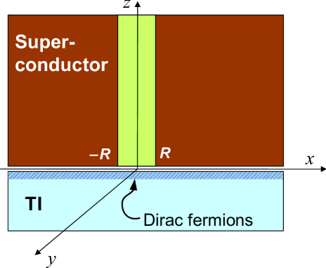
Figure 1: (Color online) Schematic side view of the system studied in this work. On the surface of the topological insulator (TI) there exists a 2D band of surface states which may be described by massless Dirac equation. To induce superconductivity in this 2D metal, a slab of superconducting material (SC) is placed on top of the topological insulator’s surface. A cylindrical cavity of radius $R$ is carved in the superconductor. It serves as a pinning site for the Abrikosov vortex, which is introduced in order to create the Majorana state. The main purpose of the cavity is to remove the unwanted single-particle excitations in the normal core of the vortex. Therefore, a robust Majorana fermion can be localized inside the vortex core created on the surface of the topological insulator by the proximity effect.

II.2 Uniform system

The symbolic Eq. (10) is very general: it is valid for arbitrary $\Delta({\bf R})$ and $\widehat{\cal T}$, as long as the Green’s function remains well-defined. Of course, finding the Green’s function for a non-uniform $\Delta$ may be practically challenging. Fortunately, in the regime of interest the required Green’s function can be constructed from the knowledge of the Green’s function for a homogeneous system. Thus, as a first step, let us study the situation when $\Delta$ and $\widehat{\cal T}$ are uniform over the whole interface, the cavity is absent, and $|\omega|<|\Delta|$. The resultant BdG equation now reads

$$\left(H_{\textrm{eff}}-\omega\right)\Psi_{\textrm{TI}}=0,$$ (11)

where the effective Hamiltonian and its parameters are defined as

$$H_{\textrm{eff}}=\left[i\tilde{v}(\omega)(\mathbf{\sigma}\cdot\mathbf{\nabla}_{\bf r})-\tilde{U}(\omega)\right]\tau_{z}$$ (12)

$$+\tilde{\Delta}^{\prime}(\omega)\tau_{x}+\tilde{\Delta}^{\prime\prime}(\omega)\tau_{y},$$

$$\tilde{v}(\omega)=\frac{v\sqrt{|\Delta|^{2}-\omega^{2}}}{\sqrt{|\Delta|^{2}-\omega^{2}}+\lambda},$$ (13)

$$\tilde{U}(\omega)=\frac{(U+\delta U)\sqrt{|\Delta|^{2}-\omega^{2}}}{\sqrt{|\Delta|^{2}-\omega^{2}}+\lambda},$$ (14)

$$\tilde{\Delta}(\omega)=\tilde{\Delta}^{\prime}(\omega)+i\tilde{\Delta}^{\prime\prime}(\omega)=\frac{\Delta\lambda}{\sqrt{|\Delta|^{2}-\omega^{2}}+\lambda}.$$ (15)

The quantity $\lambda$ has the dimension of energy. It characterizes the transparency of the barrier separating the SC and TI, and can be measured in a tunneling experiment performed at $T>T_{c}$. For our purposes we need a sufficiently thick insulating layer between the superconductor and the TI to guarantee the low transparency of the barrier $(\lambda\ll\varepsilon_{\rm F})$. sau_robustness

The contact with the superconductor shifts the bare Fermi energy $U$ by the amount $\delta U=O(\lambda)$. The details of the derivation can be found in Appendix A.

For uniform $\lambda$ and $\Delta$ we can choose $\Delta$ to be real. Eq. (11) has no solutions with $|\omega|<\Delta_{\rm TI}$, where the proximity-induced gap $\Delta_{\rm TI}<\Delta$ satisfies the equation $\tilde{\Delta}(\Delta_{\rm TI})=\Delta_{\rm TI}$, or, equivalently,

$$\frac{\lambda}{\Delta}=\frac{\Delta_{\rm TI}}{\Delta}\sqrt{\frac{\Delta+\Delta_{\rm TI}}{\Delta-\Delta_{\rm TI}}}.$$ (16)

The gap in the TI is a monotonous function of $\lambda$: $\Delta_{\rm TI}\approx\lambda$ at small $\lambda\ll\Delta$ and approaches $\Delta$ from below at large $\lambda\gg\Delta$.

II.3 The system with the pinned vortex

The system schematically drawn in Fig. 1, however, is not uniform. Due to the cavity and the vortex, both $\Delta$ and $\lambda$ acquire some coordinate dependence. Obviously, $\lambda(r)$ vanishes for $r<R$, where $r=\sqrt{x^{2}+y^{2}}$ is distance to the axis of the cavity. In addition, when the vortex is introduced dG , $\Delta({\bf R})$ can be written as

$$\Delta({\bf R})=|\Delta(r)|e^{i\theta},$$ (17)

where $\theta$ is the polar angle in the $(x,y)$-plane, and $|\Delta(r)|$ is an increasing function of $r$, which approaches the bulk value $|\Delta|$ when $r\rightarrow\infty$. It is finite at $r=R+0$. In such a case, strictly speaking, one has to re-calculate the superconducting Green’s function for a spatially varying $\Delta(r,\theta)$. This might be particularly difficult for $r\lesssim\xi$, where the phase $\theta$ varies quickly on the distances of the order of $\xi$.

However, one can avoid the latter complication if

$$R\gg\xi.$$ (18)

In this limit our formalism can be easily adopted to account for the vortex presence. Ignoring the detailed behavior of $|\Delta(r)|$ when $r\approx R$, we assume that

$$|\Delta(r)|=|\Delta|\vartheta(r-R),$$ (19)

where $\vartheta(r)$ is the Heaviside step-function.

When Eq. (18) holds true, the order parameter phase $\theta$ varies slowly on distances of the order of $\xi$. Thus, it is permissible to insert the non-uniform $\Delta(r,\theta)$, Eq. (17), directly into Eqs. (12)-(15). Since $|\Delta|$ is $r$-dependent, therefore, $\tilde{v}$, $|\tilde{\Delta}|$, and $\tilde{U}$ are non-uniform. Further, we assume that our treatment remains valid, at least qualitatively, in the case $R\gtrsim\xi$.

In our formalism the TI area beneath the cavity ($r<R$) is non-superconducting. It may be viewed as the normal core of “the pancake” vortex. Outside the core (for $r>R$), the absolute value of the order parameter equals to its equilibrium value $|\Delta|$. This approximation is very natural in the case $R>\xi$.

To calculate the eigenenergies of the Hamiltonian Eq. (12) with a vortex, it is standard to exploit the cylindrical symmetry of the problem to separate the variables (for details see Appendix B). If we define the spinor $\Phi$ as

$$\Psi_{\textrm{TI}}=\exp{\left[i\theta(\tau_{z}+\sigma_{z})/2+i\mu\theta\right]}\Phi^{\mu}(r),$$ (20)

$$\Phi^{\mu}=(f_{1}^{\mu},f_{2}^{\mu},f_{3}^{\mu},-f_{4}^{\mu})^{T},$$ (21)

then, its four components satisfy

$$i\tilde{v}\left(\frac{d}{dr}+\frac{\mu+1}{r}\right)f_{2}^{\mu}+|\tilde{\Delta}|f_{3}^{\mu}-(\omega+\tilde{U})f_{1}^{\mu} = 0,$$

$$i\tilde{v}\left(\frac{d}{dr}-\frac{\mu}{r}\right)f_{1}^{\mu}-|\tilde{\Delta}|f_{4}^{\mu}-(\omega+\tilde{U})f_{2}^{\mu} = 0,$$

$$i\tilde{v}\left(\frac{d}{dr}+\frac{\mu}{r}\right)f_{4}^{\mu}+|\tilde{\Delta}|f_{1}^{\mu}-(\omega-\tilde{U})f_{3}^{\mu} = 0,$$ (22)

$$i\tilde{v}\left(\frac{d}{dr}-\frac{\mu-1}{r}\right)f_{3}^{\mu}-|\tilde{\Delta}|f_{2}^{\mu}-(\omega-\tilde{U})f_{4}^{\mu} = 0.$$

This is the most general system of equations describing the sub-gap states near the cavity. Below we study the spectral properties of this system.

III Zero-energy Majorana fermion solution

In this section we will demonstrate that the Hamiltonian $H$ has a zero-energy Majorana fermion solution for arbitrary $R$. First, we will demonstrate this for the case of large $R$, when one can map $H$ on $H_{\rm eff}$. Afterward this result will be generalized for any $R>0$. This section contains some known results (see, e.g, Refs. Jackiw_Nuclear, ; Cheng_Phys.Rev.B_2010, ; bergman, ; ghaemi, ), but these are included here to make the derivation more complete and self-contained.

III.1 Majorana state for large $R$

The system of equations (II.3) can be solved exactly when $\omega=0$, $\mu=0$, and $\delta U(r)=0$. The latter requirement is satisfied only in the presence of the external gate potential which compensates for the Fermi level shift induced by the coupling to the superconductor (see Appendix A). In subsection III.2 it is demonstrated that a non-zero $\delta U(r)$ does not destroy the $\omega=0$ solution.

To find the desired solution we define new functions

$$X_{1}^{\mu}=if_{1}^{\mu}+f_{4}^{\mu}\,,\qquad X_{2}^{\mu}=if_{1}^{\mu}-f_{4}^{\mu}\,,$$

$$Y_{1}^{\mu}=if_{2}^{\mu}+f_{3}^{\mu}\,,\qquad Y_{2}^{\mu}=if_{2}^{\mu}-f_{3}^{\mu}\,.$$ (23)

For these functions the system of Eqs. (II.3) splits into two systems of two equations each:

$$\tilde{v}\frac{dX_{2}^{0}}{dr}+|\tilde{\Delta}|X_{2}^{0}=i\tilde{U}Y_{1}^{0}\,,$$ (24)

$$\tilde{v}\frac{dY_{1}^{0}}{dr}+|\tilde{\Delta}|Y_{1}^{0}+\frac{\tilde{v}}{r}Y_{1}^{0}=i\tilde{U}X_{2}^{0}\,,$$ (25)

and

$$\tilde{v}\frac{dX_{1}^{0}}{dr}-|\tilde{\Delta}|X_{1}^{0}=i\tilde{U}Y_{2}^{0}\,,$$ (26)

$$\tilde{v}\frac{dY_{2}^{0}}{dr}-|\tilde{\Delta}|Y_{2}^{0}+\frac{\tilde{v}}{r}Y_{2}^{0}=i\tilde{U}X_{1}^{0}\,.$$ (27)

An elementary analysis reveals that the system of Eqs. (26)-(27) has no non-zero solution decaying at $r\rightarrow\infty$. Thus, $X_{1}^{0}=Y_{2}^{0}=0$. The non-zero solution of the system of Eqs. (24)-(25) can be written explicitly. Keeping in mind that $\tilde{U}(r)/\tilde{v}(r)=U/v$ is a constant independent of $r$ [see Eqs. (13) and (14)], one derives:

$$\left(\!\begin{array}[]{c}X_{2}^{0}\\ Y_{1}^{0}\\ \end{array}\!\right)\!=2C\!\left(\!\begin{array}[]{c}iJ_{0}(Ur/v)\\ J_{1}(Ur/v)\\ \end{array}\!\right)\exp{\left(-\int_{0}^{r}\frac{dr^{\prime}|\tilde{\Delta}(r^{\prime})|}{\tilde{v}(r^{\prime})}\right)},$$ (28)

where $C$ is a normalizing coefficient, and $J_{0}$, $J_{1}$ are Bessel functions. Thus, the exact solution for $\omega=0$ is

$$\!\!\Psi_{\textrm{M}}({\bf r})\!=\!C\left(\!\!\begin{array}[]{c}\exp(i\theta)J_{0}(Ur/v)\\ -iJ_{1}(Ur/v)\\ J_{1}(Ur/v)\\ i\exp(-i\theta)J_{0}(Ur/v)\\ \end{array}\!\!\right)\!\exp{\left(-\int_{0}^{r}\frac{dr^{\prime}|\tilde{\Delta}(r^{\prime})|}{\tilde{v}(r^{\prime})}\right)}.$$ (29)

If the ratio $|\tilde{\Delta}(r)|/\tilde{v}(r)=\lambda/v$ is a constant independent of $r$ [see Eqs. (13) and (15)] then the spinor $\Psi_{\textrm{M}}$ decays for distances larger than $v/\lambda$, which may be viewed as a characteristic localization length of the zero-energy state.

To prove that the eigenfunction given by Eq. (29) corresponds to the Majorana state, consider the following fermion operator

$$\hat{\Psi}^{\dagger}_{\rm M}=\int d^{2}{\bf r}\left[u^{\rm M}_{\uparrow}({\bf r})\psi^{\dagger}_{\uparrow}({\bf r})+u^{\rm M}_{\downarrow}({\bf r})\psi^{\dagger}_{\downarrow}({\bf r})\right.$$ (30)

$$\left.+v^{\rm M}_{\uparrow}({\bf r})\psi^{\vphantom{\dagger}}_{\uparrow}({\bf r})+v^{\rm M}_{\downarrow}({\bf r})\psi^{\vphantom{\dagger}}_{\downarrow}({\bf r})\right],$$

where $\psi_{\sigma}^{\dagger}({\bf r})$ is the creation operator for an electron with spin $\sigma$ located at point ${\bf r}$. The functions $u^{\rm M}_{\sigma}({\bf r})$, $v^{\rm M}_{\sigma}({\bf r})$ are components of the spinor ${\Psi}_{\rm M}({\bf r})$. The operator $\hat{\Psi}^{\dagger}_{\rm M}$ creates a fermion in the state corresponding to ${\Psi}_{\rm M}({\bf r})$. It is easy to demonstrate, by direct calculation, that $\hat{\Psi}^{\dagger}_{\rm M}=i\hat{\Psi}^{\vphantom{\dagger}}_{\rm M}.$ Therefore, $\Psi_{\rm M}$ corresponds to the Majorana fermion.

III.2 Majorana state for arbitrary $R$ and $U$

We demonstrated above that for large $R$ our system can be mapped to 2D Dirac electrons. In the latter model, when the vortex is present, the zero-energy solution is found Jackiw_Nuclear .

Unfortunately, if $R$ is small, this mapping is inapplicable. What happens to the Majorana state when the cavity is small? Below we will prove that our Hamiltonian has a zero-energy eigenstate for any $R\geq 0$.

We start our reasoning with the observation that $H$ satisfies the following charge-conjugation relation:

$$H=-\tau_{y}\sigma_{y}H^{*}\tau_{y}\sigma_{y}.$$ (31)

Thus, for every eigenstate $\Psi$ of $H$ with a non-zero eigenenergy $\omega\neq 0$, an eigenstate $\tau_{y}\sigma_{y}\Psi^{*}$ with eigenenergy $-\omega$ is present. A spinor with positive eigenenergy corresponds to the creation of a quasiparticle, while the charge-conjugated spinor corresponds to the destruction of this quasiparticle.

Further, it is demonstrated here that for large $R$ the Hamiltonian has the zero-energy solution $\Psi_{\rm M}$. This eigenstate is special for it remains unchanged after a charge-conjugation transformation. This means that the number of eigenenergies lying inside of the even-energy interval $(|\Delta|,-|\Delta|)$ is odd (i.e., all the non-zero eigenstates are paired, while the Majorana state is unpaired). If we start decreasing $R$ this property endures: due to symmetry [see Eq. (31)] the eigenstates can enter or leave our energy interval only in pairs. Thus, for any $R$ the Hamiltonian $H$ has an unpaired $\omega=0$ eigenstate invariant under charge conjugation. However, it is necessary to remember that, when $R<\xi$, the Majorana state cannot be robust due to the CdGM states in the Abrikosov vortex core.

Instead of $R$, one can vary $\delta U$. The above reasoning can be modified to prove that the deviation of $\delta U(r)$ from the $\delta U(r)=0$ value does not destroy the Majorana state.

IV Excited states in the vortex core

In addition to the $\omega=0$ state, it is possible to have $0<|\omega|<|\Delta_{\rm TI}|$ states localized at the vortex core.

IV.1 Analytical calculations

To find the eigenfunctions for these states, it is necessary to solve the system (II.3) for generic $\omega$ and $\mu$. The solution can be simplified significantly for $\tilde{U}=0$. We will now investigate this case. The non-zero $\tilde{U}(r)$ may be accounted with the help of perturbation theory, at least for $|\tilde{U}|\ll\tilde{\Delta}$. According to Eqs. (26) and (27) of Ref. sau_robustness, , the case $|\tilde{U}|>\tilde{\Delta}$ is not favorable for the robustness of the Majorana state and will not be studied here.

When $\tilde{U}=0$ and $r<R$, the system (II.3) decouples into two sets of equations:

$$i{v}\left(\frac{d}{dr}+\frac{\mu+1}{r}\right)f_{2}^{\mu}-\omega f_{1}^{\mu} = 0,$$ (32)

$$i{v}\left(\frac{d}{dr}-\frac{\mu}{r}\right)f_{1}^{\mu}-\omega f_{2}^{\mu} = 0,$$ (33)

and

$$i{v}\left(\frac{d}{dr}+\frac{\mu}{r}\right)f_{4}^{\mu}-\omega f_{3}^{\mu} = 0,$$ (34)

$$i{v}\left(\frac{d}{dr}-\frac{\mu-1}{r}\right)f_{3}^{\mu}-\omega f_{4}^{\mu} = 0.$$ (35)

The solution is

$$f_{1}^{\mu}=iA_{\mu}J_{\mu}(\omega r/{v}),\qquad f_{2}^{\mu}=A_{\mu}J_{\mu+1}(\omega r/{v}),$$

$$f_{3}^{\mu}=iB_{\mu}J_{\mu-1}(\omega r/{v}),\qquad f_{4}^{\mu}=B_{\mu}J_{\mu}(\omega r/{v}),$$ (36)

where $A_{\mu}$ and $B_{\mu}$ are constants.

For $r>R$ the equations are:

$$Y_{2}^{\mu}=\frac{i\tilde{v}}{\omega}\left(\frac{dX_{2}^{\mu}}{dr}+\frac{|\tilde{\Delta}|}{\tilde{v}}X_{2}^{\mu}-\frac{\mu}{r}X_{1}^{\mu}\right),\qquad$$

$$Y_{1}^{\mu}=\frac{i\tilde{v}}{\omega}\left(\frac{dX_{1}^{\mu}}{dr}-\frac{|\tilde{\Delta}|}{\tilde{v}}X_{1}^{\mu}-\frac{\mu}{r}X_{2}^{\mu}\right),\qquad$$ (37)

$$\frac{d^{2}X_{1}^{\mu}}{dr^{2}}+\frac{1}{r}\frac{dX_{1}^{\mu}}{dr}-\left(\frac{1}{[\tilde{\xi}(\omega)]^{2}}+\frac{|\tilde{\Delta}|}{\tilde{v}r}-\frac{\mu^{2}}{r^{2}}\right)X_{1}^{\mu}=0,$$

$$\frac{d^{2}X_{2}^{\mu}}{dr^{2}}+\frac{1}{r}\frac{dX_{2}^{\mu}}{dr}-\left(\frac{1}{[\tilde{\xi}(\omega)]^{2}}-\frac{|\tilde{\Delta}|}{\tilde{v}r}+\frac{\mu^{2}}{r^{2}}\right)X_{1}^{\mu}=0,$$

where the functions $X^{\mu}_{1,2}$ and $Y^{\mu}_{1,2}$ are defined by Eqs. (III.1), and the length $\tilde{\xi}(\omega)$ is given by the formula:

$$\tilde{\xi}(\omega) = \frac{\tilde{v}(\omega)}{\sqrt{|\tilde{\Delta}(\omega)|^{2}-\omega^{2}}}.$$ (38)

The above equations may be solved AbrSteg in terms of the Whittaker functions $W_{\alpha,\beta}(z)$:

$$X^{\mu}_{1,2}=\frac{C_{1,2}}{\sqrt{r}}W_{\alpha_{1,2},\mu}\left(2r/\tilde{\xi}(\omega)\right),$$ (39)

$$\alpha_{1,2}=\mp\frac{|\tilde{\Delta}|}{2\sqrt{|\tilde{\Delta}|^{2}-\omega^{2}}}.$$ (40)

Using Eq. (16) one can show that for subgap states ($|\omega|<\Delta_{\rm TI}$) the expression under the square root in Eqs. (38) and (40) is positive, therefore, $\tilde{\xi}(\omega)$ and $\alpha_{1,2}$ are real. Equation (39) implies that $\tilde{\xi}(\omega)$ is the energy-dependent localization length for the subgap states.

Matching the solutions at $r=R$ we derive the equation for the subgap eigenenergies:

$$\left(\frac{W^{\prime}_{\alpha_{1},\mu}}{\tilde{\xi}W_{\alpha_{1},\mu}}+\frac{W^{\prime}_{\alpha_{2},\mu}}{\tilde{\xi}W_{\alpha_{2},\mu}}-\frac{\mu+1}{R}+\frac{\omega J_{\mu+1}}{\tilde{v}J_{\mu}}\right)$$ (41)

$$\times\left(\frac{W^{\prime}_{\alpha_{1},\mu}}{\tilde{\xi}W_{\alpha_{1},\mu}}+\frac{W^{\prime}_{\alpha_{2},\mu}}{\tilde{\xi}W_{\alpha_{2},\mu}}+\frac{\mu-1}{R}-{\omega J_{\mu-1}\over{\tilde{v}J_{\mu}}}\right)$$

$$=\left(\frac{W^{\prime}_{\alpha_{1},\mu}}{\tilde{\xi}W_{\alpha_{1},\mu}}-\frac{W^{\prime}_{\alpha_{2},\mu}}{\tilde{\xi}W_{\alpha_{2},\mu}}-\frac{\tilde{\Delta}}{\tilde{v}}\right)^{2}.$$

In this equation all functions $W_{\alpha,\beta}(z)$ and $W^{\prime}_{\alpha,\beta}(z)$ must be evaluated at $z=2R/\tilde{\xi}(\omega)$, and all Bessel functions must be evaluated at $\omega R/v$. We analyzed Eq. (41) numerically.

IV.2 Majorana fermion robustness

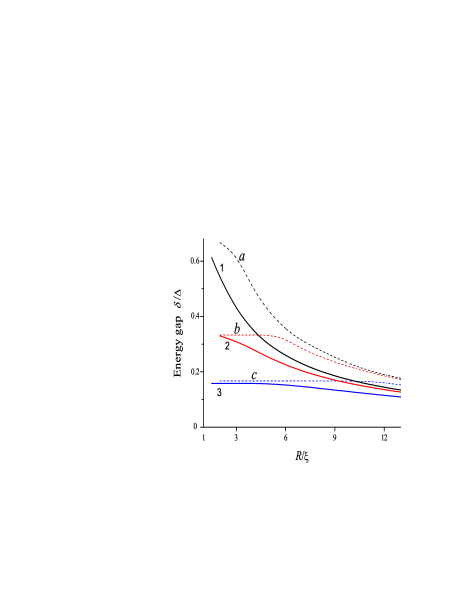
Figure 2: (Color online) The energy gap $\delta$ between the ground state and excited states as a function of the cavity radius $R$, for different transparencies $\lambda$ of the barrier. The solid curves 1, 2, and 3 correspond to the states with $n=0,\,\mu=1$, and the dashed curves a, b, c correspond to the states with $n=1,\,\mu=0$. As we go from top to bottom, the transparency $\lambda$ decreases: curves 1 and a (black) are drawn for $\lambda/\Delta=2$; curves 2 and b (red) are drawn for $\lambda/\Delta=0.5$; curves 3 and c (blue) are drawn for $\lambda/\Delta=0.1$.

The excited quantum states of our system can be classified using two quantum numbers: the radial number $n$ and the orbital number $\mu$. The Majorana state obtained above corresponds to the $n=0,\,\mu=0$ state. The results of the numerical solution of Eq. (41) for different values of ($n,\,\mu$) are shown in Fig. 2. Here the reduced gaps $\delta/\Delta$ between the ground state and excited states with ($n=0,\,\mu=1$) and ($n=1,\,\mu=0$) are plotted for different transparencies $\lambda$ as a function of the cavity radius $R$. The solution of Eq. (41) confirms an intuitively transparent conclusion: that the first excited state is either the ($n=0,\,\mu=1$) state, or the ($n=1,\,\mu=0$) state. Note, that, to calculate $\delta$ in the case ($n=1,\,\mu=0$), we use the asymptotics of the Whittaker functions $W_{\alpha_{1,2},0}(z)$ valid at $|z|\gg 1$. This negatively affects the accuracy of our calculations at small $R$. We believe, however, that this substitution does not distort the qualitative features of the solution.

As it is seen from Fig. 2, the state ($n=0,\,\mu=1$) lies lower than the state ($n=1,\,\mu=0$). Thus, the gap between the ground state and the excited state ($n=0,\,\mu=1$) characterizes the robustness of the Majorana fermion in our system. The gap value increases when $\lambda$ increases. If $\lambda\gtrsim\Delta$, the energy gap $\delta(R)$ practically saturates and further growth of the barrier transparency does not significantly improve the robustness. Experimentally, the regime $\lambda\sim\Delta$ corresponds to a barrier with low transparency sau_robustness , since $\lambda$ is much smaller than the Fermi energy.

At a given $\lambda$, the curve $\delta(R)$ is a decreasing function of $R$, approaching a maximum value

$$\delta_{\textrm{max}}=\tilde{\Delta}(0)=\frac{\Delta\lambda}{(\Delta+\lambda)}{\rm\ at\ }R\sim\xi.$$ (42)

The main conclusion that follows from the results shown in Fig. 2 is that the energy gap between the Majorana state and the first excited state may be of the order of $\Delta$ ($\delta/\Delta=0.5$–$0.6$ or even higher) if $\lambda/\Delta\gtrsim 1$–$3$ and $R/\xi=2$–$3$. Therefore, a suitable choice of $R$ and $\lambda$ allows one to realize the robust Majorana state.

IV.3 Physical and intuitive explanation of the Majorana state robustness

Above we demonstrated that in our system a robust Majorana state exists. Our results agree with previous numerical calculations sau_robustness . However, it is desirable to have a simple non-technical physical argument explaining these results. To this end, now consider the “pancake” core. It can be approximately described as a circle of radius $R$, where the superconducting gap is zero. Let us now evaluate the number $N^{\rm core}_{\rm TI}$ of the single-electron subgap states:

$$N^{\rm core}_{\rm TI}\sim\pi R^{2}\!\!\int_{0}^{\Delta_{\rm TI}}\!\!\!\!\nu_{\rm TI}(\epsilon)\;d\epsilon\;\sim\;\frac{\Delta^{2}_{\rm TI}R^{2}}{v^{2}}.$$ (43)

Here $\nu_{\rm TI}(\epsilon)\sim\epsilon/v^{2}$ is the density of states for the TI. The average energy interval between these states is

$$\delta_{\rm TI}\;\sim\;\Delta_{\rm TI}/N^{\rm core}_{\rm TI}\;\sim\;v^{2}/(R^{2}\Delta_{\rm TI}).$$ (44)

For $R\sim\xi$ and $\Delta_{\rm TI}\sim\Delta$, one has $N^{\rm core}_{\rm TI}\sim 1$ and $\delta_{\rm TI}\sim\Delta$. The last estimate is equivalent to the statement of the Majorana fermion robustness.

If, instead of TI, we now consider a 2D superconductor with parabolic dispersion, we then obtain:

$$N_{\rm m}^{\rm core}\;\sim\;\pi R^{2}\Delta\nu_{\rm m}(\varepsilon_{\rm F})\;\sim\;\left(\frac{\varepsilon_{\rm F}}{\Delta}\right)\!\frac{R^{2}}{{\xi}^{2}}.$$ (45)

Here $\nu_{\rm m}(\varepsilon)$ is the density of states for a 2D metal [$\nu_{\rm m}(\varepsilon)=4m$]. When $R\sim\xi$, the number $N_{\rm m}^{\rm core}$ is much greater than unity. Further, the energy difference between the CdGM energy levels is of the order of $(\Delta^{2}/\varepsilon_{\rm F})(\xi^{2}/R^{2})$. For $R\sim\xi$ we recover Eq. (1).

The estimate of the previous paragraphs demonstrates that the source of robustness of the Majorana fermion in TI is the vanishing density of states at the Dirac point. If we were to apply a bias shifting the Fermi level away from the Dirac point, at a bias value $U$ substantially exceeding $\tilde{\Delta}$, we recover Eq. (1). Thus, $U=0$ is a favorable condition for the Majorana state robustness.

V Discussion and conclusion

We demonstrated that in the proposed system a robust Majorana state may exist. A possible way to detect its presence is to perform the following tunneling experiment: insert an STM tip into the cavity and measure the electron current flowing through the TI surface. In such a setup the Majorana state manifests itself as a zero-bias anomaly: a peak of the differential conductance located at $eV=0$. Unlike the zero-bias anomaly observed for an Abrikosov vortex in a BCS superconductor ZBA1 ; ZBA2 , in the case of the robust Majorana state, the zero-bias anomaly is accompanied by several discrete subgap peaks which correspond to the excited states bound in the vortex core.

We would like to compare our proposal with the system discussed in Ref. sau_robustness, . It is clear that in our system the Majorana fermion is pinned to the cavity. The advantage of the setup in Ref. sau_robustness, is that it allows one to shift the Majorana fermion along a straight channel over the distance $L\sim\xi$. However, the robustness of the Majorana state decreases when one tries to increase the distance $L$ above $\xi$: the gap separating the Majorana fermion and the lowest excited state can be estimated as $\delta\sim v/L$ for $L>\tilde{\xi}$. Moreover, the complexity of their sau_robustness system is an additional limitation.

To conclude, we propose a SC-TI setup in which a robust Majorana state may be realized inside the core of the pinned vortex. The robustness was justified with the help of both analytical and physically intuitive arguments. An experimental detection of this state is also discussed.

Appendix A Derivation of the effective Hamiltonian for proximity-induced superconductivity

In this Appendix we briefly present a derivation of the effective BdG equation at the TI surface. Here we refine the reasoning of Ref. sau_robustness, ; sau_preprint, .

The system in question consists of a superconducting slab, described by the BCS Hamiltonian $H_{\rm SC}$, and a topological insulator with Hamiltonian $H_{\rm TI}$. These two are separated by a flat interface. Tunneling across this interface is described by the tunneling Hamiltonian: $\widehat{\cal T}+\widehat{\cal T}^{\dagger}$.

As the TI has the bulk gap, its low-energy states are located at the surface. At low energy these 2D states can be approximately described by the Weyl-Dirac Hamiltonian whose apex is located at the ${\bf M}$ point at the boundary of the Brillouin zone of the TI.

Due to conservation of the spin and the quasi-momentum parallel to the flat interface, the tunneling Hamiltonian couples a single-electron state $\left|\phi^{\rm TI}_{{\bf k}\sigma}\right>$ inside the TI with a normal-metal state $\left|\chi^{\rm m}_{{\bf M+k},k_{z},\sigma}\right>$ inside the superconductor. Here $\sigma$ is the spin index, ${\bf k}$ is the momentum’s components parallel to the barrier measured from ${\bf M}$, and ${k}_{z}$ is the absolute value of the transverse momentum (since scattering at the interface couples SC states with $k_{z}$ and $-k_{z}$, the state $\left|\chi^{\rm m}_{{\bf M+k},k_{z},\sigma}\right>$ is a boundary-condition-compatible linear combination of both $k_{z}$ and $-k_{z}$ states). The superscript ‘m’ stands for ‘metal’. Let us denote the corresponding matrix element by ${\cal T}({\bf k},k_{z})$. It is assumed to be spin independent.

Invariance of the tunneling Hamiltonian with respect to the spatial inversion ${\bf r}\rightarrow-{\bf r}$ implies that the same matrix element couples the states $\left|\phi^{\rm TI}_{-{\bf k}\sigma}\right>$ and $\left|\chi^{\rm m}_{{\bf-M-k},k_{z},\sigma}\right>$. Indeed, the quasi-momentum ${\bf M-k}$ of the TI state is equal to the momentum ${\bf-M-k}$ of the state inside the superconductor, modulo the TI’s reciprocal lattice vector $2{\bf M}$. Thus, the anomalous term of $H_{\rm SC}$, which mixes $\left|\chi^{\rm m}_{{\bf-M-k},k_{z},\sigma}\right>$ and $\left|\chi^{\rm m}_{{\bf M+k},k_{z},\sigma}\right>$, induces a coupling between $\left|\phi^{\rm TI}_{{\bf k}\sigma}\right>$ and $\left|\phi^{\rm TI}_{-{\bf k}\sigma}\right>$ in $H_{\rm eff}$.

In addition, recall that for a tunneling matrix element ${\cal T}$ between certain electronic states there is a tunneling matrix element $-{\cal T}$ between corresponding charge-conjugated states. This implies that the operator $\widehat{\cal T}$ in the Nambu representation Eq. (8) is proportional to $\tau_{z}$, see Eq. (7).

The single-quasiparticle states are given by the following BdG equations

$$\left(H_{\textrm{TI}}-\omega\right)\Psi_{\textrm{TI}}+{\cal{T}}^{\dagger}\Psi_{\textrm{SC}} = 0,$$

$$\left(H_{\textrm{SC}}-\omega\right)\Psi_{\textrm{SC}}+{\cal{T}}\Psi_{\textrm{TI}} = 0.$$ (46)

The four-component spinor $\Psi_{\textrm{SC}}$ ($\Psi_{\textrm{TI}}$) describes a quasiparticle inside the SC (TI).

Solving the second of the Eqs. (A) for the wave-function $\Psi_{\textrm{SC}}$ and substituting the resultant expression in the first one, we derive the effective BdG equation on the TI surface

$$\left[H_{\textrm{TI}}+\Sigma(\mathbf{k},\omega)-\omega\right]\Psi_{\textrm{TI}}=0,$$ (47)

where the self-energy $\Sigma$ on the TI surface reads

$$\Sigma(\mathbf{k},\omega)=-\frac{1}{L_{z}}\sum_{k_{z}}\left|{\cal{T}}(\mathbf{k},k_{z})\right|^{2}\tau_{z}\>G_{\textrm{SC}}(\mathbf{k},k_{z},\omega)\>\tau_{z}.$$ (48)

The Green’s function for the superconductor $G_{\textrm{SC}}=\left(H_{\textrm{SC}}-\omega\right)^{-1}$ can be derived with the help of Eq. (6):

$$G_{\textrm{SC}}(\mathbf{k},k_{z},\omega)=\left[\epsilon(\mathbf{k},k_{z})\tau_{z}+\Delta\tau_{x}-\omega\tau_{0}\right]^{-1},$$ (49)

where $\epsilon(\mathbf{k},k_{z})=\left(k^{2}+k_{z}^{2}\right)/2m-\varepsilon_{F}$. Substituting Eq. (49) in Eq. (48), one obtains

$$\Sigma(\mathbf{k},\omega)=\int\frac{dk_{z}}{2\pi}\frac{\Delta\tau_{x}-\omega\tau_{0}-\epsilon\tau_{z}}{\epsilon^{2}+|\Delta|^{2}-\omega^{2}}\left|{\cal{T}}({{\bf k},k_{z}})\right|^{2}.$$ (50)

Here $\tau_{0}$ is the unit matrix. The tunneling matrix element ${\cal{T}}({{\bf k},k_{z}})$ is assumed to vary slowly as a function of $k_{z}$. Then, transforming the $k_{z}$ integral to an energy one, we derive

$$\Sigma(\mathbf{k},\omega)\approx\lambda(\mathbf{k})\frac{\Delta\tau_{x}-\omega\tau_{0}}{\sqrt{|\Delta|^{2}-\omega^{2}}}-\delta U\tau_{z},$$ (51)

where $\lambda(\mathbf{k})=(\pi/2)\nu(\varepsilon_{F},\mathbf{k})\left|{\cal{T}}({{\bf k},k_{z}})\right|^{2}$ characterizes the transparency of the interface. The quantity $\nu(\varepsilon,\mathbf{k})$ quantifies the DOS at a given energy and parallel momentum in the normal state of the SC. It is equal to

$$\nu(\varepsilon,\mathbf{k})=\int\frac{dk_{z}}{2\pi}\delta\left[\varepsilon-\epsilon(\mathbf{k},k_{z})\right].$$ (52)

In what follows we are interested in states close to the Dirac cone $\mathbf{k}=\mathbf{M}$ and ignore the k-dependence of $\lambda$, assuming that $\lambda({\bf k})\approx\lambda({\bf M})$.

The correction to the TI Fermi energy due to tunneling is equal to

$$\delta U=\int\frac{dk_{z}}{2\pi}\frac{\epsilon\left|{\cal{T}}({{\bf k},k_{z}})\right|^{2}}{\epsilon^{2}+|\Delta|^{2}-\omega^{2}}\approx\lambda(\mathbf{M})\int^{E_{\rm h}}_{-E_{\rm e}}\frac{d\epsilon}{\epsilon}$$ (53)

$$\approx\lambda({\bf M})\ln\frac{E_{\rm h}}{E_{\rm e}}=O(\lambda),$$

where $E_{\rm h}$ ($E_{\rm e}$) is the largest hole (electron) energy relative to the Fermi level, and the integral over $1/\epsilon$ is taken using the Cauchy principle value. This term is, in general, non-zero. It was discarded in Ref. sau_robustness, , presumably, because it can be absorbed into the renormalized Fermi energy. However, if $\lambda$ depends on the position ${\bf r}$ (which is the case for both our system as well as the system of Ref. sau_robustness, ), then $\delta U$ becomes spatially inhomogeneous as well. Under such circumstances, $\delta U({\bf r})$ cannot be absorbed into the Fermi energy, and has to be treated separately. It should be possible, however, to compensate $\delta U$ by an external gate potential.

Finally, using $H_{\textrm{TI}}$ from Eq. (5) and $\Sigma$ from Eq. (51), we rewrite Eq. (47) in the explicit form sau_robustness

$$\left(H_{\textrm{eff}}-\omega\right)\Psi_{\textrm{TI}}=0,$$ (54)

$$H_{\textrm{eff}}=\left[i\tilde{v}(\omega)(\mathbf{\sigma}\cdot\mathbf{\nabla}_{\bf r})-\tilde{U}(\omega)\right]\tau_{z}+\tilde{\Delta}(\omega)\tau_{x},$$ (55)

$$\tilde{v}(\omega)=\frac{v\sqrt{|\Delta|^{2}-\omega^{2}}}{\sqrt{|\Delta|^{2}-\omega^{2}}+\lambda},$$ (56)

$$\tilde{U}(\omega)=\frac{(U+\delta U)\sqrt{|\Delta|^{2}-\omega^{2}}}{\sqrt{|\Delta|^{2}-\omega^{2}}+\lambda},$$ (57)

$$\tilde{\Delta}(\omega)=\frac{\Delta\lambda}{\sqrt{|\Delta|^{2}-\omega^{2}}+\lambda}.$$ (58)

Appendix B Bogolyubov-de Gennes equations for the radial motion

In this Appendix we will exploit the cylindrical symmetry of the problem, to separate angular and radial variables, and to derive the equations for the radial part of the wave function. The effective Hamiltonian with a single vortex is equal to

$$H_{\textrm{eff}} = i\tilde{v}(r)\exp{\left(i\theta\sigma_{z}\right)}\left(\sigma_{x}\partial_{r}+\frac{1}{r}\sigma_{y}\partial_{\theta}\right)\tau_{z}$$

$$+ |\tilde{\Delta}(r)|\exp{\left(i\frac{\theta}{2}\tau_{z}\right)}\tau_{x}\exp{\left(\!-i\frac{\theta}{2}\tau_{z}\right)}-\tilde{U}(r)\tau_{z}\,.$$

The first term here is the Weyl-Dirac Hamiltonian in polar coordinates. The second term corresponds to the anomalous term in the presence of a vortex.

Equation (B) suggests that it is useful to define a new spinor $\Psi$

$$\Psi_{\textrm{TI}}=\exp{\left[i\theta(\tau_{z}+\sigma_{z})/2\right]}\Psi.$$ (60)

Accordingly, the effective Hamiltonian is transformed as

$$H^{\prime}_{\textrm{eff}}=\exp{\left[-i\theta(\tau_{z}+\sigma_{z})/2\right]}H_{\textrm{eff}}\exp{\left[i\theta(\tau_{z}+\sigma_{z})/2\right]}.\qquad$$ (61)

The equation for $\Psi$ now reads

$$\Big{\{}i\tilde{v}\left[\sigma_{x}\partial_{r}+\frac{1}{r}\sigma_{y}\partial_{\theta}+\frac{i}{2r}\sigma_{y}(\tau_{z}+\sigma_{z})\right]\tau_{z}$$

$$+|\tilde{\Delta}|\tau_{x}-\tilde{U}\tau_{z}-{\omega}\Big{\}}\Psi=0\,.$$ (62)

We look for a solution of Eq. (B) in the form $\Psi=e^{i\mu\theta}\Phi^{\mu}$, where $\mu=0,\pm 1,\pm 2,...$ is the angular momentum. The values of $\mu$ are integers (not half-integers) to ensure single-valuedness of $\Psi_{\rm TI}$. It is straightforward to show now that the components of the spinor $\Phi^{\mu}=(f_{1}^{\mu},f_{2}^{\mu},f_{3}^{\mu},-f_{4}^{\mu})^{T}$ satisfy Eq. (II.3).

References

- (1)
- (2) V. Emery and S. Kivelson, Phys. Rev. B46, 10812 (1992)
- (3) A.V. Rozhkov, Int. J. Mod. Phys. B 12, 3457 (1998).
- (4) G. Zarand and J. von Delft, Phys. Rev. B61, 6918 (2000).
- (5) B.S. Shastry and D. Sen, Phys. Rev. B55, 2988 (1997).
- (6) C. Nayak, S.H. Simon, A. Stern, M. Freedman, and S. Das Sarma, Rev. Mod. Phys. 80, 1083 (2008).
- (7) S.B. Chung and S.C. Zhang, Phys. Rev. Lett. 103, 235301 (2009).
- (8) G.E. Volovik, JETP Lett. 90, 398 (2009).
- (9) C. Benjamin and J.K. Pachos, Phys. Rev. B81, 085101 (2010).
- (10) J. Alicea, Phys. Rev. B81, 125318 (2010).
- (11) Y.E. Kraus, A. Auerbach, H.A. Fertig, and S.H. Simon, Phys. Rev. Lett. 101, 267002 (2008).
- (12) Y.E. Kraus, A. Auerbach, H.A. Fertig, and S.H. Simon, Phys. Rev. B79, 134515 (2009).
- (13) S. Fujimoto, Phys. Rev. B77, 220501 (2008).
- (14) M. Sato and S. Fujimoto, Phys. Rev. B79, 094504 (2009).
- (15) L. Fu and C.L. Kane, Phys. Rev. Lett. 100, 096407 (2008).
- (16) J.D. Sau, R.M. Lutchyn, S. Tewari, and S. Das Sarma, Phys. Rev. B82, 094522 (2010).
- (17) M. Sato, Y. Takahashi, and S. Fujimoto, Phys. Rev. Lett. 103, 020401 (2009); Phys. Rev. B 82, 134521 (2010); M. Sato and S. Fujimoto, Phys. Rev. Lett. 105, 217001 (2010).
- (18) D.A. Ivanov, Phys. Rev. Lett. 86, 268 (2001).
- (19) C. Caroli, P.G. de Gennes, and J. Matricon, Phys. Lett. 9, 307 (1964); R.G. Mints and A.L. Rakhmanov, Solid State Commun. 16, 747 (1975).
- (20) A. R. Akhmerov, Phys. Rev. B 82, 020509(R) (2010).
- (21) M. Cheng, R.M. Lutchyn, V. Galitski, and S. Das Sarma, Phys. Rev. B82, 094504 (2010).
- (22) P.G. de Gennes, Superconductivity of Metals and Alloys (Westview Press, 1999).
- (23) R. Jackiw and P. Rossi, Nucl. Phys. B 190, 681 (1981).
- (24) D.L. Bergman and K. Le Hur, Phys. Rev. B 79, 184520 (2009)
- (25) P. Ghaemi and F. Wilczek, arXiv:0709.2626v1 (unpublished).
- (26) M. Abramowitz and I.A. Stegun, Handbook of mathematical functions (NBS, 1972).
- (27) H.F. Hess, R.B. Robinson, R.C. Dynes, J.M. Valles, and J.V. Waszczak, Phys. Rev. Lett. 62, 214 (1989).
- (28) J.D. Shore, M. Huang, A.T. Dorsey, and J.P. Sethna, Phys. Rev. Lett. 62, 3089 (1989).
- (29) J.D. Sau, R.M. Lutchyn, S. Tewari, S. Das Sarma, arXiv:0912.4508v3 (unpublished).