Profiles of Dark Matter Velocity Anisotropy in Simulated Clusters

Abstract

We report statistical results for dark matter (DM) velocity anisotropy, $\beta$, from a sample of some 6000 cluster-size halos (at redshift zero) identified in a $\Lambda$CDM hydrodynamical adaptive mesh refinement simulation performed with the Enzo code. These include profiles of $\beta$ in clusters with different masses, relaxation states, and at several redshifts, modeled both as spherical and triaxial DM configurations. Specifically, although we find a large scatter in the DM velocity anisotropy profiles of different halos (across elliptical shells extending to at least $\sim 1.5r_{\rm vir}$), universal patterns are found when these are averaged over halo mass, redshift, and relaxation stage. These are characterized by a very small velocity anisotropy at the halo center, increasing outward to $\sim 0.27$ and leveling off at $\sim 0.2r_{\rm vir}$. Indirect measurements of the DM velocity anisotropy fall on the upper end of the theoretically expected range. Though measured indirectly, the estimations are derived by using two different surrogate measurements - X-ray and galaxy dynamics. Current estimates of the DM velocity anisotropy are based on very small cluster sample. Increasing this sample will allow testing theoretical predictions, including the speculation that the decay of DM particles results in a large velocity boost. We also find, in accord with previous works, that halos are triaxial and likely to be more prolate when unrelaxed, whereas relaxed halos are more likely to be oblate. Our analysis does not indicate that there is significant correlation (found in some previous studies) between the radial density slope, $\gamma$, and $\beta$ at large radii, $0.3\;r_{\rm vir}<r<r_{\rm vir}$.

1. Introduction

Dark matter (DM), the main mass constituent of galaxy clusters, dominates the dynamics of intracluster (IC) gas and member galaxies. The DM mass density profile was until recently the only cluster property that could be inferred from simulations and tested against observational data. The DM velocity anisotropy profile also holds important information, since it depends on both the DM particle features, such as its collisionless nature (e.g. Host et al. 2009) and decaying time (Peter, Moody, & Kamionkowski 2010), and the wide variety of dynamical collapse processes (Wang & White 2009). In addition, halo mass dynamical estimators, such as Jeans (Binney & Tremaine 2008) and the caustics (Diaferio & Geller 97; Diaferio 99), that use galaxy information, depend on the galaxy velocity anisotropy. Since large hydrodynamical cosmological simulations that include galaxies are not found, one can use the DM velocity anisotropy, since both (DM and galaxies) are considered to be collisionless, and therefore should have similar dynamical properties. That said, measured galaxy velocity anisotropy profiles (e.g. Benatov et al. 2006; Lemze et al. 2009) maybe somewhat different than the ones estimated for DM using simulations. Some effort is now devoted to determine also the DM velocity anisotropy either by using the gas temperature as a tracer of the DM velocity anisotropy, a method which is applicable at intermediate radii (Host et al. 2009), or by examining galaxy velocities, as has recently been demonstrated in the analysis of A1689 measurements (Lemze et al. 2011). It is in fact our plan to apply the latter procedure to additional relaxed X-ray clusters in the CLASH program (Postman et al. 2012).

N-body simulations (for various cosmological models) suggest a nearly universal velocity anisotropy profile (Cole & Lacey 1996; Carlberg et al. 1997; Colin, Klypin, & Kravtsov 2000; Diemand, Moore, & Stadel 2004; Rasia et al. 2004; Wojtak et al. 2005), similar to the universal DM density profile deduced from simulations (Navarro, Frenk, & White 1997, hereafter NFW; Moore et al. 1998)and various observations (X-ray: e.g. Pointecouteau, Arnaud, & Pratt 2005; Arnaud, Pointecouteau, & Pratt 2005; Vikhlinin et al. 2006; Schmidt & Allen 2007; galaxy velocity distributions: Diaferio, Geller, & Rines 2005; SZ measurements: Atrio-Barandela et al. 2008; strong and weak lensing measurements: Broadhurst et al. 2005a, hereafter B05a; Broadhurst et al. 2005b, hereafter B05b; Limousin et al. 2007; Medezinski et al. 2007; Lemze et al. 2008, hereafter L08; Broadhurst et al. 2008; Zitrin et al. 2009, 2010, 2011; Umetsu et al. 2010). If both the density and velocity anisotropy profiles are indeed universal, they must be correlated. Hansen & Moore (2006, hereafter HM06), who used N-body simulation, have recently argued for a universal relation between the DM radial density slope $\gamma(r)$ and the velocity anisotropy $\beta(r)$ for structures in virial equilibrium. Their deduced relation was claimed to hold for various systems, including disk galaxy mergers, simulated halos undergoing spherical collapse, and CDM halos both with and without cooling.

However, while an analysis of 6 high-resolution simulated galactic halos from the Aquarius project, carried out by Navarro et al. (2010), exhibited a reasonably good fit to the HM06 relation in the inner regions, large deviations were reported outside $r_{-2}$, the radius at which the profile slope reaches $-2$. Analogous results were obtained in a study conducted by Tissera et al. (2010), in which they resimulated 6 (Aquarius) galactic halos, constructed so as to include metal-dependent cooling, star formation, and supernova feedback. In 3 of the halos a rather good match to the HM06 relation was found at small radii, $2\,\,kpc\cdot h^{-1}<r<r_{-2}$, but no corresponding match was found in the other 3 halos. No evidence is seen for the HM06 relation at large radii, $r>r_{-2}$, in any of the six halos. Ludlow et al. 2011, who used cosmological N-body simulations, analyzed relaxed halos with mass above $\sim 3.4\times 10^{12}$ h^-1 M_⊙ and fitted an Einasto (1965) profile to the mass density profile. They found a good agreement to the HM06 relation in the inner regions, i.e. $r<r_{-2}$, and for profiles with high Einasto logarithmic slope values, $\gtrsim 0.2$, a better agreement with the HM06 relation achieved even for larger radii. Such a relation between the DM density and velocity anisotropy is of interest, since if it exists in relaxed systems, as claimed in previous works (e.g. Hansen & Stadel 2006; Hansen 2009), this can be an indicator for the system relaxation level. In addition, since DM velocity anisotropy is not easily measurable, whereas the density profile can be determined in several different ways based on different sets of measurements, we can use the $\gamma(r)$ - $\beta(r)$ relation to infer the DM velocity anisotropy from the density profile.

We report the results of an analysis of a large number of cluster-size halos drawn from an Adaptive Mesh Refinement (AMR) cosmological simulation (for details see § 2). The large number of halos at different redshifts allows us to address the dependence of the DM velocity anisotropy profile on redshift, halo mass, degree of relaxation, modeled both as spherical and triaxial DM configurations, and to address also the $\gamma$-$\beta$ relation. The outline of the paper is as follows. In § 2 we describe the simulation dataset, and in § 3 we describe how we infer the radial profiles of the density and velocity anisotropy in spherical and elliptical shells. In § 4 we specify our criteria for relaxed halos, and in § 5 we present halos ellipticities at different relaxation levels, the $\beta$ profiles for different halo mass, redshift, and relaxation stages, and the deduced $\gamma-\beta$ relation. Then in § 6 we discuss our findings, and we conclude in § 7.

2. The simulation

Clusters of galaxies were found using the HOP halo-finding algorithm (Eisenstein & Hut 1998) from a cosmological AMR simulation performed with the hydrodynamical ENZO code developed by Bryan & Norman (1997; see also Norman & Bryan 1999; Norman et al. 2007), assuming a spatially flat $\Lambda$CDM model with the parameters $\Omega_{m}=0.3$, $\Omega_{b}=0.04$, $\Omega_{CDM}=0.26$, $\Omega_{\Lambda}=0.7$, $h=0.7$ (in units of 100 km/s/Mpc), and $\sigma_{8}=0.9$. We also used an Eisenstein & Hu (1999) power spectrum with a spectral index of $n=1$. The hydrodynamics in the AMR simulation used an ideal gas equation of state (i.e., neither radiative heating, cooling, star formation or feedback were included), with a box size of 512 h^-1 Mpc comoving on a side with $512^{3}$ DM particles, and DM mass resolution of about $10^{11}$ h${}_{0.7}^{-1}$ M_⊙. The root grid contained $512^{3}$ grid cells, and the grid was refined by a factor of two, up to seven levels, providing a maximum possible spatial resolution of $7.8$ $(1+z)^{-1}$ h^-1 kpc (this resolution is dependent on the criteria for refinement of the adaptive mesh, and we used the actual resolution when analyzing the halos). For more details on the simulation setup and analysis, see Hallman et al. (2007), in particular Section 2.2.

To find the desired halo DM properties we extracted particle positions and velocities from the raw data. Particles within a cube with comoving side of 16 h^-1 Mpc were extracted. This ensured that both the halo and a sufficiently large surrounding region was available for examination. We had $6019$, $1391$, and $69$ halos with $M_{\rm vir}\geqslant 10^{14}$ h${}_{0.7}^{-1}$ M_⊙ at $z=0$, $z=1$, and $z=2$, respectively.

3. Radial profiles

3.1. Measuring halos shape

Radial profiles were extracted in both spherical and triaxial shells. The mass distribution is described in terms of the axial ratios of the density surface contours. Assuming that the density distribution is stratified in similar ellipsoids, it is possible to determine the axial ratios without knowledge of the radial density distribution (Dubinski & Carlberg 1991, but see also other works e.g. Katz 1991; Warren et al. 1992; Jing et al. 1995; Jing & Suto 2002; Allgood et al. 2006, and references therein). The mass density in a triaxial configuration, $\rho\equiv\rho(r_{\rm e})$, is specified in terms of the elliptical distance in the eigenvector coordinate system of the halo particles, $r_{\rm e}$,

$$r_{\rm e}=\left(x^{2}+\frac{y^{2}}{q^{2}}+\frac{z^{2}}{s^{2}}\right)^{1/2}\,$$ (1)

where $q$ and $s$ are the normalized axial ratios with $s\leqslant q\leqslant 1$.

These ratios can be derived from the tensor

$$M_{\rm ij}=\sum\frac{x_{\rm i}x_{\rm j}}{r_{\rm e}^{2}}\,$$ (2)

through

$$q=\left(\frac{M_{\rm yy}}{M_{\rm xx}}\right)^{1/2}\;\;\;{\rm and}\;\;\;s=\left(\frac{M_{\rm zz}}{M_{\rm xx}}\right)^{1/2}\,$$ (3)

where the sum is over all the particles, and $M_{\rm xx}$, $M_{\rm yy}$, and $M_{\rm zz}$ are the principal components of the diagonalized tensor, with $M_{\rm zz}\leqslant M_{\rm yy}\leqslant M_{\rm xx}$. An advantage of this scheme is the equal weighting given to each particle irrespective of its radial position (see Zemp et al. 2011). The large number of particles in each halo allows accurate determination of the axial ratios. In practice, the value of $r_{\rm e}$ in $M_{\rm ij}$ is not known in advance, due to its dependence on $q$ and $s$ through eq. 1. The axial ratios are therefore determined iteratively. $M_{\rm ij}$ is initially calculated assuming that the contours are spherical, so that $q=s=1$. Particle positions are first rotated into the diagonalized frame of $M_{\rm ij}$, where only particles inside of the ellipse volume were taken (a sphere, in the first iteration). The values of $q$ and $s$ are determined from $M_{\rm ij}$ and then used to recalculate $r_{\rm e}$ in this new frame and fed back into the $M_{\rm ij}$ relation to determine iterated values of $q$ and $s$. When the input values match the output values within a certain tolerance, convergence to the true axial ratios is achieved.

In each iteration new values for $q$ and $s$ are determined, so the halo volume is deformed. We kept the magnitude of the semi-major axis equal to $r_{\rm vir}$ of the original spherical radius, i.e. $r_{\rm e}=r_{\rm vir,spheric}$. This radius was chosen and not a longer one, so the ellipticity will not be affected by closeby clumps. Thus, during the volume deformation only the two smaller axes were changed. Then we took halos which their ellipsoid volume contained a large number of particles, $>10^{3}$ (which gave $3069$, $364$, and $13$ halos at $z=0$, $z=1$, and $z=2$, respectively).

3.2. Radial velocity profiles

The DM velocity anisotropy profile for each halo was determined as follows: we first identified the halo center with the peak of the surrounding 3D density distribution and then determined the proper (non-comoving) velocities of the DM particles with respect to the cluster center by subtracting the velocity of the halo center. This procedure was carried out for 15 equally spaced shells within the virial radius, a division that yields DM particle counts of the same order of magnitude in each bin. Logarithmic spacing was impractical due to the low spatial resolution. The DM velocity anisotropy in each shell was calculated as

$$\beta=1-\frac{\sigma_{\theta}^{2}+\sigma_{\phi}^{2}}{2\sigma_{r}^{2}}\ ,$$ (4)

where $\sigma_{r}$, $\sigma_{\theta}$, and $\sigma_{\phi}$ denote the radial, polar, and azimuthal velocity dispersions, respectively. The velocity dispersion is defined as follows $\sigma_{\rm i}\equiv\sqrt{<v_{i}^{2}>-<v_{i}>^{2}}$, where $i=\theta$, $\phi$, and $r$. Shells containing less than 10 DM particles were excluded by virtue of their statistical insignificance. We only considered halos containing at least $10^{3}$ particles, so as to obtain robust results independent of numerical artifacts (as has also been done by Neto et al. 2007). Since our DM mass resolution is approximately $10^{11}$h${}_{0.7}^{-1}$ M_⊙, we examined all halos having $M_{\rm vir}\geqslant 10^{14}$ h${}_{0.7}^{-1}$ M_⊙. We also only considered halos with $q>0.4$, since $q<0.4$ values are due to closeby structures, (which gave $2969$, $348$, and $13$ halos at $z=0$, $z=1$, and $z=2$, respectively).

3.3. Radial mass density profiles

For constructing the DM density profile we used the same binning and halo center definition as in DM velocity anisotropy profile, and averaged the DM density over spherical shells. The radial density slope is defined as

$$\gamma(r)=\frac{d\ln[\rho_{\rm DM}(r)]}{d\ln[r]}\ .$$ (5)

For comparison with the radial density slope derived from a fit to an NFW profile, we fitted the resulting distribution to an NFW profile, $\rho_{i}^{NFW}=\frac{4\rho_{s}}{\left(r_{i}/r_{s}\right)\left(1+r_{i}/r_{s}\right)^{2}}$, where $r_{s}$ and $\rho_{s}$ are a scale radius and the density at this radius, respectively, both of which were treated as free parameters. For estimating the virial radius (both in the spherical and elliptical cases), the value for the final overdensity to the critical density at collapse was taken to be $\Delta_{c}=18\pi^{2}+82x-39x^{2}$, where $x\equiv\Omega_{m}(z)-1$ when $\Omega_{m}(z)$ is the ratio of the matter density to the critical density (Bryan & Norman 1998). Note, the elliptical virial radius is obviously larger than the spherical virial radius. The best fit was found by minimizing

$$\chi^{2}=\sum_{i=1}^{N_{bins}}\left[\frac{\log(\rho_{i})-\log(\rho_{i}^{NFW}(\rho_{0},r_{s}))}{\log(\sqrt{1/N_{i}}\rho_{i})}\right]^{2}\ ,$$ (6)

where each bin was assigned weight by the bin particle number, $\Delta\rho_{i}/\rho_{i}=\sqrt{N_{i}}$, so bins with fewer particles get lower weight.

The virial radius was estimated to be at the radius where $\overline{\rho}=\Delta_{c}\rho_{\rm crit}$, where $\rho_{\rm crit}$ is the critical density. The value was consistent in less than 1% on average with the value estimated using the NFW best-fit parameters.

4. Criteria for relaxed clusters

The distinction between relaxed and unrelaxed clusters was made according to five criteria some of which were laid down by Thomas et al. (2001) and Neto et al. (2007). These are based on the following quantities:

1. The displacement between the center of mass, $r_{\rm cm}$, and the potential minimum, $r_{\rm p}$, with the latter quantity calculated including particles within the virial radius. The displacement was normalized with respect to the spherical virial radius, $r_{\rm offset}=|r_{\rm p}-r_{\rm cm}|/r_{\rm vir}$ (see also Neto et al. 2007).

2. The virial ratio, $2T/|U|$ (see also Neto et al. 2007). We computed the total kinetic and gravitational energies of the halo particles within $r_{\rm vir}$. When halos were modeled as triaxial, their major axes were set equal to the virial radii of the respective spherical configurations. For the estimation of $T$ we subtracted the motion of the halo center, whereas $U$ was calculated using a random sample of 1000 particles. We estimated the precision level of this method by (a) repeating the calculation 10 times for the most massive halo (the one containing the largest number of DM particles), which generated a relative difference of $(1.4\pm 1)\%$, and (b) calculating $U$ in a single halo, using $10^{4}$ particles. The relative average difference produced by this method was $0.8\%$.

3. The corrected virial ratio, $(2T-Es)/|U|$. For details about this criterion see § 4.1.

4. The displacement between the density peak $r_{\rm d}$ and the center of mass $r_{\rm cm}$, with the latter quantity calculated using particles within the virial radius. The displacement was normalized with respect to the spherical virial radius, $r_{\rm sub}=|r_{\rm d}-r_{\rm cm}|/r_{\rm vir}$. Thomas et al. (2001) interpreted this displacement as a measure of the substructure level.

5. The displacement between the density peak $r_{\rm d}$ and the potential minimum, $r_{\rm p}$, with the latter quantity calculated using particles within the virial radius. The displacement was normalized with respect to the spherical virial radius, $r_{\rm dp}=|r_{\rm d}-r_{\rm p}|/r_{\rm vir}$.

In equilibrium $r_{\rm offset}$ would be expected to vanish, the virial ratio would approach a value slightly higher than unity, since even in relaxed systems there always is some infalling matter, and the corrected virial ratio (for more details see § 4.1) should approach unity. While all five criteria are related to the degree of relaxation in a straightforward manner, the boundary levels between the two phases are quite arbitrary. For example, for the first two Neto et al. (2007) adopted $r_{\rm offset}=0.07$ and $2T/|U|=1.35$.

In this paper we focused on the first three criteria; however, the correlations between all of the five criteria and other parameters are shown in § A.

4.1. Correction for the virial ratio

Halos are not isolated systems, since matter is continuously falling onto them. Thus, we also calculated the virial ratio taking under consideration the infalling matter onto the halos, which was claimed to have a significant overall contribution to the pressure at the halo boundaries (Shaw et al. 2006; Davis, D’Aloisio, & Natarajan 2011). This modification manifests itself as a form of surface pressure at the boundaries of the halos (Chandrasekhar 1961; Voit 2005, and references within), so in steady state the virial equation is $2T+U-E_{\rm s}=0$. Here we estimated the surface pressure term in an Eulerian virial theorem version, since each of the halos has a known (fixed) volume (see McKee & Zweibel 1992; Ballesteros-Paredes 2006, and references therein). Thus, its energy content is

$$E_{\rm s}=\oint\rho\vec{r}\cdot\vec{v}\vec{v}\cdot\vec{dS}=m_{\rm DM}\sum_{\rm i}\vec{r_{\rm i}}\cdot\vec{v_{\rm i}}v_{\rm n,i}\frac{S}{V}\,$$ (7)

where the loop denotes integration over a closed surface, and the summation is over all particles in a shell with surface $S$ and volume $V$. The symbols $m_{\rm DM}$, $\vec{r_{i}}$, $\vec{v_{i}}$, and $v_{\rm n,i}$ are the DM particle mass, vector position and velocity, and the outward normal component of $v$, respectively. In practice, we followed Shaw et al. and computed $E_{\rm s}$ in the outer 20% of the spherical virial (elliptical) radius in the spherical (elliptical) shells case (repeating the analysis for 10% of the virial radius). The innermost, median, and outer shells were taken to be $0.8R_{\rm vir}$, $0.9R_{\rm vir}$, and $R_{\rm vir}$, respectively.

In the case of spherical symmetry $E_{s}=4\pi R^{3}P_{\rm s}(R)$, since the integration is carried out over the angles, and the radius is constant. We can estimate the surface pressure term as $P_{\rm s}=\frac{m_{\rm DM}\sum_{\rm i}v_{\rm r,i}^{2}}{V}$, where $V=\frac{4\pi}{3}[R_{\rm vir}^{3}-(0.8R_{\rm vir})^{3}]$ is the outer 20% shell volume. Thus, $E_{\rm s}=3\frac{0.9^{3}}{1-0.8^{3}}m_{\rm DM}\sum_{\rm i}v_{\rm r,i}^{2}$.

In the case where the halo mass distribution is modeled as an ellipsoid with isodensity surfaces $\vec{n}=\nabla r_{\rm e}$, where $\vec{n}$ is the ”direction” of the surface ($\vec{dS}\equiv\vec{n}dS$) and $r_{e}$ is the expression given in eq. 1, so $\vec{n}=\nabla r_{\rm e}=r_{\rm e}^{-1}(x,y/q^{2},z/s^{2})$, where $x$, $y$, and $z$ are at the particle position. Thus, $\widehat{n}∗\equiv\vec{n}/||n||=(x,y/q^{2},z/s^{2})/\sqrt{x^{2}+y^{2}/q^{4}+z^{2}/s^{4}}$, and $\vec{v_{n}}=\widehat{n}∗\cdot(v_{x},v_{y},v_{z})$, where this is done for each particle in the elliptical shell at the elliptical virial radius.

In figure 1 we plotted the correction term as a function of the virial ratio.

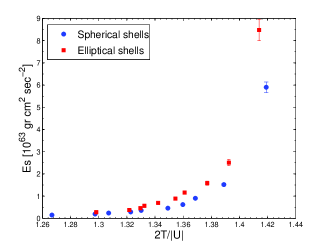
Figure 1.— Mean over halo surface pressure term vs. virial ratio at $z=0$. Blue circles are for spherical shells containing particles within 20% of the spherical $r_{\rm vir}$ shell, and red squares are for elliptical shells containing particles within 20% of the elliptical $r_{\rm vir}$ shell. The uncertainty was taken to be Poissonian, $\Delta<E_{\rm s}>=<E_{\rm s}>/\sqrt{N}$ where $N$ is the number of halos in the bin.

It is easy to see that the correction is larger in elliptical shells. Thus, for accurately using this proxy, using spherical shells maybe not good enough.

5. Results

5.1. Halos ellipticities at different relaxation levels

The axes ratios, $q$ and $s$, histograms for all halos are plotted in figure 2. In figures 3, 4, and 5 the relaxed and unrelaxed halos ellipticities are plotted for the three relaxation criteria, $r_{\rm offset}$, $2T/|U|$, and $(2T-Es)/|U|$, respectively. The values of the relaxation criteria were chosen such that in each plot both relaxed and unrelaxed samples have about the same number of halos, so the histograms will have a similar normalization.

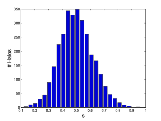
Figure 2.— Axes ratio histogram, where top and bottom panels are for $q$ and $s$ histograms, respectively.

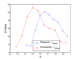
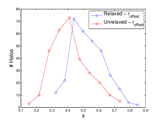
Figure 3.— Axes ratio histogram for halos in different relaxation level, when the distinction is made according to the $r_{\rm offset}$ criterion. The relaxed and unrelaxed samples have $r_{\rm offset}<0.02$ (315 halos) and $0.12\lesssim r_{\rm offset}<0.2$ (297 halos), respectively. Upper and lower panels are for $q$ and $s$ histograms, respectively.

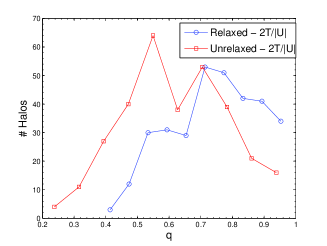
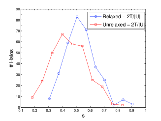
Figure 4.— Axes ratio histogram for halos in different relaxation level, when the distinction is made according to the $2T/|U|$ criterion. The relaxed and unrelaxed samples have $2T/|U|<1.25$ (326 halos) and $1.44\lesssim 2T/|U|<1.5$ (313 halos), respectively. Upper and lower panels are for $q$ and $s$ histograms, respectively.

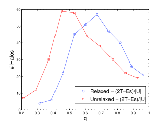
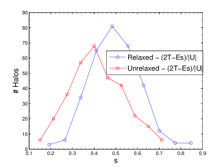
Figure 5.— Axes ratio histogram for halos in different relaxation level, when the distinction is made according to the $(2T-Es)/|U|$ criterion. The relaxed and unrelaxed samples have $(2T-Es)/|U|<0.95$ (319 halos) and $1.22\lesssim(2T-Es)/|U|<1.5$ (319 halos), respectively. Upper and lower panels are for $q$ and $s$ histograms, respectively.

Similar to figures 3 - 5, in figure 6 we plotted the fraction of relaxed clusters, $N_{\rm relaxed}/(N_{\rm relaxed}+N_{\rm unrelaxed})$, vs halo ellipticity. Here we took only halos with $q>0.4$ since more elliptical halos are rare and therefore give poor statistics. In addition, for halos with $q<0.4$ the values of both relaxation criteria are strongly dependent on the length of the ellipse major axis, which is likely due to the fact that many of them are in the process of a major merger and highly unrelaxed. The threshold was chosen so the three will have about the same normalization at $q=1$.

Figure 6.— Fraction of relaxed halos at different ellipticities and for different relaxation criteria, $2T/|U|=1.35$ (blue circles), $(2T-Es)/|U|=1.035$ (green squares), and $r_{\rm offset}=0.055$ (red asterisks). For these relaxation estimations we took halo particles within the elliptic virial radius. The uncertainties were taken to be Poissonian, i.e. $\Delta N_{\rm relaxed}=\sqrt{N_{\rm relaxed}}$ and $\Delta N_{\rm unrelaxed}=\sqrt{N_{\rm unrelaxed}}$.

The fraction of relaxed halos at different ellipticities is a little bit more sensitive to $r_{\rm offset}$ than to $2T/|U|$ and $(2T-Es)/|U|$.

In figure 7 we plotted $q$ vs $s$ at different relaxation level when relaxation is gauged by $r_{\rm offset}$, $2T/|U|$, and $(2T-Es)/|U|$ for the left, middle, and right panels, respectively. This is a convenient way to see the differences in the halos 3D shape between relaxed and unrelaxed halos.

Figure 7.— Triaxiality in different relaxation level and for different relaxation criteria. Left panel: Relaxation gauged by $r_{\rm offset}$, and the threshold value is the same as figure 3. Middle panel: Relaxation gauged by $2T/|U|$, and the threshold value is the same as figure 4. Right panel: Relaxation gauged by $(2T-Es)/|U|$, and the threshold value is the same as figure 5. The black solid line is for $q=s$. All halos are on one side of the black line since $q>s$ by definition (see § 3.1).

5.2. Averaged ellipticities vs main axes length

In figure 8 (top panel) we plotted the averaged $q$ and $s$ values over halos at $z=0$ at different portions of the virial radius for the semi-major axis. Only halos with a large number of particles, $>10^{3}$, inside the smallest radius, $0.5r_{\rm vir}$, were taken, which gave $\sim 10^{3}$ halos. We also plotted (bottom panel) the axes ratios for relaxed halos, $r_{\rm offset}<0.02$, which gave us 115 halos. The halo ellipticity first decreases a small amount, until $\sim(1.5-2)r_{\rm vir}$, then their ellipticity increases. In other words on average the halos are more elliptical at small radii then with increasing radius they become more spherical, and then elliptical again. This behavior is a little bit more pronounce in relaxed halos. However, the change is small, even in the relaxed sample, and over the radius range $(0.5-3)r_{\rm vir}$ the axes ratios are quite constant, $<q>\approx 0.66$ and $<s>\approx 0.5$ and $<q>\approx 0.7$ and $<s>\approx 0.54$, for the whole $\sim 10^{3}$ halo sample and for the relaxed one, respectively, especially compared to the large scatter.

Figure 8.— Profiles of the average axes ratio at $z=0$. Top panel: plotted are the average values of $q$ (solid curve) and $s$ (dashed curve), over all halos at volumes with a different semi-major axes value at $z=0$. Bottom panel: the same but only for relaxed halos, $r_{\rm offset}<0.02$. The central curves represent the mean value, with the $\pm$ 1–$\sigma$ width of the distribution uncertainty around the mean is marked by the upper and lower curves.

5.3. The DM velocity anisotropy profile

To assess the impact of an aspherical halo configuration, we plot in figure 9 the velocity anisotropy profiles in both spherical and elliptical shells for all high-mass halos ($M_{\rm vir}\geqslant 10^{14}$ h${}^{-1}_{0.7}$ M_⊙).

Figure 9.— Velocity anisotropy profiles when the shells are described as spherical (red dash curves) or elliptical (blue solid curves). Note, the radius in the elliptical case is the semi-major axis. The central curves represent the mean value, with the $\pm$ 1–$\sigma$ uncertainty around the mean is marked by the upper and lower curves. The green squares are averaged values of 16 clusters, when $\beta$ was inferred from X-ray observations (Host e.t al. 2009). The black triangle is a value inferred for A1689 using galaxy dynamics information (Lemze et al. 2011).

It is interesting to note that the average $\beta$ profile is almost the same in spherical and elliptical shells till $\sim(0.7-1)r_{\rm vir}$. Beyond this region, however, the scatter of $\beta$ using elliptical shells is much smaller. On top of the theoretical expectation we plotted the $\beta$ values estimated indirectly from data. The green squares are averaged values of 16 clusters, when $\beta$ was inferred from X-ray observations (Host e.t al. 2009). The black triangle is a value inferred for A1689 using galaxy dynamics information (Lemze et al. 2011).

Average DM velocity anisotropy profiles of all high-mass halos, $M_{\rm vir}\geqslant 10^{14}$ h${}^{-1}_{0.7}$ M_⊙, are plotted in figure 10 (including 1$\sigma$ uncertainty regions) for different redshifts and for spherical and elliptical shells. Using spherical shells, the profiles are essentially similar at small radii, $r\lesssim 0.3r_{\rm vir}$, roughly independent of redshift. However, at larger radii, $r\sim 0.7r_{\rm vir}$, values of $\beta$ are somewhat higher in high redshift halos. At even larger radii, $r\gtrsim r_{\rm vir}$, $\beta$ is lower at higher redshifts. As the redshift increases, the scatter in $\beta$ increases as a function of radius from $\sim 0.3r_{\rm vir}$. Using elliptical shells, the differences between the profiles decrease.

Figure 10.— Velocity anisotropy profiles at different redshifts. Left panel: using spherical shells. Middle panel: the relatively small variation of the anisotropy in the region $0-1$ $r_{\rm vir}$ in spherical shells is shown separately. Right panel: using elliptical shells, with elliptical radii, $r_{\rm e}$, scaled by $r_{\rm vir}$ of the spherical radius.

In figure 11 we illustrate the DM velocity anisotropy profiles for two mass ranges in spherical and elliptical shells, respectively. The 100 most massive halos, $M\gtrsim 10^{15}$ h${}_{0.7}^{-1}$ M_⊙, and least massive halos, $M\sim 10^{14}$ h${}_{0.7}^{-1}$ M_⊙, are compared at redshift $z=0$.

Figure 11.— Velocity anisotropy profiles of halos with different masses. Profiles of the 100 most (solid curve), $M\gtrsim 10^{15}$ h${}_{0.7}^{-1}$ M_⊙, and least (dashed curve), $M\sim 10^{14}$ h${}_{0.7}^{-1}$ M_⊙, massive halos at $z=0$ in spherical shells.

As mentioned in § 4, there are various criteria for relaxed clusters. Here we use the $r_{\rm offset}$ criterion, since the difference between the relaxed and unrelaxed $\beta$ profiles is the largest (among the first three). We also mentioned in § 4, the threshold values of the (quantitative) criteria according to which halos are classified as relaxed or unrelaxed are quite arbitrary. However, in § A we can see that $r_{\rm offset}$ is more correlate with the halo ellipticity (which relates to the relaxation level, see § 5.1) than the virial and corrected virial ratio. We chose in our analysis to compare among the $\beta$ profiles by setting two comparable numbers corresponding to the most and least relaxed phases.

Figure 12.— Velocity anisotropy profiles of relaxed (blue solid curves) and unrelaxed (red dashed curves) halos analyzed in spherical shells. Relaxation gauged by the $r_{\rm offset}$ criterion: relaxed and unrelaxed halos have $r_{\rm offset}<0.015$ (264 halos) and $r_{\rm offset}>0.17$ (267 halos), respectively.

In figure 12 we plot the velocity anisotropy profile of relaxed versus unrelaxed halos using spherical shells when the distinction is made according to the $r_{\rm offset}$ criterion, where relaxed and unrelaxed halos have $r_{\rm offset}<0.015$ (264 halos) and $r_{\rm offset}>0.17$ (267 halos), respectively. Using the virial ratio to distinguish between relaxed and unrelaxed halos yielded very similar $\beta$ profiles, and therefore these are not shown here. At radii smaller than the virial radius applying the $r_{\rm offset}$ criterion results in flattened velocity anisotropy profiles of the unrelaxed halos with respect to the relaxed halos.

The $\beta$ profile of relaxed versus unrelaxed halos in elliptical shells are not appreciably different than the ones using spherical shells.

Figure 13.— Velocity anisotropy profiles of relaxed (blue solid curves) and unrelaxed (red dashed curves) halos in elliptical shells. Relaxation gauged by the $r_{\rm offset}$ criterion: relaxed and unrelaxed halos have $s_{\rm offset}<0.019$ (273 halos) and $r_{\rm offset}>0.13$ (283 halos), respectively.

In figure 13 we plot the velocity anisotropy profile of relaxed versus unrelaxed halos using elliptical shells when the distinction is made according to the $r_{\rm offset}$ criterion. The profiles are similar to those for spherical shells except for a smaller decline and with a smaller scatter at large radii. Here we can also check if the indication that $r_{\rm offset}$ is a better relaxation proxy depends on the chosen threshold values. The correlations between all of the five criteria and halos ellipticities are shown in § A. Out of the three relaxation criteria we focused ($r_{\rm offset}$, $2T/|U|$, and $(2T-Es)/|U|$), the correlation between $r_{\rm offset}$ and the halos ellipticities is the highest. Therefore, we conclude that our findings do not depend on the threshold value.

5.4. $\gamma$-$\beta$ ratio

As was mentioned in § 1, the question of whether $\gamma$ and $\beta$ are correlated is of both theoretical and practical interest. In figure 14 we show the velocity anisotropy vs. the radial density slope for all shells in all halos (left panel), all shells of relaxed halos according to the virial relation criterion $2T/|U|<1.35$ (middle panel), and all shells of highly relaxed halos with $2T/|U|<1.35$ and $r_{\rm offset}<0.025$ (right panel). For each halo we checked the maximum grid level and determined the halo minimum spatial resolution. Unresolved shells were not included in the analysis. The black curve reproduces the Hansen & Moore relation, $\beta(\gamma)=1-1.15(1+\gamma/6)$, for the $-4<\gamma<0$ range. In figure 15 we drew the same quantities for all shells in all halos, assuming NFW-distributed density profiles. Red circles with error bars show the median anisotropy profile and $1\sigma$ dispersion. Note that in this plot the $\gamma$ range is $(\sim-2.9,-1)$, not ($-3$,$-1$), due to the finite binned values of the radius.

Figure 14.— Velocity anisotropy vs. radial density slope at $z=0$. Plotted are values corresponding to all shells and halos (left panel), all shells of relaxed halos according to the virial relation criterion $2T/|U|<1.35$ (middle panel), and all shells of highly relaxed halos, specified by $2T/|U|<1.35$ and $r_{\rm offset}<0.025$ (right panel). The HM06 relation is plotted in the $-4<\gamma<0$ range (black solid curve).

Figure 15.— Velocity anisotropy vs. radial density slope at $z=0$. Plotted are values for all shells and halos, with $\gamma$ inferred from an NFW fit (blue dots). Red circles with error bars show the median anisotropy profile and $1\sigma$ dispersion. The HM06 relation is plotted in the $-4<\gamma<0$ range (black solid curve).

Finally, figure 16 describes the velocity anisotropy against the radial density slope of the four inner ($0<r<0.3r_{\rm vir}$, top panel) and all the other ($0.3r_{\rm vir}<r<r_{\rm vir}$, bottom panel) shells. This boundary value was chosen since shells included within this radius, $0.3r_{\rm vir}$, display the strongest $\gamma$-$\beta$ correlation. In the panel showing values for the inner shells we also plotted red circles with error bars that show the median anisotropy profile and $1\sigma$ dispersion.

Figure 16.— Velocity anisotropy vs. radial density slope at $z=0$. Top panel: plotted are values for the four inner shells, $0<r<0.3r_{\rm vir}$, and red circles with error bars show the median anisotropy profile and $1\sigma$ dispersion. Bottom panel: values for the outer shells, $0.3r_{\rm vir}<r<r_{\rm vir}$. The HM06 relation is depicted in the $-4<\gamma<0$ range (black solid curve). The vertical line at $\gamma\simeq-2$ is an artifact due to the fact that $\gamma$ here is a discrete slope profile calculated between two bins with a low number of particles. This artifact can also be seen in figure 14, though it is more prominent here.

We have made two checks in order to see if our results are different when there is a higher number of particles in each shell. First we decreased the number of bins from 15 per virial radius to 5. The main effect was a decrease in the $\gamma$ value range. This can be due to the fact that with a lower number of bins the minimum and maximum bins are closer and the mean has lower variance. In the second test we checked the 100 most massive halos, which obviously have higher number of particles per shell than the full sample. In both cases the correlation between $\beta$ and $\gamma$ did not increase significantly, as can be seen in figure 17 for the $\beta$ and $\gamma$ plot of the 100 most massive halos.

Figure 17.— Velocity anisotropy vs. radial density slope at $z=0$ for the 100 most massive halos.

As expected, since the $\beta$ values were taken within the virial radius, and since their largest difference between spherical and elliptical shells is at $r>r_{\rm vir}$, when we repeated this above analysis with triaxial halos, the results were essentially the same as those obtained for spherical halos.

6. Discussion

Significant progress has recently been made in the ability to deduce the kinematic properties of DM in clusters from galaxy dynamics and X-ray measurements. Comparison of these properties with results from numerical simulations can clearly test analysis methods and add new insights on DM phase space occupation. We presented results from an analysis of DM velocities in $6019$ halos with masses $M\geqslant 10^{14}$ h${}_{0.7}^{-1}$ M_⊙ at redshift $z=0$, drawn from one of the largest ever hydrodynamic cosmological AMR simulations.

We found that each halo ellipticity depends strongly on the major axis length. This is because for each halo ellipsoids with different sizes include different parts of substructure and infalling clumps, which obviously affect the ellipticity, if they are inside or close to the ellipse. However, averaging over many halos, $\sim 10^{3}$, the halo ellipticity first decreases a small amount, until $\sim(1.5-2)r_{\rm vir}$, then the averaged ellipticity increases. In other words on average the halos are more elliptical at small radii then with increasing radius they become more spherical, and then elliptical again, since at large radii other structures are located inside the ellipsoid and this on average increases the ellipticity. However, the change is small, even in the relaxed sample, and over the radius range $(0.5-3)r_{\rm vir}$ the axis ratios are essentially constant, $<q>\approx 0.66$ and $<s>\approx 0.5$ and $<q>\approx 0.7$ and $<s>\approx 0.54$, for the whole $\sim 10^{3}$ halo sample and for the relaxed one, respectively, especially compared to the large scatter. This ellipticity vs radius behavior is in agreement with Allgood et al. (2006) who found that halos become more spherical up to $r=r_{\rm vir}$, and Bailin & Steinmetz (2005), who found the ellipticity is quite constant compared with the scatter. Kuhlen et al. (2007), Hayashi et al. (2007), and Vera-Ciro et al. (2011) used various N-body simulations and found that, similarly to cluster-size halos, in galaxy-size halos the core is more elliptical than a few hundreds of kpc away. However, Hopkins, Bahcall, & Bode (2005) found that cluster cores are less elliptical than cluster outskirts

We have employed five different relaxation criteria and focused on three of them, $r_{\rm offset}$, $2T/|U|$, and $(2T-Es)/|U|$; see the Appendix for the correlations of these three with the two other relaxation proxies we also considered. Relaxed halos tend to be more spherical while unrelaxed halos tend to be more prolate. This is seen using various relaxation criteria, e.g. $r_{\rm offset}$, $2T/|U|$, $(2T-Es)/|U|$. This can be explained by the evolution of clusters from highly aligned and elongated systems at early times to lower alignment and elongation at present, which reflects the hierarchical and filamentary nature of structure formation (Hopkins, Bahcall, & Bode 2005). Indeed, Vera-Ciro et al. (2011), who analyzed Aquarius data, found that $q$ increases with time. This is also in agreement with Shaw et al. (2006) who found that low mass halos, which are older than their higher mass counterparts and therefore had a longer time to relax dynamically, attain a more spherical morphology than high mass halos.

Our study indicates that the profiles of cluster DM velocity anisotropy have a similar pattern when these are averaged over all halo masses, redshifts, and relaxation stages, even though there is a considerable scatter in magnitude due to the large differences in the $\beta$ profile of individual halos. A typical behavior is a rising $\beta$ profile from a nearly vanishing central value, leveling off at $r\sim 0.2r_{\rm vir}$, out to large radii of at least $(1.5-2)r_{\rm vir}$. This plateau is clearer in elliptical shells and at lower redshifts. The rising value from zero at small radii behavior is in agreement with previous works (e.g. Crone et al. 1994; Tormen et al. 1997; Thomas et al. 1998; Eke et al. 1998;Colin et al. 2000; Rasia et al. 2004). Interestingly, Lau, Nagai, & Kravtsov (2010) showed that the inclusion of radiative cooling and star formation in the simulation slightly lowers the $\beta$ values at $z=0$ but not at $z=1$. Unrelaxed halos have lower $\beta$ values, which indicates that the DM particles infall is less radial than in relaxed halos. Lower mass halos have, on average, lower $\beta$ levels at $r=r_{\rm vir}$, and therefore even shallower profiles. This behavior could possibly be due to the ability to reach higher accretion velocities at lower redshifts when the background density is much lower. However, our mass range, especially in elliptical shells, is very small, so these findings are preliminary.

Some effort is now devoted to determine $\beta$ either by using the gas temperature as a tracer of it, a method which was applied for 16 clusters at intermediate radii (Host et al. 2009), or by examining galaxy velocities, as has recently been demonstrated in the analysis of A1689 measurements (Lemze et al. 2011). Interestingly, these indirect measurements of $\beta$ fall on the upper end of the theoretically expected range. Both methods assume steady state, i.e. $\overline{v}_{r}=0$. Clusters on the other hand are not in steady state, since matter is continuously falling onto them. However, at small radii (the indirect measurements radii range), i.e. $r\lesssim 0.7$ $r_{\rm vir}$, this effect on $\beta$ is negligible, $\lesssim 4\%$. In a recent work, Peter, Moody, & Kamionkowski (2010) used simulations and showed that for galaxy-size halos, the expected $\beta$ increases with radius till about the virial radius when DM particles decay to a slightly less massive particle with a large decaying time, $\tau\gtrsim$ a few Gyr, and a high velocity kick, $v_{\rm kick}\gtrsim 150$ km s^-1.

Lastly, we find that there is some correlation between $\gamma$ and $\beta$ at low radii, $r<0.3r_{\rm vir}$, and that such a correlation can be induced at all radii merely by assuming a prescribed DM density profile (since when assuming a profile the $\gamma$ values are correlated and therefore the scatter along the $\gamma$ axis is reduced). The level of $\gamma$ – $\beta$ correlation is very low at large radii, $r>0.3r_{\rm vir}$, even for very relaxed halos. Repeating the same analysis with elliptical shells led to the same result. Indeed, most of the works that try to explain the relation between $\gamma$ and $\beta$ focus on the inner regions. Hansen et al. (2005) and Hansen (2009) assumed spherically symmetric systems in hydrostatic equilibrium, and that high energy tail of the tangential velocity distribution function follows that of the radial velocity distribution function, based on which they explain the $\gamma$-$\beta$ relation mainly at small radii where both $\gamma$ and $\beta$ are about zero. An & Evans (2006, and references therein) have deduced that $\gamma\leq\beta$. Ciotti & Morganti (2010) claimed that this inequality holds not only at the center, but also at larger radii in a very large class of spherical systems whenever the phase-space distribution function is positive.

7. Conclusions

Our main conclusions are as follows:

• Galaxy clusters are generally triaxial.

• Relaxed halos tend to be more spherical while unrelaxed halos tend to be more prolate.

• Low mass halos tend to be more relaxed (see § A), though this result is based on a narrow mass range and therefore should be considered preliminary.

• The ellipticity of each halo strongly depends on the semi-major axis amplitude. However, averaging over many halos, $\sim 10^{3}$, there is no significant difference in the ellipticity at ellipses with different semi-major axis amplitudes, even in the relaxed sample.

• The $r_{\rm offset}$ is a better relaxation proxy than $2T/|U|$ and $(2T-Es)/|U|$ in the sense that its correlation with the halo ellipticity is stronger.

• The pressure term, $Es$, is larger in elliptical sells and in less relaxed halos (when the relaxation criterion is $2T/|U|$).

• DM velocity anisotropy profiles have a similar pattern when these are averaged over all halo masses, redshifts, triaxiality, and relaxation stages, even though there is a considerable scatter in magnitude due to the large differences in the $\beta$ profile of individual halos. A typical behavior is a rising $\beta$ profile from a nearly vanishing central value, leveling off at $r\sim 0.2r_{\rm vir}$, out to large radii of at least $(1.5-2)r_{\rm vir}$. This plateau is clearer in elliptical shells and at lower redshifts.

• DM velocity anisotropy indirect measurements fall on the upper end of the theoretically predicted range.

• There is some correlation between $\gamma$ and $\beta$ at low radii, $r<0.3r_{\rm vir}$, and that such a correlation can be induced at all radii merely by assuming a prescribed DM density profile. The level of $\gamma$ – $\beta$ correlation is very low at large radii, $r>0.3r_{\rm vir}$, even for very relaxed halos.

The average expected DM velocity anisotropy has a similar pattern for all halo masses, redshifts, triaxiality, and relaxation stages. DM velocity anisotropy indirect measurements fall on the upper edge of the theoretical expectations (see figure 9). Though measured indirectly, the estimations are derived by using two different surrogate measurement, i.e. X-ray and galaxy dynamics. So far the DM velocity anisotropy estimates were based on a very low number of clusters (16 via X-ray and 1 via galaxy dynamics). It will be important to contrast the theoretically predicted values with results from a larger cluster sample. We plan to do this in CLASH.

Appendix A The correlations between the axes ratios, relaxation proxies, and $\beta$

Here we present the correlations between the axes ratios $q$, $s$, relaxation proxies $r_{\rm offset}$, $r_{\rm sub}$, $r_{\rm dp}$, $2T/|U|$, $(2T-Es)/|U|$ (when $Es$ is estimated by the outer 20% and 10% shell volume for comparison). In tables 1 and 2 the correlations are calculated out of all the halos and the ones with $q\geqslant 0.4$, respectively.

Table 1Correlations Matrix - All halos

	$M_{\rm vir}$	$q$	$s$	$r_{\rm offset}$	$r_{\rm sub}$	$r_{\rm dp}$	$2T/|U|$	$(2T-E_{s,20\%})/|U|$,20%	$(2T-Es)/|U|$,10%
$M_{\rm vir}$	1	-0.26	-0.24	0.15	0.14	0	0.28	0.11	0.1
$q$	-0.26	1	0.75	-0.32	-0.33	-0.08	-0.21	-0.16	-0.16
$s$	-0.24	0.75	1	-0.38	-0.39	-0.1	-0.23	-0.17	-0.17
$r_{\rm offset}$	0.15	-0.32	-0.38	1	0.86	0.21	0.38	-0.09	-0.09
$r_{\rm sub}$	0.14	-0.33	-0.39	0.86	1	0.28	0.38	-0.06	-0.06
$r_{\rm dp}$	0	-0.08	-0.1	0.21	0.28	1	0.09	0.1	0.09
$2T/|U|$	0.28	-0.21	-0.23	0.38	0.38	0.09	1	0.41	0.31
$(2T-Es)/|U|$,20%	0.11	-0.16	-0.17	-0.09	-0.06	0.1	0.41	1	0.96
$(2T-Es)/|U|$,10%	0.1	-0.16	-0.17	-0.09	-0.06	0.09	0.31	0.96	1

Table 2Correlations Matrix - Halos with $q\geqslant 0.4$

	$M_{\rm vir}$	$q$	$s$	$r_{\rm offset}$	$r_{\rm sub}$	$r_{\rm dp}$	$2T/|U|$	$(2T-Es)/|U|$,20%	$(2T-Es)/|U|$,10%
$M_{\rm vir}$	1	-0.23	-0.21	0.13	0.1	-0.05	0.26	0.09	0.08
$q$	-0.23	1	0.71	-0.24	-0.23	0.02	-0.15	-0.11	-0.12
$s$	-0.21	0.71	1	-0.32	-0.31	-0.03	-0.16	-0.12	-0.13
$r_{\rm offset}$	0.13	-0.24	-0.32	1	0.85	0.22	0.35	-0.14	-0.14
$r_{\rm sub}$	0.1	-0.23	-0.31	0.85	1	0.22	0.33	-0.14	-0.13
$r_{\rm dp}$	-0.05	0.02	-0.03	0.22	0.22	1	0.02	0.04	0.04
$2T/|U|$	0.26	-0.15	-0.16	0.35	0.33	0.02	1	0.38	0.27
$(2T-Es)/|U|$,20%	0.09	-0.11	-0.12	-0.14	-0.14	0.04	0.38	1	0.96
$(2T-Es)/|U|$,10%	0.08	-0.12	-0.13	-0.14	-0.13	0.04	0.27	0.96	1

References

- Allgood et al. (2006) Allgood, B., Flores, R. A., Primack, J. R., Kravtsov, A. V., Wechsler, R. H., Faltenbacher, A., & Bullock, J. S. 2006, MNRAS , 367, 1781
- An & Evans (2006) An, J. H., & Evans, N. W. 2006, ApJ , 642, 752
- Arnaud et al. (2005) Arnaud, M., Pointecouteau, E., & Pratt, G. W. 2005, A&A , 441, 893
- Atrio-Barandela et al. (2008) Atrio-Barandela, F., Kashlinsky, A., Kocevski, D., & Ebeling, H. 2008, ApJ , 675, L57
- Bailin & Steinmetz (2005) Bailin, J., & Steinmetz, M. 2005, ApJ , 627, 647
- Ballesteros-Paredes (2006) Ballesteros-Paredes, J. 2006, MNRAS , 372, 443
- Benatov et al. (2006) Benatov, L., Rines, K., Natarajan, P., Kravtsov, A., & Nagai, D. 2006, MNRAS , 370, 427
- Binney & Tremaine (2008) Binney, J., & Tremaine, S. 2008, Galactic Dynamics: Second Edition, by James Binney and Scott Tremaine. ISBN 978-0-691-13026-2 (HB). Published by Princeton University Press, Princeton, NJ USA, 2008.,
- Broadhurst et al. (2005a) Broadhurst, T., et al. 2005, ApJ , 621, 53 (B05a)
- Broadhurst et al. (2005b) Broadhurst, T., Takada, M., Umetsu, K., Kong, X., Arimoto, N., Chiba, M., & Futamase, T. 2005, ApJ , 619, L143 (B05b)
- Broadhurst et al. (2008) Broadhurst, T., Umetsu, K., Medezinski, E., Oguri, M., & Rephaeli, Y. 2008, ApJ , 685, L9
- Bryan & Norman (1997) Bryan, G. L., & Norman, M. L. 1997, Computational Astrophysics; 12th Kingston Meeting on Theoretical Astrophysics, 123, 363
- Bryan & Norman (1998) Bryan, G. L., & Norman, M. L. 1998, ApJ , 495, 80
- Carlberg et al. (1997) Carlberg, R. G., et al. 1997, ApJ , 485, L13
- Chandrasekhar (1961) Chandrasekhar, S. 1961, International Series of Monographs on Physics, Oxford: Clarendon
- Ciotti & Morganti (2010) Ciotti, L., & Morganti, L. 2010, MNRAS , 408, 1070
- Cole & Lacey (1996) Cole, S., & Lacey, C. 1996, MNRAS , 281, 716
- Colín et al. (2000) Colín, P., Klypin, A. A., & Kravtsov, A. V. 2000, ApJ , 539, 561
- Crone et al. (1994) Crone, M. M., Evrard, A. E., & Richstone, D. O. 1994, ApJ , 434, 402
- Davis et al. (2011) Davis, A. J., D’Aloisio, A., & Natarajan, P. 2011, MNRAS , 416, 242
- Diaferio & Geller (1997) Diaferio, A., & Geller, M. J. 1997, ApJ , 481, 633
- Diaferio (1999) Diaferio, A. 1999, MNRAS , 309, 610
- Diaferio et al. (2005) Diaferio, A., Geller, M. J., & Rines, K. J. 2005, ApJ , 628, L97
- Diemand et al. (2004) Diemand, J., Moore, B., & Stadel, J. 2004, MNRAS , 352, 535
- Dubinski & Carlberg (1991) Dubinski, J., & Carlberg, R. G. 1991, ApJ , 378, 496
- Einasto (1965) Einasto J., 1965, Trudy Inst. Astroz. Alma-Ata, 51, 87
- Eisenstein & Hut (1998) Eisenstein, D. J., & Hut, P. 1998, ApJ , 498, 137
- Eisenstein & Hu (1999) Eisenstein, D. J., & Hu, W. 1999, ApJ , 511, 5
- Eke et al. (1998) Eke, V. R., Navarro, J. F., & Frenk, C. S. 1998, ApJ , 503, 569
- Hallman et al. (2007) Hallman, E. J., O’Shea, B. W., Burns, J. O., Norman, M. L., Harkness, R., & Wagner, R. 2007, ApJ , 671, 27
- Hansen et al. (2005) Hansen, S. H., Egli, D., Hollenstein, L., & Salzmann, C. 2005, NewA , 10, 379
- Hansen & Moore (2006) Hansen, S. H., & Moore, B. 2006, New Astronomy, 11, 333
- Hansen & Stadel (2006) Hansen, S. H., & Stadel, J. 2006, JCAP , 5, 14
- Hansen (2009) Hansen, S. H. 2009, ApJ , 694, 1250
- Hayashi et al. (2007) Hayashi, E., Navarro, J. F., & Springel, V. 2007, MNRAS , 377, 50
- Hopkins et al. (2005) Hopkins, P. F., Bahcall, N. A., & Bode, P. 2005, ApJ , 618, 1
- Host et al. (2009) Host, O., Hansen, S. H., Piffaretti, R., Morandi, A., Ettori, S., Kay, S. T., & Valdarnini, R. 2009, ApJ , 690, 358
- Jing et al. (1995) Jing, Y. P., Mo, H. J., Borner, G., & Fang, L. Z. 1995, MNRAS , 276, 417
- Jing & Suto (2002) Jing, Y. P., & Suto, Y. 2002, ApJ , 574, 538
- Katz (1991) Katz, N. 1991, ApJ , 368, 325
- Kuhlen et al. (2007) Kuhlen, M., Diemand, J., & Madau, P. 2007, ApJ , 671, 1135
- Lau et al. (2010) Lau, E. T., Nagai, D., & Kravtsov, A. V. 2010, ApJ , 708, 1419
- Lemze et al. (2008) Lemze, D., Barkana, R., Broadhurst, T. J., & Rephaeli, Y. 2008, MNRAS , 386, 1092
- Lemze et al. (2009) Lemze, D., Broadhurst, T., Rephaeli, Y., Barkana, R., & Umetsu, K. 2009, ApJ , 701, 1336
- Lemze et al. (2011) Lemze, D., Rephaeli, Y., Barkana, R., Broadhurst, T., Wagner, R., & Norman, M. L. 2011, ApJ , 728, 40
- Limousin et al. (2007) Limousin, M., et al. 2007, ApJ , 668, 643
- Ludlow et al. (2011) Ludlow, A. D., Navarro, J. F., White, S. D. M., et al. 2011, MNRAS , 415, 3895
- McKee & Zweibel (1992) McKee, C. F., & Zweibel, E. G. 1992, ApJ , 399, 551
- Medezinski et al. (2007) Medezinski, E., et al. 2007, ApJ , 663, 717
- Moore et al. (1998) Moore, B., Governato, F., Quinn, T., Stadel, J., & Lake, G. 1998, ApJ , 499, L5
- Navarro et al. (1997) Navarro, J. F., Frenk, C. S., & White, S. D. M. 1997, ApJ , 490, 493
- Navarro et al. (2010) Navarro, J. F., et al. 2010, MNRAS , 402, 21
- Neto et al. (2007) Neto, A. F., et al. 2007, MNRAS , 381, 1450
- Norman & Bryan (1999) Norman, M. L., & Bryan, G. L. 1999, Numerical Astrophysics, 240, 19
- Norman et al. (2007) Norman, M. L., Bryan, G. L., Harkness, R., Bordner, J., Reynolds, D., O’Shea, B., & Wagner, R. 2007, arXiv:0705.1556
- Peter et al. (2010) Peter, A. H. G., Moody, C. E., & Kamionkowski, M. 2010, Phys. Rev. D. , 81, 103501
- Pointecouteau et al. (2005) Pointecouteau, E., Arnaud, M., & Pratt, G. W. 2005, A&A , 435, 1
- Postman et al. (2011) Postman, M., et al. 2012, ApJS , 199, 25
- Rasia et al. (2004) Rasia, E., Tormen, G., & Moscardini, L. 2004, MNRAS , 351, 237
- Schmidt & Allen (2007) Schmidt, R. W., & Allen, S. W. 2007, MNRAS , 379, 209
- Shaw et al. (2006) Shaw, L. D., Weller, J., Ostriker, J. P., & Bode, P. 2006, ApJ , 646, 815
- Tissera et al. (2010) Tissera, P. B., White, S. D. M., Pedrosa, S., & Scannapieco, C. 2010, MNRAS , 406, 922
- Thomas et al. (1998) Thomas, P. A., Colberg, J. M., Couchman, H. M. P., et al. 1998, MNRAS , 296, 1061
- Thomas et al. (2001) Thomas, P. A., Muanwong, O., Pearce, F. R., Couchman, H. M. P., Edge, A. C., Jenkins, A., & Onuora, L. 2001, MNRAS , 324, 450
- Tormen et al. (1997) Tormen, G., Bouchet, F. R., & White, S. D. M. 1997, MNRAS , 286, 865
- Umetsu et al. (2010) Umetsu, K., Medezinski, E., Broadhurst, T., Zitrin, A., Okabe, N., Hsieh, B.-C., & Molnar, S. M. 2010, ApJ , 714, 1470
- Vera-Ciro et al. (2011) Vera-Ciro, C. A., Sales, L. V., Helmi, A., Frenk, C. S., Navarro, J. F., Springel, V., Vogelsberger, M., & White, S. D. M. 2011, arXiv:1104.1566
- Vikhlinin et al. (2006) Vikhlinin, A., Kravtsov, A., Forman, W., Jones, C., Markevitch, M., Murray, S. S., & Van Speybroeck, L. 2006, ApJ , 640, 691
- Voit (2005) Voit, G. M. 2005, Reviews of Modern Physics, 77, 207
- Wang & White (2009) Wang, J., & White, S. D. M. 2009, MNRAS , 396, 709
- Warren et al. (1992) Warren, M. S., Quinn, P. J., Salmon, J. K., & Zurek, W. H. 1992, ApJ , 399, 405
- Wojtak et al. (2005) Wojtak, R., Łokas, E. L., Gottlöber, S., & Mamon, G. A. 2005, MNRAS , 361, L1
- Zemp et al. (2011) Zemp, M., Gnedin, O. Y., Gnedin, N. Y., & Kravtsov, A. V. 2011, ApJS , 197, 30
- Zitrin et al. (2009) Zitrin, A., et al. 2009, MNRAS , 396, 1985
- Zitrin et al. (2010) Zitrin, A., et al. 2010, MNRAS , 408, 1916
- Zitrin et al. (2011) Zitrin, A., Broadhurst, T., Coe, D., et al. 2011, ApJ , 742, 117