Lorentz noninvariant oscillations of massless neutrinos are excluded

Abstract

The bicycle model of Lorentz noninvariant neutrino oscillations without neutrino masses naturally predicts maximal mixing and a $1/E$ dependence of the oscillation argument for $\nu_{\mu}\to\nu_{\tau}$ oscillations of atmospheric and long-baseline neutrinos, but cannot also simultaneously fit the data for solar neutrinos and KamLAND. Within the Standard Model Extension, we examine all 19 possible structures of the effective Hamiltonian for Lorentz noninvariant oscillations of massless neutrinos that naturally have a $1/E$ dependence at high neutrino energy. Due to the lack of any evidence for direction dependence, we consider only direction-independent oscillations. Although we find a number of models with a $1/E$ dependence for atmospheric and long-baseline neutrinos, none can also simultaneously fit solar and KamLAND data.

1 Introduction

Neutrino data from atmospheric, long-baseline, solar and reactor experiments are easily explained by oscillations of three active, massive neutrinos [1]. Lorentz-invariance and $CPT$ violating interactions originating at the Planck scale can also lead to neutrino oscillations. The Standard Model Extension (SME) [2] includes all such interactions that may arise from spontaneous symmetry breaking but still preserve Standard Model gauge invariance and power-counting renormalizability. Studies of neutrino oscillations with Lorentz invariance violation have been made both for massive [3, 4, 5] and massless [6, 7, 8] neutrinos. A model with nonrenormalizable Lorentz invariance violating interactions and neutrino mass has also been proposed [9]. However, no viable model has been found that does not require at least one nonzero neutrino mass. The purpose of this paper is to determine if Lorentz invariance violation alone can account for the verified oscillation phenomena seen in atmospheric, long-baseline, solar and reactor neutrinos. We do not attempt to fit the possible oscillation signals seen in the LSND [10] and MiniBooNE [11] experiments.

In the SME, the evolution of massless neutrinos in vacuum may be described by the effective Hamiltonian [6]

$$(h_{eff})_{ij}=E\delta_{ij}+{1\over E}\left[a_{L}^{\mu}p_{\mu}-c_{L}^{\mu\nu}p_{\mu}p_{\nu}\right]_{ij}\,,$$ (1)

where $p_{\mu}=(E,-E\hat{p})$ is the neutrino four-momentum, $\hat{p}$ is the neutrino direction, $i,j$ are flavor indices, and $a_{L}\to-a_{L}$ for antineutrinos. The coefficients $a_{L}$ have dimensions of energy and the $c_{L}$ are dimensionless. Direction dependence of the neutrino evolution enters via the space components of $a_{L}$ and $c_{L}$, $\mu$ or $\nu=X,Y,Z$, while direction independent terms have $\mu=\nu=T$. The Kronecker delta term on the right-hand side of Eq. (1) may be ignored since oscillations are insensitive to terms in $h_{eff}$ proportional to the identity.

The two-parameter bicycle model [6] can be defined as follows: $(c_{L})_{ij}$ has only one nonzero element in flavor space and the only nonzero $(a_{L})_{ij}$ are $(a_{L})_{e\mu}=(a_{L})_{e\tau}$. These interactions can be nonisotropic, which could lead to different oscillation parameters for neutrinos propagating in different directions. In Ref. [8] it was shown that the pure direction-dependent bicycle model is ruled out by solar neutrino data alone, while a combination of atmospheric, solar and long-baseline neutrino data excludes the pure direction-independent case. A mixture of direction-dependent and direction-independent terms (with 5 parameters) is also excluded when KamLAND data are added [8].

The key feature of the bicycle model is that even though the terms in $h_{eff}$ are either constant or proportional to neutrino energy, at high neutrino energies there is a seesaw type mechanism that leads to $1/E$ behavior for the oscillation argument for atmospheric and long-baseline neutrinos. In this paper we examine the general case of direction-independent Lorentz invariance violation in the Standard Model Extension for three neutrinos without neutrino mass, i.e., Eq. (1) with only $c_{L}^{TT}$ and $a_{L}^{T}$ terms. We do not consider possible direction-dependent terms since there is no evidence for direction dependence in neutrino oscillation experiments (see, e.g., the experiments in Ref. [12] and the analysis of Ref. [6]). For notational simplicity we henceforth drop the $L$ subscript and $T$ superscripts from the $c_{L}^{TT}$ and $a_{L}^{T}$ in our formulae.

We first look for textures of the $c_{ij}$ in flavor space that allow a $1/E$ dependence of the oscillation argument at high neutrino energy. We then check the phenomenology for atmopheric, long-baseline, solar and reactor neutrino experiments. We were unable to find any texture of $h_{eff}$ that could simultaneously fit all the data.

In Sec. 2 we review the constraints on the direction-independent bicycle model. In Sec. 3 we list all possible textures of the $c$ coefficients and find which ones allow a $1/E$ dependence of the oscillation argument at high neutrino energies. For those that do, we first check the oscillation amplitude for atmospheric and long-baseline neutrinos, and if suitable parameters are found we then check the ability of the model to fit KamLAND and solar neutrino data. In Sec. 4 we summarize our results.

2 Neutrino oscillations in the bicycle model

As an illustrative analysis, we begin with a review of the direction-independent bicycle model and show how it is inconsistent with a combination of atmospheric, long-baseline and solar neutrino data.

Neutrino oscillations occur due to eigenenergy differences in $h_{eff}$ and the fact that the neutrino flavor eigenstates are not eigenstates of $h_{eff}$. In our generalization of the direction-independent bicycle model,

$$h_{eff}=\pmatrix{-2cE+2a_{11}&a_{12}&a_{13}\cr a_{12}&0&0\cr a_{13}&0&0}\,,$$ (2)

where the $c$ term is $CPT$-even and the $a_{ij}$ terms are $CPT$-odd. The simple two-parameter bicycle model [6] has $a_{13}=a_{12}$ and $a_{11}=0$. We allow $a_{12}$ to be different from $a_{13}$ so that mixing of atmospheric neutrinos may be (slightly) nonmaximal. The $a_{11}$ term allows an adjustment of the oscillation probabilities of low-energy solar neutrinos [6].

For this $h_{eff}$ there are two independent eigenenergy differences $\Delta_{jk}=E_{j}-E_{k}$ given by

$$\Delta_{21}=\sqrt{(a_{11}-cE)^{2}+a^{2}}+cE-a_{11}\,,\quad\Delta_{32}=\sqrt{(a_{11}-cE)^{2}+a^{2}}-cE+a_{11}\,,$$ (3)

where $a\equiv\sqrt{a_{12}^{2}+a_{13}^{2}}$. The effective Hamiltonian is diagonalized via $U^{T}h_{eff}U$ by the energy-dependent mixing matrix

$$U=\pmatrix{-\cos\theta&0&\sin\theta\cr\sin\phi\sin\theta&\cos\phi&\sin\phi\cos\theta\cr\cos\phi\sin\theta&-\sin\phi&\cos\phi\cos\theta}\,,$$ (4)

where

$$\sin^{2}\theta = {1\over 2}\left[1+{a_{11}-cE\over\sqrt{(a_{11}-cE)^{2}+a^{2}}}\right]\,,$$ (5)

$$\tan\phi = {a_{12}\over a_{13}}\,.$$ (6)

The off-diagonal oscillation probabilities are

$$P(\nu_{e}\leftrightarrow\nu_{\mu}) = \sin^{2}\phi\sin^{2}2\theta\sin^{2}(\Delta_{31}L/2)\,,$$ (7)

$$P(\nu_{e}\leftrightarrow\nu_{\tau}) = \cos^{2}\phi\sin^{2}2\theta\sin^{2}(\Delta_{31}L/2)\,,$$ (8)

$$P(\nu_{\mu}\leftrightarrow\nu_{\tau}) = \sin^{2}\theta\sin^{2}2\phi\sin^{2}(\Delta_{21}L/2)+\cos^{2}\theta\sin^{2}2\phi\sin^{2}(\Delta_{32}L/2)$$ (9)

$$-{1\over 4}\sin^{2}2\phi\sin^{2}2\theta\sin^{2}(\Delta_{31}L/2)\,,$$

where $\Delta_{31}=\Delta_{32}+\Delta_{21}$.

For large $E$, appropriate for atmospheric and long-baseline neutrinos, if $a^{2}\ll(cE)^{2}$, then $\sin^{2}\theta\ll 1$, $\cos^{2}\theta\simeq 1$ and the only appreciable oscillation is

$$P(\nu_{\mu}\leftrightarrow\nu_{\tau})\simeq\sin^{2}2\phi\sin^{2}(\Delta_{32}L/2)\,,$$ (10)

where

$$\Delta_{32}\simeq{a^{2}\over 2cE}\,.$$ (11)

Thus the $\nu_{\mu}\to\nu_{\tau}$ oscillation amplitude has amplitude $\sin^{2}2\phi$ and is maximal for $\phi={\pi\over 4}$, in which case $a_{12}=a_{13}$ (reproducing the simple two-parameter bicycle model). The energy dependence of the oscillation argument in this limit is the same as for conventional neutrino oscillations due to neutrino mass differences, with an effective mass-squared difference

$$\delta m^{2}_{eff}=2E\Delta_{32}={a^{2}\over c}\,.$$ (12)

The measured value for $\delta m^{2}_{eff}$ in atmospheric and long-baseline experiments then places a constraint that relates $a$ and $c$.

If $E$ is not too large, then the more general Eqs. (4)-(6) apply. Furthermore, in matter there is an additional term due to coherent forward scattering [13], which adds a $\sqrt{2}G_{F}N_{e}$ term to the upper left element of $h_{eff}$, where $N_{e}$ is the electron number density. In matter the angle $\phi$ is unchanged and $\theta$ is now given by Eq. (5) with the substitution $a_{11}\to a_{11}+G_{F}N_{e}/\sqrt{2}$. For adiabatic propagation in the sun the solar neutrino oscillation probability is

$$P(\nu_{e}\to\nu_{e})=\cos^{2}\theta\cos^{2}\theta_{0}+\sin^{2}\theta\sin^{2}\theta_{0}\,,$$ (13)

where $\theta_{0}$ is the mixing angle at the creation point in the sun (with electron number density $N_{e}^{0}\simeq 90~{}N_{A}$/cm³) and $\theta$ is the mixing angle in vacuum. For convenience we define the quantity $b\equiv G_{F}N_{e}^{0}/(2\sqrt{2})=1.7\times 10^{-12}$ eV.

The probability has a minimum value

$$P_{min}={1\over 2}{a^{2}\over a^{2}+b^{2}}\,,$$ (14)

which is always less than ${1\over 2}$. The minimum $P$ must match the oscillation probability of the ⁸B neutrinos (which from the SNO experiment [14] is $P_{min}\simeq 0.30$), which fixes $a$ to be

$$a=b\sqrt{2P_{min}\over(1-2P_{min})}=2.1\times 10^{-12}{\rm~{}eV}\,.$$ (15)

At very low energies the solar neutrino oscillation probability is

$$P_{low}={1\over 2}\left[1+{a_{11}(a_{11}+2b)\over\sqrt{a_{11}^{2}+a^{2}}\sqrt{(a_{11}+2b)^{2}+a^{2}}}\right]\,.$$ (16)

Note that the probability in Eq. (16) is exactly ${1\over 2}$ for $a_{11}=0$ (e.g., in the simple two-parameter bicycle model), which is not a good fit to the low-energy solar neutrino data. However, for $a_{11}>0$ or $a_{11}<-2b$, the low-energy probability can be made larger than ${1\over 2}$. Using the low-energy value $P\approx 1-{1\over 2}\sin^{2}2\theta_{12}\approx 0.57$, where $\theta_{12}$ is the usual solar neutrino mixing angle [15], we find $a_{11}=0.20b$ or $a_{11}=-2.2b$.

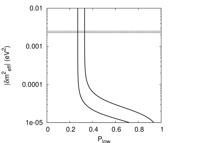
Figure 1: Correlation of $\delta m^{2}_{eff}$ for high-energy atmospheric and long-baseline neutrinos with the oscillation probability $P_{low}$ for low-energy solar neutrinos in the generalized direction-independent bicycle model (between the solid curves), found by varying the model parameter $a_{11}$. The left (right) solid curve assumes $E_{min}=8.0$ MeV (12 MeV) and $P_{min}=0.27~{}(0.33)$. The region between the horizontal dotted lines is consistent with atmospheric and long-baseline neutrino experiments.

The probability reaches the minimum at

$$E_{min}={1\over c}\left[a_{11}+b\right]\,,$$ (17)

which must occur in the energy region of the ⁸B solar neutrinos ($E_{min}\approx 10$ MeV), which fixes the magnitude of $c$ to be

$$|c|={1\over E_{min}}\left|a_{11}+b\right|={1.2~{}b\over E_{min}}\approx 2.0\times 10^{-19}\,.$$ (18)

Using Eq. (12) we may now calculate the value of the atmospheric $\delta m^{2}_{eff}$ inferred from solar neutrino data: $\delta m^{2}=a^{2}/c=2.2\times 10^{-5}$ eV², which is two orders of magnitude below the measured value.

One caveat for this calculation is that the low-energy solar oscillation probability is not measured precisely, and the model prediction may be adjusted by changing $a_{11}$. This in turn changes $c$ (via Eq. 18) and the predicted atmospheric $\delta m^{2}_{eff}$ (via Eq. 12). The relationship between $\delta m^{2}_{eff}$ and $P_{low}$ is shown in Fig. 1, where we have assumed 8 MeV $<E_{min}<$ 12 MeV and 0.27 $<P_{min}<$ 0.33.

For the range of $\delta m^{2}_{eff}$ allowed by experiment (shown by the horizontal dashed lines), the low-energy probability is approximately $0.30$, which is not consistent with $P_{low}\approx 0.57$ preferred by the solar data. In fact, any $\delta m^{2}_{eff}$ above $10^{-4}$ eV² gives a value for $P_{low}$ below 0.40. Therefore there is no acceptable value for $a_{11}$ that fits both the low-energy solar oscillation probability and $\delta m^{2}_{eff}$ for high-energy atmospheric and long-baseline neutrinos, and the generalized direction-independent bicycle model is excluded.

3 Other textures for $h_{eff}$

3.1 Classification of models

There are six possible $c$ coefficients in $h_{eff}$: three real diagonal coefficients and three complex off-diagonal coefficients (the remaining three off-diagonals are fixed by the hermiticity of $h_{eff}$). Therefore there are $2^{6}=64$ possible $c$ textures for $h_{eff}$. Since the high-energy behavior of $h_{eff}$ is determined by the $c$ coefficients, we classify the models by the number of nonzero $c$ there are in $h_{eff}$. Within each main class there are distinct subclasses which depend on the diagonal/off-diagonal structure; within each subclass there are textures that differ only by permutation of the flavor indices. In all there are 19 subclasses, which are listed in Table 1.

Table 1: A list of the 64 possible $c$ textures for $h_{eff}$. The number in the subclass name corresponds to the number of nonzero $c$, while the letters indicate a distinct diagonal/off-diagonal structure (up to flavor permutation), if applicable. A $D_{i}$ in the structure column indicates that a diagonal $c_{ii}$ is nonzero, while an $O_{jk}$ indicates that off-diagonal $c_{jk}$ is nonzero. Different latin indices in each case are distinct, e.g., in the structure $D_{i}O_{jk}$ the diagonal element does not share a row or column with the off-diagonal element, whereas for $D_{i}O_{ij}$ it does.

Number of	Subclass	Structure	Number of flavor
nonzero $c$			permutations
0	0	$-$	1
1	1A	$D_{i}$	3
	1B	$O_{ij}$	3
2	2A	$D_{i}D_{j}$	3
	2B	$D_{i}O_{ij}$	6
	2C	$D_{i}O_{jk}$	3
	2D	$O_{ij}O_{ik}$	3
3	3A	$D_{i}D_{j}D_{k}$	1
	3B	$D_{i}D_{j}O_{ij}$	3
	3C	$D_{i}D_{j}O_{ik}$	6
	3D	$D_{i}O_{ij}O_{ik}$	3
	3E	$D_{j}O_{ij}O_{ik}$	6
	3F	$O_{ij}O_{ik}O_{jk}$	1
4	4A	$D_{i}D_{j}D_{k}O_{ij}$	3
	4B	$D_{i}D_{j}O_{ij}O_{ik}$	6
	4C	$D_{i}D_{j}O_{ik}O_{jk}$	3
	4D	$D_{i}O_{ij}O_{ik}O_{jk}$	3
5	5A	$D_{i}D_{j}D_{k}O_{ij}O_{ik}$	3
	5B	$D_{i}D_{j}O_{ij}O_{ik}O_{jk}$	3
6	6	$D_{i}D_{j}D_{k}O_{ij}O_{ik}O_{jk}$	1

We note that we may subtract any quantity proportional to the identity from $h_{eff}$, since common phases in the neutrino equations of motion do not affect the oscillations. In this way a diagonal element may be removed or moved from one position to another. Then it is not hard to see that the following subclasses are strictly equivalent: 3A$\leftrightarrow$2A, 3C$\leftrightarrow$3B, 4A$\leftrightarrow$3B, 4C$\leftrightarrow$4B, 5A$\leftrightarrow$4B and 6$\leftrightarrow$5B.

3.2 Method for analyzing textures

Our analysis proceeds as follows. We assume that $|c_{ij}E|\gg|a_{k\ell}|$ for any $(i,j,k,\ell)$ for the high energies of atmospheric and long-baseline neutrinos. This assumption is justified since if any $a$ is similar in magnitude to the $cE$ at high energies, then at lower energies (such as for reactor neutrinos) the $a$ terms will dominate and the oscillation arguments will be energy-independent, contrary to the KamLAND data, which measured a spectral distortion (similarly, solar neutrinos would also not have an energy-dependent oscillation probability, as they must). Furthermore, for the sake of naturalness, we assume that the $c$ coefficients are all the same order of magnitude, and that likewise the $a$ coefficients are also the same order of magnitude.

Although for each texture the number of nonzero $c$ is determined, initially we place no restrictions on the $a$. We note that if all off-diagonal $c$ are nonzero, then by a redefinition of neutrino phases and adding a term proportional to the identity we may take all off-diagonal $c$ to be real and positive, except for one off-diagonal $c$ that is complex (which we take to be $c_{13}$ unless otherwise noted). If any off-diagonal $c$ is zero, the nonzero off-diagonal $c$ may all be taken as real and positive.

A key feature of the bicycle model was that even though the terms in the effective Hamiltonian were either proportional to energy or constant in energy, one eigenvalue difference was proportional to $E^{-1}$, which mimics the energy dependence of the oscillations of atmospheric and long-baseline neutrinos. Having an eigenvalue difference proportional to $E^{-1}$ means that if the eigenvalues are expanded in a power series in neutrino energy,

$$\lambda_{i}=\sum_{j=0}^{\infty}a_{ij}E^{1-j}\,,\qquad{\rm~{}for~{}}i=1,2,3\,$$ (19)

then two eigenvalues must be degenerate at leading order in $E$ (linear in $E$), and at the next order in energy ($E^{0}$, independent of energy). Therefore in our analysis of more general three-neutrino models with Lorentz invariance violation, we look for model parameters that satisfy these conditions. Since an $L/E$ dependence has been seen over many orders of magnitude in neutrino energy [16], it seems likely that this is the only way the Hamiltonian in Eq. (1) will be able to fit all atmospheric and long-baseline neutrino data.

For each texture we expand the eigenvalues of $h_{eff}$ in powers of $E$ (as in Eq. 19), where the leading $E^{1}$ behavior comes from the dominant $cE$ terms. Since we want $1/E$ behavior for at least one oscillation argument, we require that two of the eigenvalues be degenerate to order $E^{0}$, with the first nonzero difference occurring at order $E^{-1}$. In all cases this requirement puts constraints on the $c$ and $a$ coefficients. In our calculations we first find the eigenvalues to order $E^{1}$ and impose the constraint that two eigenvalues must be degenerate; then we find the eigenvalues of the simplified $h_{eff}$ to order $E^{0}$ and again impose the degeneracy condition. In this way the expressions for the eigenvalues to order $E^{-1}$ will be made as simple as possible at each stage of the calculation.

If the appropriate $1/E$ behavior can be achieved, the mixing angles are then calculated to determine if $\nu_{\mu}$’s have maximal mixing and $\nu_{e}$ small mixing for atmospheric and long-baseline neutrinos. If the model is still viable, the energy dependences of the oscillations of solar and KamLAND neutrinos are then checked for consistency.

At any time we are allowed to subtract a constant times the identity matrix from $h_{eff}$. Some cases may then be further simplified, or made equivalent to other cases (see below for specific examples). Rotations are also sometimes used to show that some cases are equivalent to others.

3.3 No $c$ parameters

In this case, Class 0, $h_{eff}$ has only $a$ terms and therefore is independent of energy. This clearly cannot produce $1/E$ behavior at high energy, so this category is immediately ruled out.

3.4 One $c$ parameter

3.4.1 Class 1A

This case has the structure

$$h_{eff}=\pmatrix{cE+a_{11}&a_{12}&a_{13}\cr a_{12}^{*}&a_{22}&a_{23}\cr a_{13}^{*}&a_{23}^{*}&a_{33}}\,,$$ (20)

where $c_{11}\equiv c$ may be taken as real and positive. The eigenvalues to order $E^{0}$ are then

$$\lambda_{1}=cE+a_{11}\,,\quad\lambda_{2},\lambda_{3}={1\over 2}\left[a_{22}+a_{33}\pm\sqrt{(a_{22}-a_{33})^{2}+4|a_{23}|^{2}}\right]\,.$$ (21)

The difference $\lambda_{2}-\lambda_{3}$ can only be made zero to order $E^{0}$ if $a_{22}=a_{33}$ and $|a_{23}|=0$. Then $a_{33}$ times the identity may be subtracted from $h_{eff}$; if $a_{11}-a_{33}$ is redefined as $a_{11}$, this case reduces to the generalized bicycle model described in Sec. 2, which is excluded by the combined data.

3.4.2 Class 1B

This case has the structure

$$h_{eff}=\pmatrix{a_{11}&cE+a_{12}&a_{13}\cr cE+a_{12}^{*}&a_{22}&a_{23}\cr a_{13}^{*}&a_{23}^{*}&a_{33}}\,,$$ (22)

where $c_{12}\equiv c$ may be taken as real and positive. The eigenvalues to order $E^{1}$ are then

$$\lambda_{1},\lambda_{2}=\pm|c|E\,,\quad\lambda_{3}=0\,.$$ (23)

Since these are all different at leading order, they cannot give an oscillation argument proportional to $E^{-1}$ at high energies, and this case is not allowed.

3.5 Two $c$ parameters

3.5.1 Class 2A

This case has the structure

$$h_{eff}=\pmatrix{c_{11}E+a_{11}&a_{12}&a_{13}\cr a_{12}^{*}&c_{22}E+a_{22}&a_{23}\cr a_{13}^{*}&a_{23}^{*}&a_{33}}\,,$$ (24)

where $c_{11}$ and $c_{22}$ are real. The eigenvalues at leading order are

$$\lambda_{1}=c_{11}E\,,\qquad\lambda_{2}=c_{22}E\,,\qquad\lambda_{3}=0\,,$$ (25)

so that we must have $c_{11}=c_{22}$ for degeneracy (having one of the $c_{ii}=0$ also works, but then it is in Class 1A instead of 2A). Now if $c_{11}E$ times the identity is subtracted from $h_{eff}$, this reduces to Class 1A, which is ruled out.

3.5.2 Class 2B

This case has the structure

$$h_{eff}=\pmatrix{c_{11}E+a_{11}&c_{12}E+a_{12}&a_{13}\cr c_{12}E+a_{12}^{*}&a_{22}&a_{23}\cr a_{13}^{*}&a_{23}^{*}&a_{33}}\,,$$ (26)

where $c_{11}$ and $c_{12}$ may be taken as real and positive. The eigenvalues at leading order are

$$\lambda_{1},\lambda_{2}={1\over 2}\left[c_{11}\pm\sqrt{c_{11}^{2}+4c_{12}^{2}}\right]E\,,\qquad\lambda_{3}=0\,.$$ (27)

Degeneracy requires (i) $\lambda_{1}=\lambda_{2}$, which is not possible for nonzero $c_{11}$ and $c_{12}$, or (ii) $\lambda_{3}=\lambda_{1}$ or $\lambda_{2}$, which is not possible for nonzero $c_{12}$. Therefore this case is not allowed.

3.5.3 Class 2C

This case has the structure

$$h_{eff}=\pmatrix{a_{11}&a_{12}&c_{13}E+a_{13}\cr a_{12}^{*}&c_{22}E&a_{23}\cr c_{13}E+a_{13}^{*}&a_{23}^{*}&a_{33}}\,,$$ (28)

where $c_{22}$ and $c_{13}$ may be taken as real and positive, and we have subtracted a term proportional to the identity so that $a_{22}=0$. The eigenvalues at leading order are

$$\lambda_{1},\lambda_{2}=\mp c_{13}E\,,\qquad\lambda_{3}=c_{22}E\,.$$ (29)

Degeneracy requires $c_{13}=c_{22}$. If we define $c_{22}=c_{13}\equiv c$, where $c$ is a positive real number; then the eigenvalues to order $E^{0}$ are

$$\lambda_{1}=-cE+{1\over 2}\left[a_{11}+a_{33}-2{\rm Re}(a_{13})\right]\,,\qquad\lambda_{2},\lambda_{3}=cE+{1\over 4}\left[x\pm\sqrt{x^{2}+8|y|^{2}}\right]\,,$$ (30)

where $x\equiv a_{11}+a_{33}+2{\rm Re}(a_{13})$ and $y\equiv a_{12}+a_{23}^{*}$. Degeneracy to order $E^{0}$ requires $x=0$ and $y=0$, which implies $a_{11}+a_{33}=-2{\rm Re}(a_{13})$ and $a_{12}=-a_{23}^{*}$. With these conditions the eigenvalues to order $E^{-1}$ are

$$\lambda_{1} = -cE+a_{11}+a_{33}-{1\over 2cE}(2|a_{23}|^{2}+|a_{13}|^{2}-a_{11}a_{33})\,,$$ (31)

$$\lambda_{2} = cE+{1\over 2cE}(2|a_{23}|^{2}+|a_{13}|^{2}-a_{11}a_{33})\,,\qquad\lambda_{3}=cE\,.$$ (32)

Clearly $\Delta_{32}=\lambda_{3}-\lambda_{2}$ has the correct energy dependence for atmospheric and long-baseline oscillations. The mixing matrix such that $U^{T}h_{eff}U$ is diagonal at leading order is given by

$$U=\pmatrix{-{1\over\sqrt{2}}&{1\over\sqrt{2}}\sin\theta&{1\over\sqrt{2}}\cos\theta\cr 0&\cos\theta&-\sin\theta\cr{1\over\sqrt{2}}&{1\over\sqrt{2}}\sin\theta&{1\over\sqrt{2}}\cos\theta}\,,$$ (33)

where $\sin\theta=|a_{11}+a_{13}|/\sqrt{2|a_{23}|^{2}+|a_{11}+a_{13}|^{2}}$ and the oscillation probabilities are approximately given by

$$P(\nu_{\mu}\to\nu_{\mu}) = 1-\sin^{2}2\theta\sin^{2}\left({1\over 2}\Delta_{32}L\right)\,,$$ (34)

$$P(\nu_{\mu}\to\nu_{e}) = P(\nu_{\mu}\to\nu_{\tau})={1\over 2}\sin^{2}2\theta\sin^{2}\left({1\over 2}\Delta_{32}L\right)\,.$$ (35)

Therefore maximal mixing for $\nu_{\mu}$ is possible with $\delta m^{2}_{eff}=2E\Delta_{23}=(2|a_{23}|^{2}+|a_{13}|^{2}-a_{11}a_{33})/c$, but $\nu_{\mu}$ oscillates equally to $\nu_{e}$ and $\nu_{\tau}$, which is excluded by atmospheric neutrino experiments. Hence this case is not allowed.

3.5.4 Class 2D

This case has the structure

$$h_{eff}=\pmatrix{a_{11}&c_{12}E+a_{12}&c_{13}E+a_{13}\cr c_{12}E+a_{12}^{*}&a_{22}&a_{23}\cr c_{13}E+a_{13}^{*}&a_{23}^{*}&a_{33}}\,,$$ (36)

where $c_{12}$ and $c_{13}$ may be taken as real and positive. If a rotation is applied to the $\mu-\tau$ sector, then $c_{13}$ may be rotated away into $c_{12}$, which reduces this case to Class 1B, which is not allowed.

3.6 Three $c$ parameters

3.6.1 Class 3A

This subclass has nonzero $c$ in each diagonal term and no off-diagonal $c$. By subtracting off $c_{33}E$ times the identity, this case reduces to Class 2A, which is not allowed.

3.6.2 Class 3B

This case has the structure

$$h_{eff}=\pmatrix{c_{11}E+a_{11}&a_{12}&c_{13}E+a_{13}\cr a_{12}^{*}&0&a_{23}\cr c_{13}E+a_{13}^{*}&a_{23}^{*}&c_{33}E+a_{33}}\,,$$ (37)

where $c_{11}$, $c_{33}$ and $c_{13}$ may be taken as real and $a_{22}$ has been set to zero by a subtraction proportional to the identity. The eigenvalues at leading order are

$$\lambda_{1},\lambda_{2}={1\over 2}\left[c_{11}+c_{33}\pm\sqrt{(c_{11}-c_{33})^{2}+4c_{13}^{2}}\right]E\,,\qquad\lambda_{3}=0\,.$$ (38)

There are two possible ways to have a degeneracy. First, if $\lambda_{1}=\lambda_{2}$, then we must have $c_{11}=c_{33}$ and $c_{13}=0$. However, if $c_{11}E$ times the identity is then subtracted from $h_{eff}$, this possibility reduces to Class 1A. Second, we can have $\lambda_{2}=0$, so that it is degenerate with $\lambda_{3}$. There is a family of such solutions with $c_{33}=r^{2}c_{11}$ and $c_{13}=rc_{11}$, where $r$ may be taken as a positive real number. If we define $c_{11}\equiv c$, then to order $E^{0}$ the eigenvalues are

$$\lambda_{1}=(1+r^{2})cE+a_{11}+a_{33}-x\,,\qquad\lambda_{2},\lambda_{3}={1\over 2}\left[x\pm\sqrt{x^{2}+4y}\right]\,,$$ (39)

where $x=[a_{33}+r^{2}a_{11}-2r{\rm Re}(a_{13})]/(1+r^{2})$ and $y=|ra_{12}-a_{23}^{*}|^{2}/(1+r^{2})$. Degeneracy is only possible if $x=0$ and $y=0$, which requires $a_{33}+r^{2}a_{11}=2r{\rm Re}(a_{13})$ and $a_{23}=ra_{12}^{*}$, respectively. The eigenvalues to order $E^{-1}$ are then

$$\lambda_{1} = (1+r^{2})cE+a_{11}+a_{33}+{|a_{13}|^{2}+(1+r^{2})|a_{12}|^{2}-a_{11}a_{33}\over(1+r^{2})cE}\,,$$ (40)

$$\lambda_{2} = -{|a_{13}|^{2}+(1+r^{2})|a_{12}|^{2}-a_{11}a_{33}\over(1+r^{2})cE}\,,\qquad\lambda_{3}=0\,.$$ (41)

Thus $\Delta_{32}$ has the correct energy dependence, and gives

$$\delta m^{2}_{eff}=2E\Delta_{32}=2{|a_{13}|^{2}+(1+r^{2})|a_{12}|^{2}-a_{11}a_{33}\over(1+r^{2})c}=2{|ra_{11}-a_{13}|^{2}+(1+r^{2})|a_{12}|^{2}\over c(1+r^{2})}\,,$$ (42)

for atmospheric and long-baseline neutrinos. We note that $\lambda_{3}=0$ is an exact result given the degeneracy conditions, true even when $E$ is not large.

To leading order the mixing matrix that diagonalizes $h_{eff}$ via $U^{T}h_{eff}U$ is

$$U=\pmatrix{\cos\phi&\sin\phi\cos\theta&-\sin\phi\sin\theta\cr 0&\sin\theta&\cos\theta\cr\sin\phi&-\cos\phi\cos\theta&\cos\phi\sin\theta}\,,$$ (43)

where $\sin\phi\equiv r/\sqrt{1+r^{2}}$ and $\tan\theta\equiv\sqrt{1+r^{2}}|a_{12}|/|ra_{11}-a_{13}|$. This mixing gives the oscillation probabilities

$$P(\nu_{\mu}\to\nu_{\mu}) = 1-\sin^{2}2\theta\sin^{2}\left(\Delta_{32}{L\over 2}\right)\,,$$ (44)

$$P(\nu_{\mu}\to\nu_{e}) = \sin^{2}\phi\sin^{2}2\theta\sin^{2}\left(\Delta_{32}{L\over 2}\right)\,,$$ (45)

$$P(\nu_{e}\to\nu_{e}) = 1-\cos^{2}\theta\sin^{2}2\phi\sin^{2}\left(\Delta_{21}{L\over 2}\right)-\sin^{2}\theta\sin^{2}2\phi\sin^{2}\left(\Delta_{31}{L\over 2}\right)$$ (46)

$$\phantom{1-}-\sin^{4}\phi\sin^{2}2\theta\sin^{2}\left(\Delta_{32}{L\over 2}\right)\,.$$

Maximal $\nu_{\mu}$ oscillations are possible for $\theta\simeq\pi/4$, which imposes the condition $\sqrt{1+r^{2}}|a_{12}|\simeq|ra_{11}-a_{13}|$.

Oscillations of $\nu_{e}$ at high energies must be small due to the limit on $\nu_{\mu}\to\nu_{e}$ from K2K [17] and MINOS [18]. For K2K and MINOS the oscillation amplitude for $P(\nu_{\mu}\to\nu_{e})$, $\sin^{2}\phi\sin^{2}2\theta$, has an upper bound of about 0.14, which implies $r<0.43$ for $\theta\simeq\pi/4$. The T2K experiment sees evidence for $\nu_{\mu}\to\nu_{e}$ at the $2.5\sigma$ level [19]; their allowed regions are consistent with this bound.

We note that the conditions $c_{33}=r^{2}c_{11}$ and $c_{13}=rc_{11}$ require fine tuning. If these conditions are not exact, they introduce small corrections, which may be absorbed into the $a$ terms, e.g., $a_{ij}\to a_{ij}+\delta c_{ij}E$, where $\delta c_{ij}$ represents the deviation from the exact degeneracy condition. This effectively introduces an $E$ dependence into $\delta m^{2}_{eff}$, contrary to the atmospheric and long-baseline data.

For solar or reactor neutrinos the large energy limit does not apply. Then the eigenvalues are

$$\lambda_{1},\lambda_{2} = {1\over 2}\left[cE(1+r^{2})+a_{11}+a_{33}\pm\sqrt{[cE(1+r^{2})+a_{11}+a_{33}]^{2}+2\delta m^{2}_{eff}c(1+r^{2})}\right]$$

$$\qquad\lambda_{3} = 0\,.$$ (47)

where $\delta m^{2}_{eff}$ is from Eq. (42), and it can be shown that the matrix that diagonalizes $h_{eff}$ is

$$U=\pmatrix{\cos\phi\cos\xi+\sin\phi\cos\theta\sin\xi e^{-i\delta}&-\cos\phi\sin\xi+\sin\phi\cos\theta\cos\xi e^{-i\delta}&-\sin\phi\sin\theta\cr\sin\theta\sin\xi&\sin\theta\cos\xi&\cos\theta e^{i\delta}\cr\sin\phi\cos\xi-\cos\phi\cos\theta\sin\xi e^{-i\delta}&-\sin\phi\sin\xi-\cos\phi\cos\theta\cos\xi e^{-i\delta}&\cos\phi\sin\theta}\,,$$ (48)

where $\phi$ and $\theta$ are defined as above, $\tan\xi=|ra_{11}-a_{13}|/(\lambda_{1}\cos\theta)$ and $\delta={\rm~{}arg}(ra_{11}-a_{13})$. Note that in the large energy limit $\lambda_{1}$ is large, $\xi\to 0$, and Eq. (48) reduces to Eq. (43). Also, since none of the mixings are zero, $CP$ violation is possible.

We checked KamLAND phenomenology first. Since we have obtained several conditions from fitting the atmospheric and long-baseline neutrinos, using these conditions we can vary $a_{11}$, $a_{13}$ and $r$ to fit the KamLAND data [20]. Other parameters in the effective Hamiltonian will be determined by these three parameters. Scanning the $a_{11}$, $a_{13}$ and $r$ parameter space, we find the following parameter values yield reasonable agreement with the KamLAND data (see Fig. 2):

$$a_{11}=-8.7\times 10^{-11}{\rm~{}eV}\,,\ \ \ \ \ a_{13}=-9.5\times 10^{-11}{\rm~{}eV}\,,\ \ \ \ \ r=0.1\,.$$ (49)

However, the fit is not as good as the standard oscillation scenario with neutrino mass.

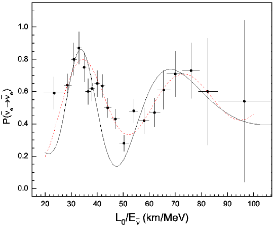
Figure 2: The best fit to the KamLAND data for Class 3B (solid lines) and the standard oscillation scenario with neutrino masses (dashed lines). For the model parameters see Eq. (49).

Next we use these parameter values to check the solar phenomenology. Since the operator for $a$ breaks $CPT$, we reverse the sign of $a$ when we apply these parameter values to the solar neutrinos. However, the prediction does not agree with the solar data at high energies given the upper bound on $r$ from above (see Fig. 3).

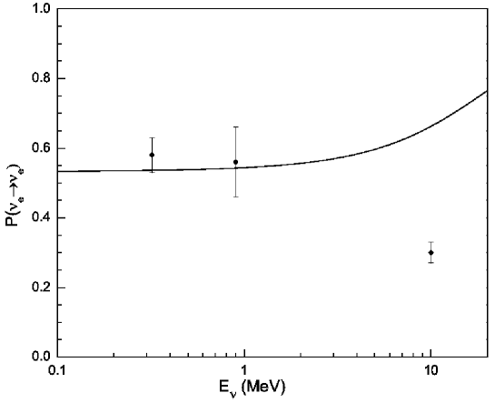
Figure 3: The prediction of Class 3B for the oscillation probability of solar neutrinos using the parameter values obtained from fitting KamLAND data [20]. The solar data points are from an update of the analysis in Ref. [21].

We also searched the $a_{11}$, $a_{13}$ and $r$ parameter space to fit the solar data separately. The best fit still can not yield reasonable agreement with the solar data at high energies for $r<0.43$ (see Fig. 4). If we do not impose the constraint on $r$, the fit to the solar data is improved at high energies (see Fig. 5). However, we cannot simultaneously fit the KamLAND and solar data even with larger $r$. We found that we also need $|a_{11}|$ to become larger in order to fit the solar data, but larger $|a_{11}|$ yields fast oscillations for KamLAND data with averaged probabilities around $1/2$.

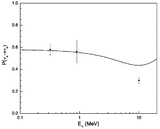
Figure 4: Best fit prediction for survival probability of $\nu_{e}$ for solar neutrinos for Class 3B, assuming $r<0.43$. The model parameters for the best fit are $a_{11}=-1.0\times 10^{-10}{\rm~{}eV},a_{13}=7.3\times 10^{-11}{\rm~{}eV}$ and $r=0.4$.

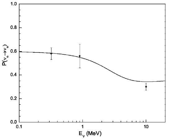
Figure 5: Best fit prediction for survival probability of $\nu_{e}$ for solar neutrinos alone in Class 3B, assuming $r>0.43$. The model parameters are $a_{11}=-5.0\times 10^{-10}{\rm~{}eV},a_{13}=-3.1\times 10^{-11}$ eV and $r=1.0$.

3.6.3 Class 3C

This case has the structure

$$h_{eff}=\pmatrix{c_{11}E+a_{11}&a_{12}&c_{13}E+a_{13}\cr a_{12}^{*}&c_{22}E+a_{22}&a_{23}\cr c_{13}E+a_{13}^{*}&a_{23}^{*}&a_{33}}\,,$$ (53)

where $c_{11}$ and $c_{22}$ are real and $c_{13}$ may be taken as real and positive. By subtracting $c_{22}$ times the identity, this case reduces to Class 3B, which was described in the previous section.

3.6.4 Class 3D

This case has the structure

$$h_{eff}=\pmatrix{c_{11}E+a_{11}&c_{12}E+a_{12}&c_{13}E+a_{13}\cr c_{12}E+a_{12}^{*}&a_{22}&a_{23}\cr c_{13}E+a_{13}^{*}&a_{23}^{*}&a_{33}}\,,$$ (54)

where $c_{11}$, $c_{12}$ and $c_{13}$ may be taken as real and positive. If a rotation is applied to the $\mu-\tau$ sector, then $c_{13}$ may be rotated away, which reduces this case to Class 2B, which is not allowed.

3.6.5 Class 3E

This case has the structure

$$h_{eff}=\pmatrix{c_{11}E+a_{11}&c_{12}E+a_{12}&a_{13}\cr c_{12}E+a_{12}^{*}&a_{22}&c_{23}E+a_{23}\cr a_{13}^{*}&c_{23}E+a_{23}^{*}&a_{33}}\,,$$ (55)

where $c_{11}$, $c_{12}$ and $c_{23}$ may be taken as real and positive. This is the first case that cannot be simply reduced to a previous case, and which requires solving a nontrivial cubic equation to determine the eigenvalues at leading order. The eigenvalue equation for $h_{eff}/E$ at leading order is

$$\lambda^{3}-c_{11}\lambda^{2}-(c_{12}^{2}+c_{23}^{2})\lambda+c_{11}c_{23}^{2}=0\,.$$ (56)

For a cubic equation of the form $\lambda^{3}+a\lambda^{2}+b\lambda+c=0$, if we define $q=a^{2}-3b$ and $r=2a^{3}-9ab+27c$, then for three real roots the cubic discriminant $f\equiv 4q^{3}-r^{2}$ must be nonnegative, with $f=0$ when two of the roots are equal. Since the effective Hamiltonian is hermitian, the eigenvalues must be real, so $f\geq 0$. Therefore, if there is a degeneracy, not only must $f=0$, it must be a global minimum of $f$, i.e., we can search for degeneracies by finding the minima of $f$.

For this case we have

$$q=c_{11}^{2}+3(c_{12}^{2}+c_{23}^{2})\,,\qquad r=c_{11}(-2c_{11}^{2}+18c_{23}^{2}-9c_{12}^{2})\,,$$ (57)

and the discriminant is

$$f=4(c_{11}^{2}+3c_{12}+3c_{23}^{2})^{3}-c_{11}^{2}(2c_{11}^{2}+9c_{12}^{2}-18c_{23}^{2})^{2}\,.$$ (58)

Then,

$$0={\partial f\over\partial c_{12}}=108c_{12}\left[6c_{12}^{4}+6c_{23}^{4}+c_{11}^{2}c_{12}^{2}+10c_{11}^{2}+12c_{12}^{2}c_{23}^{2}\right]\,,$$ (59)

requires at least that $c_{12}=0$, which reduces this case to Class 2C, which is not allowed.

3.6.6 Class 3F

This case has the structure

$$h_{eff}=\pmatrix{a_{11}&c_{12}E+a_{12}&c_{13}E+a_{13}\cr c_{12}E+a_{12}^{*}&a_{22}&c_{23}E+a_{23}\cr c_{13}^{*}E+a_{13}^{*}&c_{23}E+a_{23}^{*}&0}\,,$$ (60)

where $c_{12}$ and $c_{23}$ may be taken as real and positive, $c_{13}$ is complex and $a_{33}$ has been set equal to zero. This case also requires solving a nontrivial cubic equation to find the eigenvalues at leading order; with

$$q=3(c_{12}^{2}+c_{13}^{2}+c_{23}^{2})\,,\qquad r=-54c_{12}c_{23}|c_{13}|c_{\delta}\,,$$ (61)

where $c_{\delta}=\cos\delta$ and $\delta$ is the phase of $c_{13}$. Searching for a minimum of $f=4q^{3}-r^{2}$:

$$0={\partial f\over\partial c_{12}} = 72c_{12}q^{2}+108r|c_{13}|c_{23}c_{\delta}\,,$$ (62)

$$0={\partial f\over\partial c_{13}} = 72|c_{13}|q^{2}+108rc_{12}c_{23}c_{\delta}\,,$$ (63)

$$0={\partial f\over\partial c_{23}} = 72c_{23}q^{2}+108rc_{12}|c_{13}|c_{\delta}\,,$$ (64)

$$0={\partial f\over\partial\delta} = -108rc_{12}|c_{13}|c_{23}\sin\delta\,.$$ (65)

The quantity $q$ is explicitly nonzero; if $r$ was zero then Eqs. (62)-(64) would imply that $c_{12}$, $c_{13}$ and $c_{23}$ would all have to be zero, which is not possible for this case, so $r\neq 0$. Then the last equation implies $\sin\delta=0$, or $\delta=0$ or $\pi$. Thus $c_{\delta}=\pm 1$, i.e., $c_{13}$ is real, but it might differ by a sign from $c_{12}$ and $c_{23}$; we use $c_{\delta}$ to denote this possible sign difference and henceforth take $c_{13}$ as real and positive.

It is not hard to show that $c_{12}=c_{13}=c_{23}$ is required for a minimum of $f$ and that this condition gives $f=0$. Therefore degeneracy requires $c_{12}=c_{13}=c_{23}\equiv c$ with $c_{\delta}=\pm 1$. Then the eigenvalues to order $E^{0}$ are

$$\lambda_{1}=2cEc_{\delta}+a_{11}+a_{22}-x\,,\qquad\lambda_{2},\lambda_{3}=-cEc_{\delta}+{1\over 2}\left[x\mp\sqrt{x^{2}-4y}\right]\,,$$ (66)

where

$$x = {2\over 3}\left[(a_{11}+a_{22})-{\rm Re}(a_{13})-c_{\delta}{\rm Re}(a_{12}+a_{23})\right],,$$ (67)

$$y = {1\over 3}\left[a_{11}a_{22}-|a_{12}|^{2}-|a_{13}|^{2}-|a_{23}|^{2}+2{\rm Re}(a_{12}a_{23}-a_{22}a_{13})\right.$$ (68)

$$\phantom{~{}{1\over 3}[}+\left.2c_{\delta}{\rm Re}(a_{12}a_{13}^{*}+a_{23}a_{13}^{*}-a_{11}a_{23})\right]\,.$$

Thus degeneracy requires that the quadratic discriminant $g=x^{2}-4y$ be zero. Since the eigenvalues are real, we know $g\geq 0$, and degeneracy can only occur at a minimum of $g$. It can be shown that $g$ has a minimum at zero for $a_{11}=a_{22}={\rm Re}(a_{12})={\rm Re}(a_{13})={\rm Re}(a_{23})=0$ and ${\rm Im}(a_{13})=c_{\delta}{\rm Im}(a_{12}+a_{23})$. Then

$$h_{eff}=\pmatrix{0&cE+ia_{12}&c_{\delta}[cE+i(a_{12}+a_{23})]\cr cE-ia_{12}&0&cE+ia_{23}\cr c_{\delta}[cE-i(a_{12}+a_{23})]&cE-ia_{23}&0}\,,$$ (69)

where the $a_{ij}$ are now defined as real. The eigenvalues of this matrix to order $E^{-1}$ are

$$\lambda_{1}=2c_{\delta}cE+{2c_{\delta}\over 3cE}(a_{12}^{2}+a_{23}^{2}+a_{12}a_{23})\,,\qquad\lambda_{2}=-c_{\delta}cE\,,\qquad\lambda_{3}=-c_{\delta}cE-{2c_{\delta}\over 3cE}(a_{12}^{2}+a_{23}^{2}+a_{12}a_{23})\,,$$ (70)

and the mixing matrix that diagonalizes $h_{eff}$ is

$$U=\pmatrix{{1\over\sqrt{3}}&{1\over N}a_{23}&-{c_{\delta}\over\sqrt{3}N}(a_{23}+2a_{12})\cr{c_{\delta}\over\sqrt{3}}&-{c_{\delta}\over N}(a_{12}+a_{23})&{1\over\sqrt{3}N}(a_{12}-a_{23})\cr{1\over\sqrt{3}}&{1\over N}a_{12}&{c_{\delta}\over\sqrt{3}N}(a_{12}+2a_{23})}\,,$$ (71)

where $N=\sqrt{2(a_{12}^{2}+a_{23}^{2}+a_{12}a_{23})}$ is a normalization factor.

At high energies for the fast oscillation $\Delta_{31}\simeq\Delta_{21}\simeq-3c_{\delta}cE$, all off-diagonal oscillation probabilities have the same approximate form:

$$P(\nu_{\alpha}\rightarrow\nu_{\beta})=\frac{4}{9}\sin^{2}\left(\frac{3cEL}{2}\right)\,.$$ (72)

For this oscillation amplitude, 4/9, the NuTeV limit on $\nu_{\mu}\to\nu_{e}$ [22] gives a 90% C.L. upper bound on $\delta m_{eff}^{2}$ of 3.6 eV². Since we have $\delta m_{eff}^{2}=6cE^{2}$ in this case and the average neutrino energy was 74 GeV, the experiment imposes the upper bound $c\leq 1.1\times 10^{-22}$. On the other hand, in order for the expansion in powers of $E$ to be valid, we need $N/(cE)\ll 1$ for $E\mathrel{\raise 1.29167pt\hbox{$>$\kern-7.5pt\lower 4.30554pt\hbox{$\sim$}}}100$ MeV, which leads to the lower bound $c>4\times 10^{-17}$. Therefore the structure required for the $1/E$ behavior at high energy is inconsistent with accelerator bounds. Since all flavors have the same survival probability in the fast oscillation, the result is the same even if a different permutation of flavors is taken.

Furthermore, for the $\Delta_{23}$ oscillations in atmospheric and long-baseline neutrinos, all three flavors have the probability

$$P(\nu_{\alpha}\rightarrow\nu_{\alpha})=\frac{5}{9}-4{|U_{\alpha 2}|}^{2}\left(\frac{2}{3}-{|U_{\alpha 2}|}^{2}\right)\sin^{2}\left(\frac{\Delta_{23}L}{2}\right)\,.$$ (73)

This implies that all flavors of downward atmospheric neutrinos would be suppressed by a factor of 5/9, which is contrary to the data. Therefore this case is excluded.

3.7 Four $c$ parameters

3.7.1 Class 4A

This case has three nonzero diagonal and one nonzero diagonal $c$. By subtracting a piece proportional to the identity, this case may be reduced to either Class 3B or 3C.

3.7.2 Class 4B

This case has the structure

$$h_{eff}=\pmatrix{c_{11}E+a_{11}&c_{12}E+a_{12}&c_{13}E+a_{13}\cr c_{12}E+a_{12}^{*}&c_{22}E+a_{22}&a_{23}\cr c_{13}E+a_{13}^{*}&a_{23}^{*}&a_{33}}\,,$$ (74)

where $c_{11}$ and $c_{22}$ are real and $c_{12}$ and $c_{13}$ may be taken as positive. The eigenvalue equation for $h_{eff}/E$ at leading order is

$$\lambda^{3}-(c_{11}+c_{22})\lambda^{2}+(c_{11}c_{22}-c_{12}^{2}-c_{23}^{2})\lambda+c_{22}c_{13}^{2}=0\,.$$ (75)

This case has cubic discriminant

$$f=4q^{3}-r^{2}\,,$$ (76)

where

$$q \equiv c_{11}^{2}+c_{22}^{2}-c_{11}c_{22}+3c_{12}^{2}+3c_{13}^{2}\,,$$ (77)

$$r \equiv -2c_{11}^{3}+3c_{11}^{2}c_{22}+3c_{11}c_{22}^{2}-2c_{22}^{3}-9c_{11}(c_{12}^{2}+c_{13}^{2})+9c_{22}(2c_{13}^{2}-c_{12}^{2})\,,$$ (78)

The minimum conditions are

$$0 = {\partial f\over\partial c_{11}}=12(2c_{11}-c_{22})q^{2}-2r\left[-6c_{11}^{2}+6c_{11}c_{22}+3c_{22}^{2}-9(c_{12}^{2}+c_{13}^{2})\right]\,,$$ (79)

$$0 = {\partial f\over\partial c_{22}}=12(2c_{22}-c_{11})q^{2}-2r\left[-6c_{22}^{2}+6c_{22}c_{11}+3c_{11}^{2}+9(2c_{13}^{2}-c_{12}^{2})\right]\,,$$ (80)

$$0 = {\partial f\over\partial c_{12}}=72c_{12}q^{2}+36rc_{12}(c_{11}+c_{22})\,,$$ (81)

$$0 = {\partial f\over\partial c_{13}}=72c_{13}q^{2}-36rc_{13}(2c_{22}-c_{11})\,.$$ (82)

Clearly $q>0$ if none of the $c_{ij}$ are zero. If $r=0$, then Eqs. (81) and (82) would imply $c_{12}=c_{13}=0$, which is not Class 4B; therefore $r\neq 0$. Then Eqs. (81) and (82) imply

$$-{1\over c_{11}+c_{22}}={r\over q^{2}}={1\over 2c_{22}-c_{11}}\,,$$ (83)

which implies $c_{22}=0$. This case then reduces to Class 3D, which is not allowed.

3.7.3 Class 4C

This case has the structure

$$h_{eff}=\pmatrix{c_{11}E+a_{11}&a_{12}&c_{13}E+a_{13}\cr a_{12}^{*}&c_{22}E+a_{22}&c_{23}E+a_{23}\cr c_{13}E+a_{13}^{*}&c_{23}E+a_{23}^{*}&a_{33}}\,,$$ (84)

where $c_{11}$ and $c_{22}$ are real and $c_{13}$ and $c_{23}$ may be taken as real and positive. By subtracting $c_{11}$ times the identity this case may be reduced to Class 4B, which is not allowed.

3.7.4 Class 4D

This case has the structure

$$h_{eff}=\pmatrix{c_{11}E+a_{11}&c_{12}E+a_{12}&c_{13}E+a_{13}\cr c_{12}E+a_{12}^{*}&a_{22}&c_{23}E+a_{23}\cr c_{13}^{*}E+a_{13}^{*}&c_{23}E+a_{23}^{*}&a_{33}}\,,$$ (85)

where $c_{11}$, $c_{12}$ and $c_{23}$ may be taken as real, and $c_{13}$ is complex. The eigenvalue equation for $h_{eff}/E$ at leading order is

$$\lambda^{3}-c_{11}\lambda^{2}+-(c_{12}^{2}+c_{13}^{2}+c_{23}^{2})\lambda+c_{11}c_{23}^{2}-2c_{12}c_{13}c_{23}c_{\delta}=0\,,$$ (86)

where $c_{\delta}\equiv\cos\delta$, $c_{13}\to c_{13}e^{i\delta}$ and $c_{13}$ is now taken as real and positive. This case has

$$q \equiv c_{11}^{2}+3(c_{12}^{2}+c_{13}^{2}+c_{23}^{2})\,,$$ (87)

$$r \equiv -2c_{11}^{3}+9c_{11}(2c_{23}^{2}-c_{12}^{2}-c_{13}^{2})-54c_{12}c_{13}c_{23}c_{\delta}\,,$$ (88)

where the discriminant is $f=4q^{3}-r^{2}$. The minimum conditions are

$$0 = {\partial f\over\partial c_{11}}=24c_{11}q^{2}-2r\left[-6c_{11}^{2}+9(2c_{23}^{2}-c_{12}^{2}-c_{13}^{2})\right]\,,$$ (89)

$$0 = {\partial f\over\partial c_{12}}=72c_{12}q^{2}+36r(c_{11}c_{12}+3c_{13}c_{23}c_{\delta})\,,$$ (90)

$$0 = {\partial f\over\partial c_{13}}=72c_{13}q^{2}+36r(c_{11}c_{13}+3c_{12}c_{23}c_{\delta})\,,$$ (91)

$$0 = {\partial f\over\partial c_{23}}=72c_{23}q^{2}-36r(2c_{11}c_{23}-3c_{12}c_{13}c_{\delta})\,,$$ (92)

$$0 = {\partial f\over\partial\delta}=-108rc_{12}c_{13}c_{23}\sin\delta\,.$$ (93)

Clearly $q>0$ if none of the $c$ are zero. If $r=0$, then Eqs. (90)-(92) would imply $c_{12}=c_{13}=c_{23}=0$, which is not Class 4D; therefore $r\neq 0$. Thus Eq. (93) implies $\sin\delta=0$, or $c_{\delta}=\pm 1$; therefore the off-diagonal elements are real.

By combining Eqs. (90) and (91), we find $c_{12}=c_{13}$, and by combining Eqs. (90) and (92), we find $c_{12}^{2}=c_{23}^{2}+c_{11}c_{23}c_{\delta}$. Then $q=(c_{11}+3c_{\delta}c_{23})^{2}$ and $r=-2(c_{11}+3c_{\delta}c_{23})^{3}$. Clearly then $f=0$, and the conditions for degeneracy at leading order are

$$c_{12}=c_{13}\,,\qquad c_{12}^{2}=c_{23}^{2}+c_{\delta}c_{11}c_{23}\,.$$ (94)

Thus there is a two-parameter set of degeneracies at leading order for this texture; at leading order $h_{eff}$ has the form

$$h_{eff}=\pmatrix{c_{11}&S&Sc_{\delta}\cr S&0&c_{23}\cr Sc_{\delta}&c_{23}&0}E\,,$$ (95)

where $S\equiv\sqrt{c_{23}(c_{23}+c_{\delta}c_{11})}$. By applying the rotation

$$V=\pmatrix{1&0&0\cr 0&{1\over\sqrt{2}}&{1\over\sqrt{2}}c_{\delta}\cr 0&-{1\over\sqrt{2}}c_{\delta}&{1\over\sqrt{2}}}\,,$$ (96)

and adding a term $c_{\delta}c_{23}E$ times the identity, at leading order the new Hamiltonian is

$$h_{eff}^{\prime}=V^{T}h_{eff}V=\pmatrix{c_{11}+c_{\delta}c_{23}&0&\sqrt{2}Sc_{\delta}\cr 0&0&0\cr\sqrt{2}Sc_{\delta}&0&2c_{\delta}c_{23}}E\,.$$ (97)

Equation (97) has the form of Class 3B with $r=\sqrt{2c_{23}/(c_{23}+c_{\delta}c_{11})}$. The matrix that diagonalizes the original $h_{eff}$ is therefore $U^{\prime}=VU$, or

$$U^{\prime}=\frac{1}{\sqrt{2}}\pmatrix{\sqrt{2}\cos\phi&\sqrt{2}\sin\phi\cos\theta&-\sqrt{2}\sin\phi\sin\theta\cr c_{\delta}\sin\phi&\sin\theta-c_{\delta}\cos\phi\cos\theta&\cos\theta+c_{\delta}\cos\phi\sin\theta\cr\cos\phi&-c_{\delta}\sin\theta-\cos\phi\cos\theta&-c_{\delta}\cos\theta+\cos\phi\sin\theta}\,,$$ (98)

where $U$ is from Eq. (43). The oscillation probabilities are

$$P(\nu_{\mu}\rightarrow\nu_{\mu}) = 1-\left(\sin\theta-\cos\phi c_{\delta}\cos\theta\right)^{2}\left(\cos\theta+\cos\phi c_{\delta}\sin\theta\right)^{2}\sin^{2}\left(\Delta_{23}\frac{L}{2}\right)$$ (99)

$$-\sin^{2}\phi\left(\sin\theta-c_{\delta}\cos\phi\cos\theta\right)^{2}\sin^{2}\left(\Delta_{12}\frac{L}{2}\right)$$

$$-\sin^{2}\phi\left(\cos\theta-c_{\delta}\cos\phi\sin\theta\right)^{2}\sin^{2}\left(\Delta_{13}\frac{L}{2}\right)\,,$$

$$P(\nu_{\mu}\rightarrow\nu_{e}) = \sin^{2}\phi\sin 2\theta(\sin^{2}\phi\sin\theta\cos\theta-c_{\delta}\cos\phi\cos 2\theta)\sin^{2}\left(\Delta_{23}\frac{L}{2}\right)$$ (100)

$$-c_{\delta}\sin\phi\sin 2\phi(\sin\theta\cos\theta-c_{\delta}\cos\phi\cos^{2}\theta)\sin^{2}\left(\Delta_{12}\frac{L}{2}\right)$$

$$+c_{\delta}\sin\phi\sin 2\phi(\sin\theta\cos\theta+c_{\delta}\cos\phi\sin^{2}\theta)\sin^{2}\left(\Delta_{13}\frac{L}{2}\right)\,,$$

$$P(\nu_{e}\rightarrow\nu_{e}) = 1-\sin^{4}\phi\sin^{2}2\theta\sin^{2}\left(\Delta_{23}\frac{L}{2}\right)-\sin^{2}2\phi\cos^{2}\theta\sin^{2}\left(\Delta_{12}\frac{L}{2}\right)$$ (101)

$$-\sin^{2}2\phi\sin^{2}\theta\sin^{2}\left(\Delta_{13}\frac{L}{2}\right)\,.$$

In order to compare with the atmospheric and long-baseline neutrinos data, for large E, we should have $\Delta_{12}L,\Delta_{13}L\gg\Delta_{23}L\sim 1$. Then the oscillation probabilities are

$$P(\nu_{\mu}\rightarrow\nu_{\mu}) = 1-\left(\sin\theta-c_{\delta}\cos\phi\cos\theta\right)^{2}\left(\cos\theta+c_{\delta}\cos\phi\sin\theta\right)^{2}\sin^{2}\left(\Delta_{23}\frac{L}{2}\right)$$ (102)

$$-\frac{1}{2}\sin^{2}\phi(1+\cos^{2}\phi)\,,$$

$$P(\nu_{\mu}\rightarrow\nu_{e}) = \sin^{2}\phi\sin 2\theta(\sin^{2}\phi\sin\theta\cos\theta-c_{\delta}\cos\phi\cos 2\theta)\sin^{2}\left(\Delta_{23}\frac{L}{2}\right)+\frac{1}{4}\sin^{2}2\phi\,.$$ (103)

Maximal $\nu_{e}$ oscillations requires

$$1 \simeq \left(\sin\theta-c_{\delta}\cos\phi\cos\theta\right)^{2}\left(\cos\theta+c_{\delta}\cos\phi\sin\theta\right)^{2}$$ (104)

$$= 1-\sin^{2}\phi-(\cos^{2}\phi+\frac{1}{2}c_{\delta}\cos\phi-\frac{1}{4}\sin^{4}\phi)\sin^{2}2\theta$$

If $\phi$ is small and $\sin 2\theta\simeq 0$, the probabilities are appropriate for the atmospheric and long-baseline neutrinos. Since $\sin\phi\equiv r/\sqrt{1+r^{2}}$ and $\tan\theta\equiv\sqrt{1+r^{2}}|a_{12}|/|ra_{11}-a_{13}|$, this imposes the conditions: (i) $r\simeq 0$ and $a_{12}\simeq 0$, or (ii) $r\simeq 0$ and $ra_{11}\simeq a_{13}$.

Since this case is equivalent to Class 3B after a rotation in the $\nu_{\mu}-\nu_{\tau}$ sector, the $\nu_{e}\rightarrow\nu_{e}$ oscillation probability expression is still the same. The results are also similar to Class 3B. While there are parameter values that yield reasonable agreement with the KamLAND data (see Fig. 6), they did not agree with the solar data at high energies (see Fig. 7).

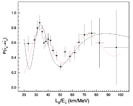
Figure 6: Class 4D (solid lines) and the standard scenario (dashed lines) compared to the KamLAND data. The model parameters are $a_{11}=-9.0\times 10^{-11}$ eV, $a_{12}=0$, $a_{13}=-9\times 10^{-11}$ eV and $r=0.02$.

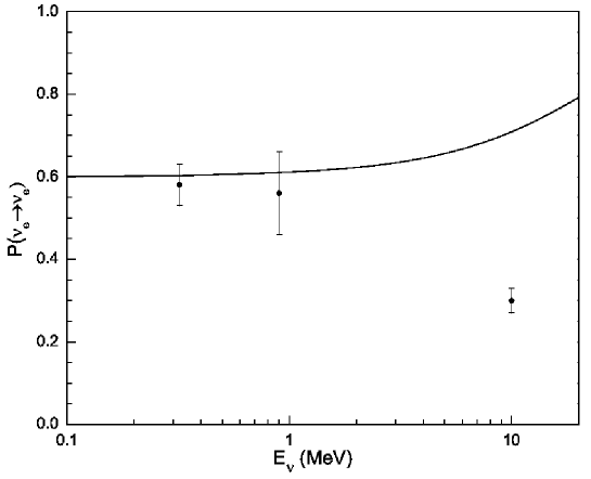
Figure 7: The best fit prediction of Class 4D to the solar data. The model parameters are $a_{11}=9.0\times 10^{-11}$ eV, $a_{12}=0$, $a_{13}=9\times 10^{-11}$ eV and $r=0.02$.

Also, we fit the solar data separately. As was the case for Class 3B, we do not find a good fit to the solar data at high energies (see Fig. 8).

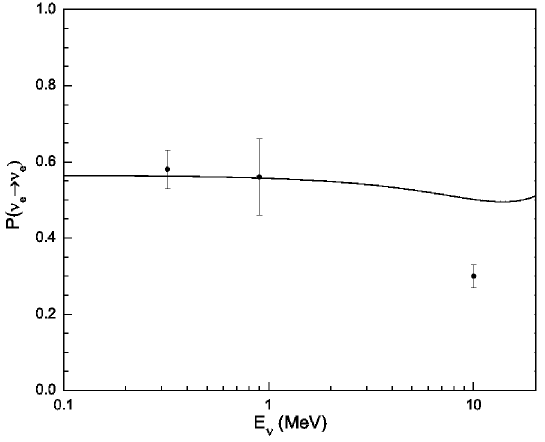
Figure 8: Best fit prediction for survival probability of solar $\nu_{e}$ for Class 4D. The model parameters are $a_{11}=-6.0\times 10^{-11}$ eV, $a_{12}=7.0\times 10^{-11}$ eV, $a_{13}=0.42\times 10^{-11}$ eV and $r=-0.07$.

3.8 Five $c$ parameters

3.8.1 Class 5A

This case has three diagonal and two off-diagonal nonzero $c$. By subtracting a piece proportional to the identity, this case may be reduced to 4B or 4C.

3.8.2 Class 5B

This case has the structure

$$h_{eff}=\pmatrix{c_{11}E+a_{11}&c_{12}E+a_{12}&c_{13}E+a_{13}\cr c_{12}^{*}E+a_{12}^{*}&a_{22}&c_{23}E+a_{23}\cr c_{13}E+a_{13}^{*}&c_{23}E+a_{23}^{*}&c_{33}E+a_{33}}\,,$$ (105)

where $c_{11}$ and $c_{33}$ are real, $c_{13}$ and $c_{23}$ may be taken as real and positive, and $c_{12}$ is complex. At leading order the cubic equation for the eigenvalues of $h_{eff}/E$ is

$$\lambda^{3}-\lambda^{2}(c_{11}+c_{33})+\lambda(c_{11}c_{33}-c_{12}^{2}-c_{13}^{2}-c_{23}^{2})+c_{11}c_{23}^{2}+c_{22}c_{13}^{2}-2c_{12}c_{13}c_{23}c_{\delta}\,,$$ (106)

where the $c_{12}$ is the magnitude and $\delta$ the phase of $c_{12}$. Then we have

$$q = c_{11}^{2}+c_{33}^{2}-c_{11}c_{33}+3(c_{12}^{2}+c_{13}^{2}+c_{23}^{2})\,,$$ (107)

$$r = -2(c_{11}+c_{33})^{3}+9c_{11}c_{33}(c_{11}+c_{33})+9c_{11}(2c_{23}^{2}-c_{12}^{2}-c_{13}^{2})$$ (109)

$$+9c_{33}(2c_{12}^{2}-c_{13}^{2}-c_{23}^{2})-54c_{12}c_{13}c_{23}c_{\delta}\,.$$

and the conditions for a minimum of $f=4q^{3}-r^{2}$ are

$$0 = {\partial f\over\partial c_{11}}=12(2c_{11}-c_{33})q^{2}-2r\left[-6c_{11}^{2}+6c_{11}c_{33}+3c_{33}^{2}+9(2c_{23}^{2}-c_{12}^{2}-c_{13}^{2})\right]\,,$$ (110)

$$0 = {\partial f\over\partial c_{33}}=12(2c_{33}-c_{11})q^{2}-2r\left[-6c_{33}^{2}+6c_{11}c_{33}+3c_{11}^{2}+9(2c_{12}^{2}-c_{13}^{2}-c_{23}^{2})\right]\,,$$ (111)

$$0 = {\partial f\over\partial c_{13}}=72c_{13}q^{2}+36r\left[(c_{11}+c_{33})c_{13}+3c_{12}c_{23}c_{\delta}\right]\,,$$ (112)

$$0 = {\partial f\over\partial c_{12}}=72c_{12}q^{2}+36r\left[(c_{11}-2c_{33})c_{12}+3c_{13}c_{23}c_{\delta}\right]\,,$$ (113)

$$0 = {\partial f\over\partial c_{23}}=72c_{23}q^{2}-36r\left[(2c_{11}-c_{33})c_{23}-3c_{12}c_{13}c_{\delta}\right]\,,$$ (114)

$$0 = {\partial f\over\partial\delta}=-108rc_{12}c_{13}c_{23}\sin\delta\,.$$ (115)

It can be shown by the usual arguments that $q$ and $r$ are not zero, and $c_{\delta}=\pm 1$. By eliminating $q$ and $r$ from Eqs. (112) and (113) we find

$$c_{33}c_{12}c_{13}=c_{\delta}c_{23}(c_{13}^{2}-c_{12}^{2})\,,$$ (116)

and applying a simlar procedure to Eqs. (112) and (114) gives

$$c_{11}c_{13}c_{23}=c_{\delta}c_{12}(c_{13}^{2}-c_{23}^{2})\,.$$ (117)

Using the relations in Eqs. (116) and (117) it can be shown that all minimum conditions are met and that $f=0$, so Eqs. (116) and (117) are the degeneracy conditions. Thus there is a three-parameter set of degeneracies at leading order for this texture. Then, after adding the term $c_{12}c_{23}c_{\delta}/c_{13}$ times the identity, the effective Hamiltonian at leading order may be written as

$$h_{eff}={c_{\delta}\over c_{12}c_{13}c_{23}}\pmatrix{c_{12}^{2}c_{13}^{2}&c_{13}c_{23}c_{12}^{2}&c_{\delta}c_{13}^{2}c_{12}c_{23}\cr c_{13}c_{23}c_{12}^{2}&c_{12}^{2}c_{23}^{2}&c_{\delta}c_{12}c_{13}c_{23}^{2}\cr c_{\delta}c_{13}^{2}c_{12}c_{23}&c_{\delta}c_{12}c_{13}c_{23}^{2}&c_{13}^{2}c_{23}^{2}}E\,.$$ (118)

Without loss of generality $a_{22}$ may be set equal to zero. Then the eigenvalues of $h_{eff}$ to order $E^{0}$ are

$$\lambda_{1}={c_{\delta}S\over c_{12}c_{13}c_{23}}E+a_{11}+a_{33}\,,\qquad\lambda_{2},\lambda_{3}={1\over 2}\left[x\pm\sqrt{x^{2}-4y}\right]\,,$$ (119)

where

$$x \equiv {1\over S}\left[a_{11}c_{23}^{2}(c_{12}^{2}+c_{13}^{2})+a_{33}c_{12}^{2}(c_{13}^{2}+c_{23}^{2})\right.$$ (120)

$$\phantom{{1\over S}}\left.-2{\rm Re}(a_{12})c_{12}^{2}c_{13}c_{23}-2{\rm Re}(a_{13})c_{13}^{2}c_{12}c_{23}c_{\delta}-2{\rm Re}(a_{23})c_{12}c_{13}c_{23}^{2}c_{\delta}\right]\,,$$

$$y \equiv {1\over S^{2}}\left[-2a_{11}{\rm Re}(a_{23})c_{12}c_{13}c_{23}^{2}c_{\delta}-2a_{33}{\rm Re}(a_{12})c_{13}c_{23}c_{12}^{2}+a_{11}a_{33}c_{12}^{2}c_{23}^{2}\right.$$ (121)

$$\phantom{{1\over S}}-c_{13}^{2}c_{23}^{2}|a_{12}|^{2}-c_{12}^{2}c_{13}^{2}|a_{23}|^{2}-c_{12}^{2}c_{23}^{2}|a_{13}|^{2}+2{\rm Re}(a_{13}a_{23})c_{13}c_{23}c_{12}^{2}$$

$$\phantom{{1\over S}}\left.+2{\rm Re}(a_{13}a_{12}^{*})c_{12}c_{13}c_{23}^{2}c_{\delta}+2{\rm Re}(a_{23}a_{12}^{*})c_{12}c_{23}c_{13}^{2}c_{\delta}\right]\,,$$

and $S\equiv c_{12}^{2}c_{13}^{2}+c_{12}^{2}c_{23}^{2}+c_{13}^{2}c_{23}^{2}$. Thus degeneracy requires that the quadratic discriminant $g=x^{2}-4y$ be zero. It can be shown that $g$ has a minimum at zero when

$$y_{12} = c_{\delta}c_{12}\left(\frac{y_{13}}{c_{13}}-\frac{y_{23}}{c_{23}}\right)\,,$$ (122)

$$x_{12} = \frac{c_{23}a_{11}}{2c_{13}}+c_{\delta}\frac{c_{12}(c_{13}^{2}+c_{23}^{2})}{c_{23}(c_{12}^{2}+c_{13}^{2})}\left(x_{23}-\frac{c_{\delta}c_{12}c_{33}}{2c_{13}}\right)\,,$$ (123)

$$x_{13} = c_{\delta}\frac{c_{12}^{2}a_{33}+c_{23}^{2}a_{11}}{2c_{12}c_{23}}+\frac{c_{13}(c_{12}^{2}+c_{23}^{2})}{c_{23}(c_{12}^{2}+c_{13}^{2})}\left(x_{23}-\frac{c_{\delta}c_{12}c_{33}}{2c_{13}}\right)\,,$$ (124)

where $x_{ij}={\rm Re}(a_{ij})$, and $y_{ij}={\rm Im}(a_{ij})$; these are the degeneracy conditions. The eigenvalues to order $E^{-1}$ are then

$$\lambda_{1} = {c_{\delta}SE\over c_{12}c_{13}c_{23}}+-{1\over SE}c_{\delta}c_{12}c_{13}c_{23}\left[a_{11}a_{33}-|a_{12}|^{2}-|a_{13}|^{2}-|a_{23}|^{2}\right]\,,$$ (125)

$$\lambda_{2} = {1\over SE}c_{\delta}c_{12}c_{13}c_{23}\left[a_{11}a_{33}-|a_{12}|^{2}-|a_{13}|^{2}-|a_{23}|^{2}\right]\,,\qquad\lambda_{3}=0\,,$$ (126)

and to leading order the mixing matrix that diagonalizes $h_{eff}$ is

$$U=\pmatrix{\cos\theta\cos\phi&-\cos\xi\sin\phi-\sin\xi\sin\theta\cos\phi&\sin\xi\sin\phi-\cos\xi\sin\theta\cos\phi\cr\sin\theta&\cos\theta\sin\xi&\cos\theta\cos\xi\cr\cos\theta\sin\phi&\cos\xi\cos\phi-\sin\xi\sin\theta\sin\phi&-\sin\xi\cos\phi-\cos\xi\sin\theta\sin\phi}\,,$$ (127)

where

$$\sin\theta \equiv {1\over\sqrt{S}}c_{12}c_{23}\,,\qquad\sin\phi\equiv{c_{23}\over\sqrt{c_{12}^{2}+c_{23}^{2}}}\,,$$ (128)

$$\sin\xi \equiv c_{\delta}{c_{12}^{2}c_{23}^{2}(a_{11}+a_{33})\over N_{3}\sqrt{c_{12}^{2}+c_{23}^{2}}}\,,\qquad\cos\xi={\sqrt{S}\over N_{3}}{c_{23}^{2}a_{11}-c_{12}^{2}a_{33}\over\sqrt{c_{23}^{2}+c_{12}^{2}}}\,,$$ (129)

and

$$N_{3}^{2}=a_{33}^{2}c_{12}^{4}(c_{13}^{2}+c_{23}^{2})+a_{11}^{2}c_{23}^{4}(c_{12}^{2}+c_{13}^{2})-2a_{11}a_{33}c_{13}^{2}c_{12}^{2}c_{23}^{2}\,,$$ (130)

is a normalization factor. The oscillation probabilities are

$$P(\nu_{\mu}\to\nu_{\mu}) = 1-\sin^{2}\xi\sin^{2}2\theta\sin^{2}\left(\Delta_{21}{L\over 2}\right)-\cos^{2}\xi\sin^{2}2\theta\sin^{2}\left(\Delta_{31}{L\over 2}\right)$$ (131)

$$\phantom{1}-\cos^{4}\theta\sin^{2}2\xi\sin^{2}\left(\Delta_{32}{L\over 2}\right)\,,$$

$$P(\nu_{\mu}\to\nu_{e}) = 2\sin 2\theta\cos\theta\cos\phi\sin\xi(\cos\xi\sin\phi+\sin\xi\sin\theta\cos\phi)\sin^{2}\left(\Delta_{21}{L\over 2}\right)$$ (132)

$$-2\sin 2\theta\cos\theta\cos\phi\cos\xi(\sin\xi\sin\phi-\cos\xi\sin\theta\cos\phi)\sin^{2}\left(\Delta_{31}{L\over 2}\right)$$

$$+2\sin 2\xi\cos^{2}\theta(\cos\xi\sin\phi+\sin\xi\sin\theta\cos\phi)(\sin\xi\sin\phi-\cos\xi\sin\theta\cos\phi)$$

$$\times\sin^{2}\left(\Delta_{32}{L\over 2}\right)\,.$$

In order to have nearly maximal $\nu_{\mu}$ oscillations at the atmospheric scale, the $\Delta_{32}$ term must have amplitude close to unity, or $\theta\simeq 0,\pi$ and $\xi\simeq\pi/4$. Then from Eq. (129)

$$a_{33}c_{12}(c_{12}+c_{\delta}c_{23}\sin\theta)\simeq a_{11}c_{23}(c_{23}-c_{\delta}c_{12}\sin\theta)\,.$$ (133)

The small value of $\sin\theta$ implies $c_{12}^{2},c_{23}^{2}\ll c_{13}^{2}$. Furthermore, in order to have small $\nu_{\mu}\to\nu_{e}$ oscillations at the $\Delta_{32}$ scale, $\sin^{2}\phi\ll 1$, or $c_{23}^{2}\ll c_{12}^{2}$, i.e., there is a hierarchy among the off-diagonal $c_{ij}$. Then Eq. (133) implies $a_{33}\ll a_{11}$ as well. Therefore there is a lot of fine tuning required to achieve the proper mixing.

For simplicity, we only considered the parameters as real numbers. We have scanned the $c_{12}$, $c_{13}$ and $c_{23}$ parameter space to fit the KamLAND and solar data. Other parameters in the Hamiltonian can be determined by these three parameters, i.e., $c_{11}$ and $c_{13}$ can be determined from Eqs. (116) and (117). Also, for the atmospheric and long-baseline neutrinos, the $\Delta_{23}$ term has the correct energy dependence, and gives

$$\delta m_{eff}^{2}=2E\Delta_{23}=\frac{2}{S}c_{\delta}c_{12}c_{13}c_{23}[a_{11}a_{33}-|a_{12}|^{2}-|a_{13}|^{2}-|a_{23}|^{2}]\,.$$ (134)

The above equation together with Eqs. (124) and (133) determine all $a_{ij}$. Another constraint is the hierarchy among the off-diagonal $c_{ij}$, $c_{23}^{2}\ll c_{12}^{2}\ll c_{13}^{2}$, which is also considered during the parameter search.

We have varied the range of $c_{13}$ from the order of $10^{-20}$ to $10^{-16}$ and take $c_{12}$ and $c_{23}$ to be at least one order of magnitude less than $c_{13}$ and $c_{12}$ respectively. We found parameter values that can fit the KamLAND data (see Fig. 9), but they do not yield reasonable agreement with the solar data at high energies (see Fig. 10). We also attempted to fit solar neutrinos alone and found there are no parameter values that can yield reasonable agreement with the solar data. The best fit is shown in Fig. 11.

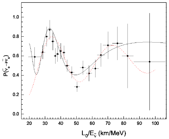
Figure 9: Best fits for Class 5B (solid lines) and for standard oscillations (dashed lines) compared to the KamLAND data. The model parameters are $c_{23}=5.9\times 10^{-23}$, $c_{12}=1.0\times 10^{-22}$ and $c_{13}=8.9\times 10^{-19}$.

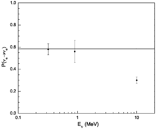
Figure 10: The prediction of Class 5B for the solar neutrino survival probability using the parameter values obtained from fitting the KamLAND data.

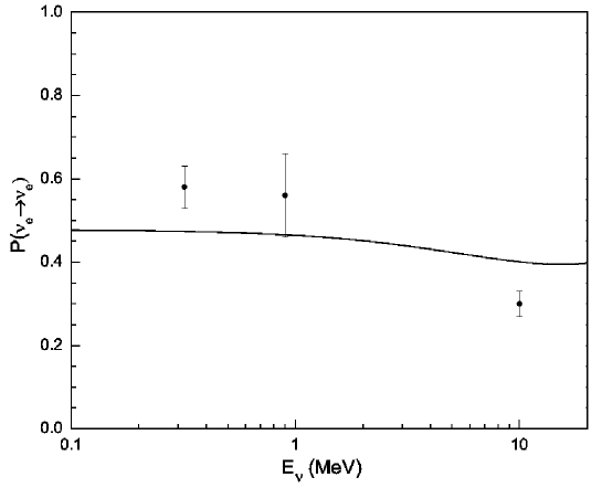
Figure 11: Best fit prediction for the $\nu_{e}$ survival probability in Class 5B. The model parameters for the best fit are $c_{23}=1.0\times 10^{-18}$, $c_{12}=2.4\times 10^{-18}$ and $c_{13}=1.0\times 10^{-18}$.

3.9 Six $c$ parameters

In this case all $c$ elements are nonzero. By subtracting off a piece proportional to the identity, this case may be reduced to Class 5B, which is ruled out.

4 Summary

We have examined the general three neutrino effective Hamiltonian in Eq. (1) for the case of direction-independent interactions and no neutrino mass. We looked for texture classes in which two eigenvalues were degenerate to order $1/E$ at high neutrino energy, so that oscillations of atmospheric and long-baseline neutrinos would exhibit the usual $L/E$ dependence.

Among the classes that had the proper $1/E$ dependence at high energy, none was also able to fit the atmospheric, long-baseline, solar and KamLAND data simultaneously. Class 1A (along with the equivalent Classes 2A and 3A) reduced to the direction-independent bicycle model, which has been shown to be inconsistent with the solar, atmospheric and long-baseline neutrino data. Classes 2C (and the equivalent 3E) and 3F did not have the proper oscillation amplitudes for atmospheric neutrinos. Finally, Classes 3B (and the equivalent Classes 3C, 4A and 4D) and 5B (and the equivalent Class 6) were able to fit atmospheric and long-baseline neutrino data, but could not simultaneously fit KamLAND and solar data at lower neutrino energies. The major difficulty in these latter classes was reproducing the low survival probability of high-energy solar neutrinos.

Although we have not made an exhaustive search of the parameter space, the fact that high-energy neutrinos exhibit an $L/E$ dependence in their oscillations over many orders of magnitude in $E$ suggests that the only way this can occur in the effective Hamiltonian described by Eq. (1) is via the degeneracy of two eigenvalues to order $1/E$. Since none of the cases where such a degeneracy occurs are also able to fit all neutrino data simultaneously, it seems extremely unlikely that any direction-independent SME model without neutrino mass will provide a viable description of all neutrino oscillation phenmomena. There is also strong evidence against direction-dependent terms. Furthermore, nonrenormalizable Lorentz noninvariant effective Hamiltonians with higher powers of energy (as in, e.g., the model of Ref. [9]) and no neutrino masses would require additional degeneracy conditions. Therefore it appears highly unlikely that Lorentz invariance violation alone can account for all of the observed oscillation phenomena.

References

- [1] See, e.g., V. Barger, D. Marfatia and K. Whisnant, Int. J. Mod. Phys. E 12, 569 (2003) [arXiv:hep-ph/0308123]; S. Pakvasa and J. W. F. Valle, Proc. Indian Natl. Sci. Acad. 70A, 189 (2004) [arXiv:hep-ph/0301061].
- [2] D. Colladay, V. A. Kostelecky, Phys. Rev. D55, 6760-6774 (1997) [hep-ph/9703464]; Phys. Rev. D58, 116002 (1998) [hep-ph/9809521].
- [3] S. R. Coleman and S. L. Glashow, Phys. Rev. D 59, 116008 (1999) [arXiv:hep-ph/9812418].
- [4] V. D. Barger, S. Pakvasa, T. J. Weiler and K. Whisnant, Phys. Rev. Lett. 85, 5055 (2000) [arXiv:hep-ph/0005197].
- [5] T. Katori, V. A. Kostelecky and R. Tayloe, Phys. Rev. D 74, 105009 (2006) [arXiv:hep-ph/0606154].
- [6] V. A. Kostelecky and M. Mewes, Phys. Rev. D 70, 031902 (2004) [arXiv:hep-ph/0308300].
- [7] V. A. Kostelecky and M. Mewes, Phys. Rev. D 69, 016005 (2004) [arXiv:hep-ph/0309025].
- [8] V. Barger, D. Marfatia and K. Whisnant, Phys. Lett. B 653, 267 (2007) [arXiv:0706.1085 [hep-ph]].
- [9] J. S. Diaz and A. Kostelecky, Phys. Lett. B 700, 25 (2011) [arXiv:1012.5985 [hep-ph]].
- [10] C. Athanassopoulos et al. [LSND Collaboration], Phys. Rev. C 54, 2685 (1996) [arXiv:nucl-ex/9605001]; Phys. Rev. Lett. 77, 3082 (1996) [arXiv:nucl-ex/9605003]; Phys. Rev. C 58, 2489 (1998) [arXiv:nucl-ex/9706006]; Phys. Rev. Lett. 81, 1774 (1998) [arXiv:nucl-ex/9709006]; A. Aguilar et al. [LSND Collaboration], Phys. Rev. D 64, 112007 (2001) [arXiv:hep-ex/0104049].
- [11] A. A. Aguilar-Arevalo et al. [MiniBooNE Collaboration], Phys. Rev. Lett. 102, 101802 (2009) [arXiv:0812.2243 [hep-ex]]; Phys. Rev. Lett. 103, 111801 (2009) [arXiv:0904.1958 [hep-ex]]; arXiv:1007.1150 [hep-ex].
- [12] L. B. Auerbach et al. [LSND Collaboration], Phys. Rev. D 72, 076004 (2005) [arXiv:hep-ex/0506067]; P. Adamson et al. [MINOS Collaboration], Phys. Rev. Lett. 101, 151601 (2008) [arXiv:0806.4945 [hep-ex]]; Phys. Rev. Lett. 105, 151601 (2010) [arXiv:1007.2791 [hep-ex]]; T. Katori [MiniBooNE Collaboration], arXiv:1008.0906 [hep-ph].
- [13] L. Wolfenstein, Phys. Rev. D 17, 2369 (1978); V. D. Barger, K. Whisnant, S. Pakvasa and R. J. Phillips, Phys. Rev. D 22, 2718 (1980); P. Langacker, J. P. Leveille and J. Sheiman, Phys. Rev. D 27, 1228 (1983).
- [14] S. N. Ahmed et al. [SNO Collaboration], Phys. Rev. Lett. 92, 181301 (2004) [arXiv:nucl-ex/0309004]; B. Aharmim et al. [SNO Collaboration], Phys. Rev. C 72, 055502 (2005) [arXiv:nucl-ex/0502021]; Phys. Rev. C 75, 045502 (2007) [arXiv:nucl-ex/0610020]; Phys. Rev. Lett. 101, 111301 (2008) [arXiv:0806.0989 [nucl-ex]]; Phys. Rev. C 81, 055504 (2010) [arXiv:0910.2984 [nucl-ex]].
- [15] See, e.g., the global fits to neutrino data in T. Schwetz, M. A. Tortola and J. W. F. Valle, New J. Phys. 10, 113011 (2008) [arXiv:0808.2016 [hep-ph]] (version 3 of the preprint, dated Feb. 11, 2010, presented an updated global analysis); M. C. Gonzalez-Garcia, M. Maltoni, J. Salvado, JHEP 1004, 056 (2010). [arXiv:1001.4524 [hep-ph]].
- [16] Y. Ashie et al. [Super-Kamiokande Collaboration], Phys. Rev. Lett. 93, 101801 (2004) [arXiv:hep-ex/0404034].
- [17] S. Yamamoto et al. [K2K Collaboration], Phys. Rev. Lett. 96, 181801 (2006) [arXiv:hep-ex/0603004].
- [18] P. Adamson et al. [The MINOS Collaboration], Phys. Rev. D82, 051102 (2010) [arXiv:1006.0996 [hep-ex]]; Phys. Rev. Lett. 103, 261802 (2009). [arXiv:0909.4996 [hep-ex]].
- [19] K. Abe et al. [T2K Collaboration], arXiv:1106.2822 [hep-ex].
- [20] T. Araki et al. [KamLAND Collaboration], Phys. Rev. Lett. 94, 081801 (2005) [arXiv:hep-ex/0406035].
- [21] V. Barger, D. Marfatia and K. Whisnant, Phys. Lett. B 617, 78 (2005) [arXiv:hep-ph/0501247].
- [22] S. Avvakumov et al., Phys. Rev. Lett. 89, 011804 (2002) [arXiv:hep-ex/0203018].