Distributional Results for Thresholding Estimators in High-Dimensional Gaussian Regression Models

Abstract

We study the distribution of hard-, soft-, and adaptive soft-thresholding estimators within a linear regression model where the number of parameters $k$ can depend on sample size $n$ and may diverge with $n$. In addition to the case of known error-variance, we define and study versions of the estimators when the error-variance is unknown. We derive the finite-sample distribution of each estimator and study its behavior in the large-sample limit, also investigating the effects of having to estimate the variance when the degrees of freedom $n-k$ does not tend to infinity or tends to infinity very slowly. Our analysis encompasses both the case where the estimators are tuned to perform consistent variable selection and the case where the estimators are tuned to perform conservative variable selection. Furthermore, we discuss consistency, uniform consistency and derive the uniform convergence rate under either type of tuning.

MSC subject classification: 62F11, 62F12, 62J05, 62J07, 62E15, 62E20

Keywords and phrases: Thresholding, Lasso, adaptive Lasso, penalized maximum likelihood, variable selection, finite-sample distribution, asymptotic distribution, variance estimation, uniform convergence rate, high-dimensional model, oracle property

1 Introduction

We study the distribution of thresholding estimators such as hard-thresholding, soft-thresholding, and adaptive soft-thresholding in a linear regression model when the number of regressors can be large. These estimators can be viewed as penalized least-squares estimators in the case of an orthogonal design matrix, with soft-thresholding then coinciding with the Lasso (introduced by Frank and Friedman (1993), Alliney and Ruzinsky (1994), and Tibshirani (1996)) and with adaptive soft-thresholding coinciding with the adaptive Lasso (introduced by Zou (2006)). Thresholding estimators have of course been discussed earlier in the context of model selection (see Bauer, Pötscher and Hackl (1988)) and in the context of wavelets (see, e.g., Donoho, Johnstone, Kerkyacharian, Picard (1995)). Contributions concerning distributional properties of thresholding and penalized least-squares estimators are as follows: Knight and Fu (2000) study the asymptotic distribution of the Lasso estimator when it is tuned to act as a conservative variable selection procedure, whereas Zou (2006) studies the asymptotic distribution of the Lasso and the adaptive Lasso estimators when they are tuned to act as consistent variable selection procedures. Fan and Li (2001) and Fan and Peng (2004) study the asymptotic distribution of the so-called smoothly clipped absolute deviation (SCAD) estimator when it is tuned to act as a consistent variable selection procedure. In the wake of Fan and Li (2001) and Fan and Peng (2004) a large number of papers have been published that derive the asymptotic distribution of various penalized maximum likelihood estimators under consistent tuning; see the introduction in Pötscher and Schneider (2009) for a partial list. Except for Knight and Fu (2000), all these papers derive the asymptotic distribution in a fixed-parameter framework. As pointed out in Leeb and Pötscher (2005), such a fixed-parameter framework is often highly misleading in the context of variable selection procedures and penalized maximum likelihood estimators. For that reason, Pötscher and Leeb (2009) and Pötscher and Schneider (2009) have conducted a detailed study of the finite-sample as well as large-sample distribution of various penalized least-squares estimators, adopting a moving-parameter framework for the asymptotic results. [Related results for so-called post-model-selection estimators can be found in Leeb and Pötscher (2003, 2005) and for model averaging estimators in Pötscher (2006); see also Sen (1979) and Pötscher (1991).] The papers by Pötscher and Leeb (2009) and Pötscher and Schneider (2009) are set in the framework of an orthogonal linear regression model with a fixed number of parameters and with the error-variance being known.

In the present paper we build on the just mentioned papers Pötscher and Leeb (2009) and Pötscher and Schneider (2009). In contrast to these papers, we do not assume the number of regressors $k$ to be fixed, but let it depend on sample size – thus allowing for high-dimensional models. We also consider the case where the error-variance is unknown, which in case of a high-dimensional model creates non-trivial complications as then estimators for the error-variance will typically not be consistent. Considering thresholding estimators from the outset in the present paper allows us also to cover non-orthogonal design. While the asymptotic distributional results in the known-variance case do not differ in substance from the results in Pötscher and Leeb (2009) and Pötscher and Schneider (2009), not unexpectedly we observe different asymptotic behavior in the unknown-variance case if the number of degrees of freedom $n-k$ is constant, the difference resulting from the non-vanishing variability of the error-variance estimator in the limit. Less expected is the result that – under consistent tuning – for the variable selection probabilities (implied by all the estimators considered) as well as for the distribution of the hard-thresholding estimator, estimation of the error-variance still has an effect asymptotically even if $n-k$ diverges, but does so only slowly.

To give some idea of the theoretical results obtained in the paper we next present a rough summary of some of these results. For simplicity of exposition assume for the moment that the $n\times k$ design matrix $X$ is such that the diagonal elements of $(X^{\prime}X/n)^{-1}$ are equal to $1$, and that the error-variance $\sigma^{2}$ is equal to $1$. Let $\tilde{\theta}_{H,i}$ denote the hard-thresholding estimator for the $i$-th component $\theta_{i}$ of the regression parameter, the threshold being given by $\hat{\sigma}\eta_{i,n}$, with $\hat{\sigma}^{2}$ denoting the usual error-variance estimator and with $\eta_{i,n}$ denoting a tuning parameter. An infeasible version of the estimator, denoted by $\hat{\theta}_{H,i}$, which uses $\sigma$ instead of $\hat{\sigma}$, is also considered (known-variance case). We then show that the uniform rate of convergence of the hard-thresholding estimator is $n^{-1/2}$ if the threshold satisfies $\eta_{i,n}\rightarrow 0$ and $n^{1/2}\eta_{i,n}\rightarrow e_{i}<\infty$ (”conservative tuning”), but that the uniform rate is only $\eta_{i,n}$ if the threshold satisfies $\eta_{i,n}\rightarrow 0$ and $n^{1/2}\eta_{i,n}\rightarrow\infty$ (”consistent tuning”). The same result also holds for the soft-thresholding estimator $\tilde{\theta}_{S,i}$ and the adaptive soft-thresholding estimator $\tilde{\theta}_{AS,i}$, as well as for infeasible variants of the estimators that use knowledge of $\sigma$ (known-variance case). Furthermore, all possible limits of the centered and scaled distribution of the hard-thresholding estimator $\tilde{\theta}_{H,i}$ (as well as of the soft- and the adaptive soft-thresholding estimators $\tilde{\theta}_{S,i}$ and $\tilde{\theta}_{AS,i}$) under a moving parameter framework are obtained. Consider first the case of conservative tuning: then all possible limiting forms of the distribution of $n^{1/2}\left(\tilde{\theta}_{H,i}-\theta_{i,n}\right)$ as well as of $n^{1/2}\left(\hat{\theta}_{H,i}-\theta_{i,n}\right)$ for arbitrary parameter sequences $\theta_{i,n}$ are determined. It turns out that – in the known-variance case – these limits are of the same functional form as the finite-sample distribution, i.e., they are a convex combination of a pointmass and an absolutely continuous distribution that is an excised version of a normal distribution. In the unknown-variance case, when the number of degrees of freedom $n-k$ goes to infinity, exactly the same limits arise. However, if $n-k$ is constant, the limits are ”averaged” versions of the limits in the known-variance case, the averaging being with respect to the distribution of the variance estimator $\hat{\sigma}^{2}$. Again these limits have the same functional form as the corresponding finite-sample distributions. Consider next the case of consistent tuning: Here the possible limits of $\eta_{i,n}^{-1}\left(\tilde{\theta}_{H,i}-\theta_{i,n}\right)$ as well as of $\eta_{i,n}^{-1}\left(\hat{\theta}_{H,i}-\theta_{i,n}\right)$ have to be considered, as $\eta_{i,n}$ is the uniform convergence rate. In the known-variance case the limits are convex combinations of (at most) two pointmasses, the location of the pointmasses as well as the weights depending on $\theta_{i,n}$ and $\eta_{i,n}$. In the unknown-variance case exactly the same limits arise if $n-k$ diverges to infinity sufficiently fast; however, if $n-k$ is constant or diverges to infinity sufficiently slowly, the limits are again convex combinations of the same pointmasses, but with weights that are typically different. The picture for soft-thresholding and adaptive soft-thresholding is somewhat different: in the known-variance case, as well as in the unknown-variance case when $n-k$ diverges to infinity, the limits are (single) pointmasses. However, in the unknown-variance case and if $n-k$ is constant, the limit distribution can have an absolutely continuous component. It is furthermore useful to point out that in case of consistent tuning the sequence of distributions of $n^{1/2}\left(\tilde{\theta}_{H,i}-\theta_{i,n}\right)$ is not stochastically bounded in general (since $\eta_{i,n}$ is the uniform convergence rate), and the same is true for soft-thresholding $\tilde{\theta}_{S,i}$ and adaptive soft-thresholding $\tilde{\theta}_{AS,i}$. This throws a light on the fragility of the oracle-property, see Section 6.4 for more discussion.

While our theoretical results for the thresholding estimators immediately apply to Lasso and adaptive Lasso in case of orthogonal design, this is not so in the non-orthogonal case. In order to get some insight into the finite-sample distribution of the latter estimators also in the non-orthogonal case, we numerically compare the distribution of Lasso and adaptive Lasso with their thresholding counterparts in a simulation study.

The main take-away messages of the paper can be summarized as follows:

• The finite-sample distributions of the various thresholding estimators considered are highly non-normal, the distributions being in each case a convex combination of pointmass and an absolutely continuous (non-normal) component.

• The non-normality persists asymptotically in a moving parameter framework.

• Results in the unknown-variance case are obtained from the corresponding results in the known-variance case by smoothing with respect to the distribution of $\hat{\sigma}$. In line with this, one would expect the limiting behavior in the unknown-variance case to coincide with the limiting behavior in the known-variance whenever the degrees of freedom $n-k$ diverge to infinity. This indeed turns out to be so for some of the results, but not for others where we see that the speed of divergence of $n-k$ matters.

• In case of conservative tuning the estimators have the expected uniform convergence rate, which is $n^{-1/2}$ under the simplified assumptions of the above discussion, whereas under consistent tuning the uniform rate is slower, namely $\eta_{i,n}$ under the simplified assumptions of the above discussion. This is intimately connected with the fact that the so-called ‘oracle property’ paints a misleading picture of the performance of the estimators.

• The numerical study suggests that the results for the thresholding estimators $\tilde{\theta}_{S,i}$ and $\tilde{\theta}_{AS,i}$ qualitatively apply also to the (components of) the Lasso and the adaptive Lasso as long as the design matrix is not too ill-conditioned.

The paper is organized as follows. We introduce the model and define the estimators in Section 2. Section 3 treats the variable selection probabilities implied by the estimators. Consistency, uniform consistency, and uniform convergence rates are discussed in Section 4. We derive the finite-sample distribution of each estimator in Section 5 and study the large-sample behavior of these in Section 6. A numerical study of the finite-sample distribution of Lasso and adaptive Lasso can be found in Section 7. All proofs are relegated to Section 8.

2 The Model and the Estimators

Consider the linear regression model

$$Y=X\theta+u$$

with $Y$ an $n\times 1$ vector, $X$ a nonstochastic $n\times k$ matrix of rank $k\geq 1$, and $u\sim N(0,\sigma^{2}I_{n})$, $0<\sigma<\infty$. We allow $k$, the number of columns of $X$, as well as the entries of $Y$, $X$, and $u$ to depend on sample size $n$ (in fact, also the probability spaces supporting $Y$ and $u$ may depend on $n$), although we shall almost always suppress this dependence on $n$ in the notation. Note that this framework allows for high-dimensional regression models, where the number of regressors $k$ is large compared to sample size $n$, as well as for the more classical situation where $k$ is much smaller than $n$. Furthermore, let $\xi_{i,n}$ denote the nonnegative square root of $((X^{\prime}X/n)^{-1})_{ii}$, the $i$-th diagonal element of $(X^{\prime}X/n)^{-1}$. Now let

$$\hat{\theta}_{LS}=\left(X^{\prime}X\right)^{-1}X^{\prime}Y$$

$$\hat{\sigma}^{2}=(n-k)^{-1}(Y-X\hat{\theta}_{LS})^{\prime}(Y-X\hat{\theta}_{LS})$$

denote the least-squares estimator for $\theta$ and the associated estimator for $\sigma^{2}$, the latter being defined only if $n>k$. The hard-thresholding estimator $\tilde{\theta}_{H}$ is defined via its components as follows

$$\tilde{\theta}_{H,i}=\tilde{\theta}_{H,i}(\eta_{i,n})=\hat{\theta}_{LS,i}\boldsymbol{1}\left(\left|\hat{\theta}_{LS,i}\right|>\hat{\sigma}\xi_{i,n}\eta_{i,n}\right),$$

where the tuning parameters $\eta_{i,n}$ are positive real numbers and $\hat{\theta}_{LS,i}$ denotes the $i$-th component of the least-squares estimator. We shall also need to consider its infeasible counterpart $\hat{\theta}_{H}$ given by

$$\hat{\theta}_{H,i}=\hat{\theta}_{H,i}(\eta_{i,n})=\hat{\theta}_{LS,i}\boldsymbol{1}\left(\left|\hat{\theta}_{LS,i}\right|>\sigma\xi_{i,n}\eta_{i,n}\right).$$

The soft-thresholding estimator $\tilde{\theta}_{S}$ and its infeasible counterpart $\hat{\theta}_{S}$ are given by

$$\tilde{\theta}_{S,i}=\tilde{\theta}_{S,i}(\eta_{i,n})=\mathop{\mathrm{s}ign}(\hat{\theta}_{LS,i})\left(\left|\hat{\theta}_{LS,i}\right|-\hat{\sigma}\xi_{i,n}\eta_{i,n}\right)_{+}$$

and

$$\hat{\theta}_{S,i}=\hat{\theta}_{S,i}(\eta_{i,n})=\mathop{\mathrm{s}ign}(\hat{\theta}_{LS,i})\left(\left|\hat{\theta}_{LS,i}\right|-\sigma\xi_{i,n}\eta_{i,n}\right)_{+},$$

where $\left(\cdot\right)_{+}=\max(\cdot,0)$. Finally, the adaptive soft-thresholding estimator $\tilde{\theta}_{AS}$ and its infeasible counterpart $\hat{\theta}_{AS}$ are defined via

$$\tilde{\theta}_{AS,i} = \tilde{\theta}_{AS,i}(\eta_{i,n})=\hat{\theta}_{LS,i}\left(1-\hat{\sigma}^{2}\xi_{i,n}^{2}\eta_{i,n}^{2}/\hat{\theta}_{LS,i}^{2}\right)_{+}$$

$$= \left\{\begin{array}[]{cc}0&\text{if }\left|\hat{\theta}_{LS,i}\right|\leq\hat{\sigma}\xi_{i,n}\eta_{i,n}\\ \hat{\theta}_{LS,i}-\hat{\sigma}^{2}\xi_{i,n}^{2}\eta_{i,n}^{2}/\hat{\theta}_{LS,i}&\text{if }\left|\hat{\theta}_{LS,i}\right|>\hat{\sigma}\xi_{i,n}\eta_{i,n}\end{array}\right.$$

and

$$\hat{\theta}_{AS,i} = \hat{\theta}_{AS,i}(\eta_{i,n})=\hat{\theta}_{LS,i}\left(1-\sigma^{2}\xi_{i,n}^{2}\eta_{i,n}^{2}/\hat{\theta}_{LS,i}^{2}\right)_{+}$$

$$= \left\{\begin{array}[]{cc}0&\text{if }\left|\hat{\theta}_{LS,i}\right|\leq\sigma\xi_{i,n}\eta_{i,n}\\ \hat{\theta}_{LS,i}-\sigma^{2}\xi_{i,n}^{2}\eta_{i,n}^{2}/\hat{\theta}_{LS,i}&\text{if }\left|\hat{\theta}_{LS,i}\right|>\sigma\xi_{i,n}\eta_{i,n}\end{array}\right..$$

Note that $\tilde{\theta}_{H}$, $\tilde{\theta}_{S}$, and $\tilde{\theta}_{AS}$ as well as their infeasible counterparts are equivariant under scaling of the columns of $(Y:X)$ by non-zero column-specific scale factors. We have chosen to let the thresholds $\hat{\sigma}\xi_{i,n}\eta_{i,n}$ ($\sigma\xi_{i,n}\eta_{i,n}$, respectively) depend explicitly on $\hat{\sigma}$ ($\sigma$, respectively) and $\xi_{i,n}$ in order to give $\eta_{i,n}$ an interpretation independent of the values of $\sigma$ and $X$. Furthermore, often $\eta_{i,n}$ will be chosen independently of $i$, i.e., $\eta_{i,n}=\eta_{n}$ where $\eta_{n}$ is a positive real number. Clearly, for the feasible versions we always need to assume $n>k$, whereas for the infeasible versions $n\geq k$ suffices.

We note the simple fact that

$$0\leq\tilde{\theta}_{S,i}\leq\tilde{\theta}_{AS,i}\leq\tilde{\theta}_{H,i}\leq\hat{\theta}_{LS,i}$$ (3)

holds on the event that $\hat{\theta}_{LS,i}\geq 0$, and that

$$\hat{\theta}_{LS,i}\leq\tilde{\theta}_{H,i}\leq\tilde{\theta}_{AS,i}\leq\tilde{\theta}_{S,i}\leq 0$$ (4)

holds on the event that $\hat{\theta}_{LS,i}\leq 0$. Analogous inequalities hold for the infeasible versions of the estimators.

Remark 1

(Lasso) (i) Consider the objective function

$$(Y-X\theta)^{\prime}(Y-X\theta)+2n\hat{\sigma}\sum_{i=1}^{k}\eta_{i,n}^{\prime}\left|\theta_{i}\right|,$$

where $\eta_{i,n}^{\prime}$ are positive real numbers. It is well-known that a unique minimizer $\tilde{\theta}_{L}$ of this objective function exists, the Lasso-estimator. It is easy to see that in case $X^{\prime}X$ is diagonal we have

$$\tilde{\theta}_{L,i}=\mathop{\mathrm{s}ign}(\hat{\theta}_{LS,i})\left(\left|\hat{\theta}_{LS,i}\right|-\hat{\sigma}\eta_{i,n}^{\prime}\xi_{i,n}^{2}\right)_{+}.$$

Hence, in the case of diagonal $X^{\prime}X$, the components $\tilde{\theta}_{L,i}$ of the Lasso reduce to soft-thresholding estimators with appropriate thresholds; in particular, $\tilde{\theta}_{L,i}$ coincides with $\tilde{\theta}_{S,i}$ for the choice $\eta_{i,n}^{\prime}=\eta_{i,n}\xi_{i,n}^{-1}$. Therefore all results derived below for soft-thresholding immediately give corresponding results for the Lasso as well as for the Dantzig-selector in the diagonal case. We shall abstain from spelling out further details.

(ii) Sometimes $\eta_{i,n}^{\prime}$ in the definition of the Lasso is chosen independently of $i$; more reasonable choices seem to be (a) $\eta_{i,n}^{\prime}=\eta_{i,n}\psi_{i,n}$ (where $\psi_{i,n}$ denotes the nonnegative square root of the $i$-th diagonal element of $(X^{\prime}X/n)$), and (b) $\eta_{i,n}^{\prime}=\eta_{i,n}\xi_{i,n}^{-1}$ where $\eta_{i,n}$ are positive real numbers (not depending on the design matrix and often not on $i$) as then $\eta_{i,n}$ again has an interpretation independent of the values of $\sigma$ and $X$. Note that in case (a) or (b) the solution of the optimization problem is equivariant under scaling of the columns of $(Y:X)$ by non-zero column-specific scale factors.

(iii) Similar results obviously hold for the infeasible versions of the estimators.

Remark 2

(Adaptive Lasso) Consider the objective function

$$(Y-X\theta)^{\prime}(Y-X\theta)+2n\hat{\sigma}^{2}\sum_{i=1}^{k}(\eta_{i,n}^{\prime})^{2}\left|\theta_{i}\right|/\left|\hat{\theta}_{LS,i}\right|,$$

where $\eta_{i,n}^{\prime}$ are positive real numbers. This is the objective function of the adaptive Lasso (where often $\eta_{i,n}^{\prime}=\eta_{n}^{\prime}$ is chosen independent of $i$). Again the minimizer $\tilde{\theta}_{AL}$ exists and is unique (at least on the event where $\hat{\theta}_{LS,i}\neq 0$ for all $i$). Clearly, $\tilde{\theta}_{AL}$ is equivariant under scaling of the columns of $(Y:X)$ by non-zero column-specific scale factors provided $\eta_{i,n}^{\prime}$ does not depend on the design matrix. It is easy to see that in case $X^{\prime}X$ is diagonal we have

$$\tilde{\theta}_{AL,i}=\hat{\theta}_{LS,i}\left(1-\hat{\sigma}^{2}\xi_{i,n}^{2}\left(\eta_{i,n}^{\prime}\right)^{2}/\hat{\theta}_{LS,i}^{2}\right)_{+}.$$

Hence, in the case of diagonal $X^{\prime}X$, the components $\tilde{\theta}_{AL,i}$ of the adaptive Lasso reduce to the adaptive soft-thresholding estimators $\tilde{\theta}_{AS,i}$ (for $\eta_{i,n}^{\prime}=\eta_{i,n}$). Therefore all results derived below for adaptive soft-thresholding immediately give corresponding results for the adaptive Lasso in the diagonal case. We shall again abstain from spelling out further details. Similar results obviously hold for the infeasible versions of the estimators.

Remark 3

(Other estimators) (i) The adaptive Lasso as defined in Zou (2006) has an additional tuning parameter $\gamma$. We consider adaptive soft-thresholding only for the case $\gamma=1$, since otherwise the estimator is not equivariant in the sense described above. Nonetheless an analysis for the case $\gamma\neq 1$, similar to the analysis in this paper, is possible in principle.

(ii) An analysis of a SCAD-based thresholding estimator is given in Pötscher and Leeb (2009) in the known-variance case. [These results are given in the orthogonal design case, but easily generalize to the non-orthogonal case.] The results obtained there for SCAD-based thresholding are similar in spirit to the results for the other thresholding estimators considered here. The unknown-variance case could also be analyzed in principle, but we refrain from doing so for the sake of brevity.

(iii) Zhang (2010) introduced the so-called minimax concave penalty (MCP) to be used for penalized least-squares estimation. Apart from the usual tuning parameter, MCP also depends on a shape parameter $\gamma$. It turns out that the thresholding estimator based on MCP coincides with hard-thresholding in case $\gamma\leq 1$, and thus is covered by the analysis of the present paper. In case $\gamma>1$, the MCP-based thresholding estimator could similarly be analyzed, especially since the functional form of the MCP-based thresholding estimator is relatively simple (namely, a piecewise linear function of the least-squares estimator). We do not provide such an analysis for brevity.

For all asymptotic considerations in this paper we shall always assume without further mentioning that $\xi_{i,n}^{2}/n=((X^{\prime}X)^{-1})_{ii}$ satisfies

$$\sup_{n}\xi_{i,n}^{2}/n<\infty$$ (5)

for every fixed $i\geq 1$ satisfying $i\leq k(n)$ for large enough $n$. The case excluded by assumption (5) seems to be rather uninteresting as unboundedness of $\xi_{i,n}^{2}/n$ means that the information contained in the regressors gets weaker with increasing sample size (at least along a subsequence); in particular, this implies (coordinate-wise) inconsistency of the least-squares estimator. [In fact, if $k$ as well as the elements of $X$ do not depend on $n$, this case is actually impossible as $\xi_{i,n}^{2}/n$ is then necessarily monotonically nonincreasing.]

The following notation will be used in the paper: Let $\mathbb{\bar{R}}$ denote the extended real line $\mathbb{R\cup}\left\{-\infty,\infty\right\}$ endowed with the usual topology. On $\mathbb{N\cup}\left\{\infty\right\}$ we shall consider the topology it inherits from $\mathbb{\bar{R}}$. Furthermore, $\Phi$ and $\phi$ denote the cumulative distribution function (cdf) and the probability density function (pdf) of a standard normal distribution, respectively. By $T_{m,c}$ we denote the cdf of a non-central $T$-distribution with $m\in\mathbb{N}$ degrees of freedom and non-centrality parameter $c\in\mathbb{R}$. In the central case, i.e., $c=0$, we simply write $T_{m}$. We use the convention $\Phi(\infty)=1$, $\Phi(-\infty)=0$ with a similar convention for $T_{m,c}$.

3 Variable Selection Probabilities

The estimators $\tilde{\theta}_{H}$, $\tilde{\theta}_{S}$, and $\tilde{\theta}_{AS}$ can be viewed as performing variable selection in the sense that these estimators set components of $\theta$ exactly equal to zero with positive probability. In this section we study the variable selection probability $P_{n,\theta,\sigma}\left(\tilde{\theta}_{i}\neq 0\right)$, where $\tilde{\theta}_{i}$ stands for any of the estimators $\tilde{\theta}_{H,i}$, $\tilde{\theta}_{S,i}$, and $\tilde{\theta}_{AS,i}$. Since these probabilities are the same for any of the three estimators considered we shall drop the subscripts $H$, $S$, and $AS$ in this section. We use the same convention also for the variable selection probabilities of the infeasible versions.

3.1 Known-Variance Case

Since $P_{n,\theta,\sigma}\left(\hat{\theta}_{i}\neq 0\right)=1-P_{n,\theta,\sigma}\left(\hat{\theta}_{i}=0\right)$ it suffices to study the variable deletion probability

$$P_{n,\theta,\sigma}\left(\hat{\theta}_{i}=0\right)=\Phi\left(n^{1/2}\left(-\theta_{i}/(\sigma\xi_{i,n})+\eta_{i,n}\right)\right)-\Phi\left(n^{1/2}\left(-\theta_{i}/(\sigma\xi_{i,n})-\eta_{i,n}\right)\right).$$ (6)

As can be seen from the above formula, $P_{n,\theta,\sigma}\left(\hat{\theta}_{i}=0\right)$ depends on $\theta$ only via $\theta_{i}$. We first study the variable selection/deletion probabilities under a ”fixed-parameter” asymptotic framework.

Proposition 4

Let $0<\sigma<\infty$ be given. For every $i\geq 1$ satisfying $i\leq k=k(n)$ for large enough $n$ we have:

(a) A necessary and sufficient condition for $P_{n,\theta,\sigma}\left(\hat{\theta}_{i}=0\right)\rightarrow 0$ as $n\rightarrow\infty$ for all $\theta$ satisfying $\theta_{i}\neq 0$ ($\theta_{i}$ not depending on $n$) is $\xi_{i,n}\eta_{i,n}\rightarrow 0$.

(b) A necessary and sufficient condition for $P_{n,\theta,\sigma}\left(\hat{\theta}_{i}=0\right)\rightarrow 1$ as $n\rightarrow\infty$ for all $\theta$ satisfying $\theta_{i}=0$ is $n^{1/2}\eta_{i,n}\rightarrow\infty$.

(c) A necessary and sufficient condition for $P_{n,\theta,\sigma}\left(\hat{\theta}_{i}=0\right)\rightarrow c_{i}<1$ as $n\rightarrow\infty$ for all $\theta$ satisfying $\theta_{i}=0$ is $n^{1/2}\eta_{i,n}\rightarrow e_{i}$, $0\leq e_{i}<\infty$. The constant $c_{i}$ is then given by $c_{i}=\Phi\left(e_{i}\right)-\Phi\left(-e_{i}\right)$.

Part (a) of the above proposition gives a necessary and sufficient condition for the procedure to correctly detect nonzero coefficients with probability converging to $1$. Part (b) gives a necessary and sufficient condition for correctly detecting zero coefficients with probability converging to $1$.

Remark 5

If $\xi_{i,n}/n^{1/2}$ does not converge to zero, the conditions on $\eta_{i,n}$ in Parts (a) and (b) are incompatible; also the conditions in Parts (a) and (c) are then incompatible (except when $e_{i}=0$). However, the case where $\xi_{i,n}/n^{1/2}$ does not converge to zero is of little interest as the least-squares estimator $\hat{\theta}_{LS,i}$ is then not consistent.

Remark 6

(Speed of convergence in Proposition 4) (i) The speed of convergence in (a) is $\xi_{i,n}\eta_{i,n}$ in case $n^{1/2}\xi_{i,n}^{-1}$ is bounded (an uninteresting case as noted above); if$\ n^{1/2}\xi_{i,n}^{-1}\rightarrow\infty$, the speed of convergence in (a) is not slower than $\exp\left(-cn\xi_{i,n}^{-2}\right)/\left(n^{1/2}\xi_{i,n}^{-1}\right)$ for some suitable $c>0$ depending on $\theta_{i}/\sigma$.

(ii) The speed of convergence in (b) is $\exp\left(-0.5n\eta_{i,n}^{2}\right)/\left(n^{1/2}\eta_{i,n}\right)$. In (c) the speed of convergence is given by the rate at which $n^{1/2}\eta_{i,n}$ approaches $e_{i}$.

[For the above results we have made use of Lemma VII.1.2 in Feller (1957).]

Remark 7

For $\theta\in\mathbb{R}^{k(n)}$ let $A_{n}(\theta)=\left\{i:1\leq i\leq k(n),\theta_{i}\neq 0\right\}$. Then (i) for every $i\in A_{n}(\theta)$

$$P_{n,\theta,\sigma}\left(\hat{\theta}_{i}=0\right)\leq P_{n,\theta,\sigma}\left(\bigcup_{j\in A_{n}(\theta)}\left\{\hat{\theta}_{j}=0\right\}\right)\leq\sum_{j\in A_{n}(\theta)}P_{n,\theta,\sigma}\left(\hat{\theta}_{j}=0\right).$$

Suppose now that the entries of $\theta$ do not change with $n$ (although the dimension of $\theta$ may depend on $n$). Then, given that $\mathop{\mathrm{c}ard}(A_{n}(\theta))$ is bounded (this being in particular the case if $k(n)$ is bounded), the probability of incorrect non-detection of at least one nonzero coefficient converges to $0$ if and only if $\xi_{i,n}\eta_{i,n}\rightarrow 0$ as $n\rightarrow\infty$ for every $i\in A_{n}(\theta)$. [If $\mathop{\mathrm{c}ard}(A_{n}(\theta))$ is unbounded then this probability converges to $0$, e.g., if $\xi_{i,n}\eta_{i,n}\rightarrow 0$ and $n^{1/2}\xi_{i,n}^{-1}\rightarrow\infty$ as $n\rightarrow\infty$ for every $i\in A_{n}(\theta)$ and $\inf_{i\in A_{n}(\theta)}\left|\theta_{i}\right|>0$ and $\sum_{i\in A_{n}(\theta)}\exp\left(-cn\xi_{i,n}^{-2}\right)/\left(n^{1/2}\xi_{i,n}^{-1}\right)\rightarrow 0$ as $n\rightarrow\infty$ for a suitable $c$ that is determined by $\inf_{i\in A_{n}(\theta)}\left|\theta_{i}\right|/\sigma$.]

(ii) For every $i\notin A_{n}(\theta)$ we have

$$P_{n,\theta,\sigma}\left(\hat{\theta}_{i}=0\right) \geq P_{n,\theta,\sigma}\left(\bigcap_{j\notin A_{n}(\theta)}\left\{\hat{\theta}_{j}=0\right\}\right)=1-P_{n,\theta,\sigma}\left(\bigcup_{j\notin A_{n}(\theta)}\left\{\hat{\theta}_{j}\neq 0\right\}\right)$$

$$\geq 1-\sum_{j\notin A_{n}(\theta)}\left[1-P_{n,\theta,\sigma}\left(\hat{\theta}_{j}=0\right)\right].$$

Suppose again that the entries of $\theta$ do not change with $n$. Then, given that $\mathop{\mathrm{c}ard}(A_{n}^{c}(\theta))$ is bounded (this being in particular the case if $k(n)$ is bounded), the probability of incorrectly classifying at least one zero parameter as a non-zero one converges to $0$ as $n\rightarrow\infty$ if and only if $n^{1/2}\eta_{i,n}\rightarrow\infty$ for every $i\in A_{n}(\theta)$. [If $\mathop{\mathrm{c}ard}(A_{n}^{c}(\theta))$ is unbounded then this probability converges to $0$, e.g., if $\sum_{i\notin A_{n}(\theta)}\exp\left(-0.5n\eta_{i,n}^{2}\right)/\left(n^{1/2}\eta_{i,n}\right)\rightarrow 0$ as $n\rightarrow\infty$.]

(iii) In case $X^{\prime}X$ is diagonal, the relevant probabilities $P_{n,\theta,\sigma}\left(\bigcup_{i\in A_{n}(\theta)}\left\{\hat{\theta}_{i}=0\right\}\right)$ as well as $P_{n,\theta,\sigma}\left(\bigcap_{i\notin A_{n}(\theta)}\left\{\hat{\theta}_{i}=0\right\}\right)$ can be directly expressed in terms of products of $P_{n,\theta,\sigma}\left(\hat{\theta}_{i}=0\right)$ or $1-P_{n,\theta,\sigma}\left(\hat{\theta}_{i}=0\right)$, and Proposition 4 can then be applied.

Since the fixed-parameter asymptotic framework often gives a misleading impression of the actual behavior of a variable selection procedure (cf. Leeb and Pötscher (2005), Pötscher and Leeb (2009)) we turn to a ”moving-parameter” framework next, i.e., we allow the elements of $\theta$ as well as $\sigma$ to depend on sample size $n$. In the proposition to follow (and all subsequent large-sample results) we shall concentrate only on the case where $\xi_{i,n}\eta_{i,n}\rightarrow 0$ as $n\rightarrow\infty$, since otherwise the estimators $\hat{\theta}_{i}$ are not even consistent for $\theta_{i}$ as a consequence of Proposition 4, cf. also Theorem 16 below. Given the condition $\xi_{i,n}\eta_{i,n}\rightarrow 0$, we shall then distinguish between the case $n^{1/2}\eta_{i,n}\rightarrow e_{i}$, $0\leq e_{i}<\infty$, and the case $n^{1/2}\eta_{i,n}\rightarrow\infty$, which in light of Proposition 4 we shall call the case of ”conservative tuning” and the case of ”consistent tuning”, respectively.

Proposition 8

Suppose that for given $i\geq 1$ satisfying $i\leq k=k(n)$ for large enough $n$ we have $\xi_{i,n}\eta_{i,n}\rightarrow 0$ and $n^{1/2}\eta_{i,n}\rightarrow e_{i}$ where $0\leq e_{i}\leq\infty$.

(a) Assume $e_{i}<\infty$. Suppose that the true parameters $\theta^{(n)}=(\theta_{1,n},\dots,\theta_{k_{n},n})\in\mathbb{R}^{k_{n}}$ and $\sigma_{n}\in(0,\infty)$ satisfy $n^{1/2}\theta_{i,n}/(\sigma_{n}\xi_{i,n})\rightarrow\nu_{i}\in\mathbb{\bar{R}}$. Then

$$\lim_{n\rightarrow\infty}P_{n,\theta^{(n)},\sigma_{n}}\left(\hat{\theta}_{i}=0\right)=\Phi\left(-\nu_{i}+e_{i}\right)-\Phi\left(-\nu_{i}-e_{i}\right).$$

(b) Assume $e_{i}=\infty$. Suppose that the true parameters $\theta^{(n)}=(\theta_{1,n},\ldots,\theta_{k_{n},n})\in\mathbb{R}^{k_{n}}$ and $\sigma_{n}\in(0,\infty)$ satisfy $\theta_{i,n}/(\sigma_{n}\xi_{i,n}\eta_{i,n})\rightarrow\zeta_{i}\in\mathbb{\bar{R}}$. Then

1. $\left|\zeta_{i}\right|<1$ implies $\lim_{n\rightarrow\infty}P_{n,\theta^{(n)},\sigma_{n}}\left(\hat{\theta}_{i}=0\right)=1$.

2. $\left|\zeta_{i}\right|>1$ implies $\lim_{n\rightarrow\infty}P_{n,\theta^{(n)},\sigma_{n}}\left(\hat{\theta}_{i}=0\right)=0$.

3. $\left|\zeta_{i}\right|=1$ and $r_{i,n}:=n^{1/2}\left(\eta_{i,n}-\zeta_{i}\theta_{i,n}/(\sigma_{n}\xi_{i,n})\right)\rightarrow r_{i}$, for some $r_{i}\in\mathbb{\bar{R}}$, imply

$$\lim_{n\rightarrow\infty}P_{n,\theta^{(n)},\sigma_{n}}\left(\hat{\theta}_{i}=0\right)=\Phi(r_{i}).$$

In a fixed-parameter asymptotic analysis, which in Proposition 8 corresponds to the case $\theta_{i,n}\equiv\theta_{i}$ and $\sigma_{n}\equiv\sigma$, the limit of the probabilities $P_{n,\theta,\sigma}\left(\hat{\theta}_{i}=0\right)$ is always $0$ in case $\theta_{i}\neq 0$, and is $1$ in case $\theta_{i}=0$ and consistent tuning (it is $\Phi\left(e_{i}\right)-\Phi\left(-e_{i}\right)$ in case $\theta_{i}=0$ and conservative tuning); this does clearly not properly capture the finite-sample behavior of these probabilities. The moving-parameter asymptotic analysis underlying Proposition 8 better captures the finite-sample behavior and, e.g., allows for limits other than $0$ and $1$ even in the case of consistent tuning. In particular, Proposition 8 shows that the convergence of the variable selection/deletion probabilities to their limits in a fixed-parameter asymptotic framework is not uniform in $\theta_{i}$, and this non-uniformity is local in the sense that it occurs in an arbitrarily small neighborhood of $\theta_{i}=0$ (holding the value of $\sigma>0$ fixed). Furthermore, the above proposition entails that under consistent tuning deviations from $\theta_{i}=0$ of larger order than under conservative tuning go unnoticed asymptotically with probability 1 by the variable selection procedure corresponding to $\hat{\theta}_{i}$. For more discussion in a special case (which in its essence also applies here) see Pötscher and Leeb (2009).

Remark 9

(Speed of convergence in Proposition 8) (i) The speed of convergence in (a) is given by the slower of the rate at which $n^{1/2}\eta_{i,n}$ approaches $e_{i}$ and $n^{1/2}\theta_{i,n}/(\sigma_{n}\xi_{i,n})$ approaches $\nu_{i}$ provided that $\left|\nu_{i}\right|<\infty$; if $\left|\nu_{i}\right|=\infty$, the speed of convergence is not slower than

$$\exp\left(-cn\theta_{i,n}^{2}/(\sigma_{n}^{2}\xi_{i,n}^{2})\right)/\left|n^{1/2}\theta_{i,n}/(\sigma_{n}\xi_{i,n})\right|$$

for any $c<1/2$.

(ii) The speed of convergence in (b1) is not slower than $\exp\left(-cn\eta_{i,n}^{2}\right)/\left(n^{1/2}\eta_{i,n}\right)$ where $c$ depends on $\zeta_{i}$. The same is true in case (b2) provided $\left|\zeta_{i}\right|<\infty$; if $\left|\zeta_{i}\right|=\infty$, the speed of convergence is not slower than $\exp\left(-cn\theta_{i,n}^{2}/(\sigma_{n}^{2}\xi_{i,n}^{2})\right)/\left|n^{1/2}\theta_{i,n}/(\sigma_{n}\xi_{i,n})\right|$ for every $c<1/2$. In case (b3) the speed of convergence is not slower than the speed of convergence of

$$\max\left(\exp\left(-cn\eta_{i,n}^{2}\right)/\left(n^{1/2}\eta_{i,n}\right),\left|r_{i,n}-r_{i}\right|\right)$$

for any $c<2$ in case $\left|r_{i}\right|<\infty$; in case $\left|r_{i}\right|=\infty$ it is not slower than

$$\max\left(\exp\left(-cn\eta_{i,n}^{2}\right)/\left(n^{1/2}\eta_{i,n}\right),\exp\left(-0.5r_{i,n}^{2}\right)/\left|r_{i,n}\right|\right)$$

for any $c<2$.

The preceding remark corrects and clarifies the remarks at the end of Section 3 in Pötscher and Leeb (2009) and Section 3.1 in Pötscher and Schneider (2009).

3.2 Unknown-Variance Case

In the unknown-variance case the finite-sample variable selection/deletion probabilities can be obtained as follows:

$$P_{n,\theta,\sigma}\left(\tilde{\theta}_{i}=0\right) =P_{n,\theta,\sigma}\left(\left|\hat{\theta}_{LS,i}\right|\leq\hat{\sigma}\xi_{i,n}\eta_{i,n}\right)$$

$$=\int_{0}^{\infty}P_{n,\theta,\sigma}\left(\left|\hat{\theta}_{LS,i}\right|\leq\hat{\sigma}\xi_{i,n}\eta_{i,n}\mid\hat{\sigma}=s\sigma\right)\rho_{n-k}(s)ds$$

$$=\int_{0}^{\infty}P_{n,\theta,\sigma}\left(\hat{\theta}_{i}(s\eta_{i,n})=0\right)\rho_{n-k}(s)ds$$

$$=\int_{0}^{\infty}\left[\Phi\left(n^{1/2}\left(-\theta_{i}/(\sigma\xi_{i,n})+s\eta_{i,n}\right)\right)\right.$$

$$\qquad\left.-\Phi\left(n^{1/2}\left(-\theta_{i}/(\sigma\xi_{i,n})-s\eta_{i,n}\right)\right)\right]\rho_{n-k}(s)ds$$

$$=T_{n-k,n^{1/2}\theta_{i}/(\sigma\xi_{i,n})}\left(n^{1/2}\eta_{i,n}\right)-T_{n-k,n^{1/2}\theta_{i}/(\sigma\xi_{i,n})}\left(-n^{1/2}\eta_{i,n}\right).$$ (7)

Here we have used (6), and independence of $\hat{\sigma}$ and $\hat{\theta}_{LS,i}$ allowed us to replace $\hat{\sigma}$ by $s\sigma$ in the relevant formulae, cf. Leeb and Pötscher (2003, p. 110). In the above $\rho_{n-k}$ denotes the density of $(n-k)^{-1/2}$ times the square root of a chi-square distributed random variable with $n-k$ degrees of freedom. It will turn out to be convenient to set $\rho_{n-k}(s)=0$ for $s<0$, making $\rho_{n-k}$ a bounded continuous function on $\mathbb{R}$.

We now have the following fixed-parameter asymptotic result for the variable selection/deletion probabilities in the unknown-variance case that perfectly parallels the corresponding result in the known-variance case, i.e., Proposition 4:

Proposition 10

Let $0<\sigma<\infty$ be given. For every $i\geq 1$ satisfying $i\leq k=k(n)$ for large enough $n$ we have:

(a) A necessary and sufficient condition for $P_{n,\theta,\sigma}\left(\tilde{\theta}_{i}=0\right)\rightarrow 0$ as $n\rightarrow\infty$ for all $\theta$ satisfying $\theta_{i}\neq 0$ ($\theta_{i}$ not depending on $n$) is $\xi_{i,n}\eta_{i,n}\rightarrow 0$.

(b) A necessary and sufficient condition for $P_{n,\theta,\sigma}\left(\tilde{\theta}_{i}=0\right)\rightarrow 1$ as $n\rightarrow\infty$ for all $\theta$ satisfying $\theta_{i}=0$ is $n^{1/2}\eta_{i,n}\rightarrow\infty$.

(c) A necessary and sufficient condition for $P_{n,\theta,\sigma}\left(\tilde{\theta}_{i}=0\right)-c_{i,n}\rightarrow 0$ as $n\rightarrow\infty$ for all $\theta$ satisfying $\theta_{i}=0$ and with $c_{i,n}=T_{n-k}\left(e_{i}\right)-T_{n-k}\left(-e_{i}\right)$ satisfying $\limsup_{n\rightarrow\infty}c_{i,n}<1$ is $n^{1/2}\eta_{i,n}\rightarrow e_{i}$, $0\leq e_{i}<\infty$.

Proposition 10 shows that the dichotomy regarding conservative tuning and consistent tuning is expressed by the same conditions in the unknown-variance case as in the known-variance case. Furthermore, note that $c_{i,n}$ appearing in Part (c) of the above proposition converges to $c_{i}=\Phi(e_{i})-\Phi(-e_{i})$ in the case where $n-k\rightarrow\infty$, the limit thus being the same as in the known-variance case. This is different in case $n-k$ is constant equal to $m$, say, eventually, the sequence $c_{i,n}$ then being constant equal to $T_{m}\left(e_{i}\right)-T_{m}\left(-e_{i}\right)$ eventually. We finally note that Remark 5 also applies to Proposition 10 above.

For the same reasons as in the known-variance case we next investigate the asymptotic behavior of the variable selection/deletion probabilities under a moving-parameter asymptotic framework. We consider the case where $n-k$ is (eventually) constant and the case where $n-k\rightarrow\infty$. There is no essential loss in generality in considering these two cases only, since by compactness of $\mathbb{N\cup\{\infty\}}$ we can always assume (possibly after passing to subsequences) that $n-k$ converges in $\mathbb{N\cup\{\infty\}}$.

Theorem 11

Suppose that for given $i\geq 1$ satisfying $i\leq k=k(n)$ for large enough $n$ we have $\xi_{i,n}\eta_{i,n}\rightarrow 0$ and $n^{1/2}\eta_{i,n}\rightarrow e_{i}$ where $0\leq e_{i}\leq\infty$.

(a) Assume $e_{i}<\infty$. Suppose that the true parameters $\theta^{(n)}=(\theta_{1,n},\dots,\theta_{k_{n},n})\in\mathbb{R}^{k_{n}}$ and $\sigma_{n}\in(0,\infty)$ satisfy $n^{1/2}\theta_{i,n}/(\sigma_{n}\xi_{i,n})\rightarrow\nu_{i}\in\mathbb{\bar{R}}$.

(a1) If $n-k$ is eventually constant equal to $m$, say, then

$$\lim_{n\rightarrow\infty}P_{n,\theta^{(n)},\sigma_{n}}\left(\tilde{\theta}_{i}=0\right)=\int_{0}^{\infty}\left(\Phi\left(-\nu_{i}+se_{i}\right)-\Phi\left(-\nu_{i}-se_{i}\right)\right)\rho_{m}(s)ds.$$

(a2) If $n-k\rightarrow\infty$ holds, then

$$\lim_{n\rightarrow\infty}P_{n,\theta^{(n)},\sigma_{n}}\left(\tilde{\theta}_{i}=0\right)=\Phi\left(-\nu_{i}+e_{i}\right)-\Phi\left(-\nu_{i}-e_{i}\right).$$

(b) Assume $e_{i}=\infty$. Suppose that the true parameters $\theta^{(n)}=(\theta_{1,n},\ldots,\theta_{k_{n},n})\in\mathbb{R}^{k_{n}}$ and $\sigma_{n}\in(0,\infty)$ satisfy $\theta_{i,n}/(\sigma_{n}\xi_{i,n}\eta_{i,n})\rightarrow\zeta_{i}\in\mathbb{\bar{R}}$.

(b1) If $n-k$ is eventually constant equal to $m$, say, then

$$\lim_{n\rightarrow\infty}P_{n,\theta^{(n)},\sigma_{n}}\left(\tilde{\theta}_{i}=0\right)=\int_{\left|\zeta_{i}\right|}^{\infty}\rho_{m}(s)ds=\Pr(\chi_{m}^{2}>m\zeta_{i}^{2}).$$

(b2) If $n-k\rightarrow\infty$ holds, then

1. $\left|\zeta_{i}\right|<1$ implies $\lim_{n\rightarrow\infty}P_{n,\theta^{(n)},\sigma_{n}}\left(\tilde{\theta}_{i}=0\right)=1$.

2. $\left|\zeta_{i}\right|>1$ implies $\lim_{n\rightarrow\infty}P_{n,\theta^{(n)},\sigma_{n}}\left(\tilde{\theta}_{i}=0\right)=0$.

3. $\left|\zeta_{i}\right|=1$ and $n^{1/2}\eta_{i,n}/\left(n-k\right)^{1/2}\rightarrow 0$ imply

$$\lim_{n\rightarrow\infty}P_{n,\theta^{(n)},\sigma_{n}}\left(\tilde{\theta}_{i}=0\right)=\Phi(r_{i})$$

provided $r_{i,n}:=n^{1/2}\left(\eta_{i,n}-\zeta_{i}\theta_{i,n}/(\sigma_{n}\xi_{i,n})\right)\rightarrow r_{i}$ for some $r_{i}\in\mathbb{\bar{R}}$.

4. $\left|\zeta_{i}\right|=1$ and $n^{1/2}\eta_{i,n}/\left(n-k\right)^{1/2}\rightarrow 2^{1/2}d_{i}$ with $0<d_{i}<\infty$ imply

$$\lim_{n\rightarrow\infty}P_{n,\theta^{(n)},\sigma_{n}}\left(\tilde{\theta}_{i}=0\right)=\int_{-\infty}^{\infty}\Phi(d_{i}t+r_{i})\phi(t)dt$$

provided $r_{i,n}\rightarrow r_{i}$ for some $r_{i}\in\mathbb{\bar{R}}$. [Note that the integral in the above display reduces to $1$ if $r_{i}=\infty$, and to $0$ if $r_{i}=-\infty$.]

5. $\left|\zeta_{i}\right|=1$ and $n^{1/2}\eta_{i,n}/\left(n-k\right)^{1/2}\rightarrow\infty$ imply

$$\lim_{n\rightarrow\infty}P_{n,\theta^{(n)},\sigma_{n}}\left(\tilde{\theta}_{i}=0\right)=\Phi(r_{i}^{\prime})$$

provided $\left(n^{1/2}\eta_{i,n}/\left(n-k\right)^{1/2}\right)^{-1}r_{i,n}\rightarrow 2^{-1/2}r_{i}^{\prime}$ for some $r_{i}^{\prime}\in\mathbb{\bar{R}}$.

Theorem 11 shows, in particular, that also in the unknown-variance case the convergence of the variable selection/deletion probabilities to their limits in a fixed-parameter asymptotic framework is not locally uniform in $\theta_{i}$. In the case of conservative tuning the theorem furthermore shows that the limit of the variable selection/deletion probabilities in the unknown-variance case is the same as in the known-variance case if the degrees of freedom $n-k$ go to infinity (entailing that the distribution of $\hat{\sigma}/\sigma$ concentrates more and more around $1$); if $n-k$ is eventually constant, the limit turns out to be a mixture of the known-variance case limits (with $\sigma$ replaced by $s\sigma$), the mixture being with respect to the distribution of $\hat{\sigma}/\sigma$. [We note that in the somewhat uninteresting case $e_{i}=0$ this mixture also reduces to the same limit as in the known-variance case.] While this result is as one would expect, the situation is different and more subtle in the case of consistent tuning: If $n-k\rightarrow\infty$ the limits are the same as in the known-variance case if $\left|\zeta_{i}\right|<1$ or $\left|\zeta_{i}\right|>1$ holds, namely $1$ and $0$, respectively. However, in the ”boundary” case $\left|\zeta_{i}\right|=1$ the rate at which $n-k$ diverges to infinity becomes relevant. If the divergence is fast enough in the sense that $n^{1/2}\eta_{i,n}/\left(n-k\right)^{1/2}\rightarrow 0$, again the same limit as in the known-variance case, namely $\Phi(r_{i})$, is obtained; but if $n-k$ diverges to infinity more slowly, a different limit arises (which, e.g., in case 4 of Part (b2) is obtained by averaging $\Phi(r_{i}+\cdot)$ with respect to a suitable distribution). The case where the degrees of freedom $n-k$ is eventually constant looks very much different from the known-variance case and again some averaging with respect to the distribution of $\hat{\sigma}/\sigma$ takes place. Note that in this case the limiting variable deletion probabilities are $1$ and $0$, respectively, only if $\zeta_{i}=0$ and $\left|\zeta_{i}\right|=\infty$, respectively, which is in contrast to the known-variance case (and the unknown-variance case with $n-k\rightarrow\infty$).

Remark 12

(i) For later use we note that Proposition 8 and Theorem 11 also hold when applied to subsequences, as is easily seen.

(ii) The convergence conditions in Proposition 8 on the various quantities involving $\theta_{i,n}$ and $\sigma_{n}$ are essentially cost-free in the sense that given any sequence $(\theta_{i,n},\sigma_{n})$ we can, due to compactness of $\mathbb{\bar{R}}$, select from any subsequence $n_{j}$ a further subsubsequence $n_{j(l)}$ such that along this subsubsequence all relevant quantities such as $n^{1/2}\theta_{i,n}/(\sigma_{n}\xi_{i,n})$ (or $\theta_{i,n}/(\sigma_{n}\xi_{i,n}\eta_{i,n})$ and $r_{i,n}$) converge in $\mathbb{\bar{R}}$. Since Proposition 8 also holds when applied to subsequences as just noted, an application of this proposition to the subsubsequence $n_{j(l)}$ then results in a characterization of all possible accumulation points of the variable selection/deletion probabilities in the known-variance case.

(iii) In a similar manner, the convergence conditions in Theorem 11 (including the ones on $n-k$) are essentially cost-free, and thus this theorem provides a full characterization of all possible accumulation points of the variable selection/deletion probabilities in the unknown-variance case.

As just discussed, in the case of conservative tuning we get the same limiting behavior under moving-parameter asymptotics in the known-variance and in the unknown-variance case along any sequence of parameters if $n-k\rightarrow\infty$ or $e_{i}=0$ (which in the conservatively tuned case can equivalently be stated as $n^{1/2}\eta_{i,n}/\left(n-k\right)^{1/2}\rightarrow 0$). In the case of consistent tuning the same coincidence of limits occurs if $n-k\rightarrow\infty$ fast enough such that $n^{1/2}\eta_{i,n}/\left(n-k\right)^{1/2}\rightarrow 0$. This is not accidental but a consequence of the following fact:

Proposition 13

Suppose that for given $i\geq 1$ satisfying $i\leq k=k(n)$ for large enough $n$ we have $n^{1/2}\eta_{i,n}(n-k)^{-1/2}\rightarrow 0$ as $n\rightarrow\infty$. Then

$$\sup_{\theta\in\mathbb{R}^{k},0<\sigma<\infty}\left|P_{n,\theta,\sigma}\left(\hat{\theta}_{i}=0\right)-P_{n,\theta,\sigma}\left(\tilde{\theta}_{i}=0\right)\right|\rightarrow 0\qquad\text{for }n\rightarrow\infty.$$

Remark 14

Suppose that $\xi_{i,n}\eta_{i,n}\rightarrow 0$ holds as $n\rightarrow\infty$, the other case being of little interest as noted earlier. If $n^{1/2}\eta_{i,n}(n-k)^{-1/2}$ does not converge to zero as $n\rightarrow\infty$, it can be shown from Proposition 8 and Theorem 11 that the limits of the variable deletion probabilities (along appropriate (sub)sequences $(\theta^{(n_{j})},\sigma_{n_{j}})$) for the known-variance and the unknown-variance case do not coincide. This shows that the condition $n^{1/2}\eta_{i,n}(n-k)^{-1/2}\rightarrow 0$ in the above proposition cannot be weakened (at least in case $\xi_{i,n}\eta_{i,n}\rightarrow 0$ holds).

4 Consistency, Uniform Consistency, and Uniform Convergence Rate

For purposes of comparison we start with the following obvious proposition, which immediately follows from the observation that $\hat{\theta}_{LS,i}$ is $N(\theta_{i},\sigma^{2}\xi_{i,n}^{2}/n)$-distributed.

Proposition 15

For every $i\geq 1$ satisfying $i\leq k=k(n)$ for large enough $n$ we have the following:

(a) $\xi_{i,n}/n^{1/2}\rightarrow 0$ is a necessary and sufficient condition for $\hat{\theta}_{LS,i}$ to be consistent for $\theta_{i}$, the convergence rate being $\xi_{i,n}/n^{1/2}$.

(b) Suppose $\xi_{i,n}/n^{1/2}\rightarrow 0$. Then $\hat{\theta}_{LS,i}$ is uniformly consistent for $\theta_{i}$ in the sense that for every $\varepsilon>0$

$$\lim_{n\rightarrow\infty}\sup_{\theta\in\mathbb{R}^{k}}\sup_{0<\sigma<\infty}P_{n,\theta,\sigma}\left(\left|\hat{\theta}_{LS,i}-\theta_{i}\right|>\sigma\varepsilon\right)=0.$$

In fact, $\hat{\theta}_{LS,i}$ is uniformly $n^{1/2}/\xi_{i,n}$-consistent for $\theta_{i}$ in the sense that for every $\varepsilon>0$ there exists a real number $M>0$ such that

$$\sup_{n\in\mathbb{N}}\sup_{\theta\in\mathbb{R}^{k}}\sup_{0<\sigma<\infty}P_{n,\theta,\sigma}\left(\left(n^{1/2}/\xi_{i,n}\right)\left|\hat{\theta}_{LS,i}-\theta_{i}\right|>\sigma M\right)<\varepsilon.$$

[Note that the probabilities in the displays above in fact neither depend on $\theta$ nor $\sigma$. In particular, the l.h.s. of the above displays equal $2\Phi(-\varepsilon n^{1/2}/\xi_{i,n})$ and $2\Phi(-M)$, respectively.]

The corresponding result for the estimators $\tilde{\theta}_{H,i}$, $\tilde{\theta}_{S,i}$, or $\tilde{\theta}_{AS,i}$ and their infeasible counterparts $\hat{\theta}_{H,i}$, $\hat{\theta}_{S,i}$, or $\hat{\theta}_{AS,i}$ is now as follows.

Theorem 16

Let $\tilde{\theta}_{i}$ stand for any of the estimators $\tilde{\theta}_{H,i}$, $\tilde{\theta}_{S,i}$, or $\tilde{\theta}_{AS,i}$. Then for every $i\geq 1$ satisfying $i\leq k=k(n)$ for large enough $n$ we have the following:

(a) $\tilde{\theta}_{i}$ is consistent for $\theta_{i}$ if and only if $\xi_{i,n}\eta_{i,n}\rightarrow 0$ and $\xi_{i,n}/n^{1/2}\rightarrow 0$.

(b) Suppose $\xi_{i,n}\eta_{i,n}\rightarrow 0$ and $\xi_{i,n}/n^{1/2}\rightarrow 0$. Then $\tilde{\theta}_{i}$ is uniformly consistent in the sense that for every $\varepsilon>0$

$$\lim_{n\rightarrow\infty}\sup_{\theta\in\mathbb{R}^{k}}\sup_{0<\sigma<\infty}P_{n,\theta,\sigma}\left(\left|\tilde{\theta}_{i}-\theta_{i}\right|>\sigma\varepsilon\right)=0.$$

Furthermore, $\tilde{\theta}_{i}$ is uniformly $a_{i,n}$-consistent with $a_{i,n}=\min\left(n^{1/2}/\xi_{i,n},(\xi_{i,n}\eta_{i,n})^{-1}\right)$ in the sense that for every $\varepsilon>0$ there exists a real number $M>0$ such that

$$\sup_{n\in\mathbb{N}}\sup_{\theta\in\mathbb{R}^{k}}\sup_{0<\sigma<\infty}P_{n,\theta,\sigma}\left(a_{i,n}\left|\tilde{\theta}_{i}-\theta_{i}\right|>\sigma M\right)<\varepsilon.$$

(c) Suppose $\xi_{i,n}\eta_{i,n}\rightarrow 0$ and $\xi_{i,n}/n^{1/2}\rightarrow 0$ and $b_{i,n}\geq 0$. If for every $\varepsilon>0$ there exists a real number $M>0$ such that

$$\limsup_{n\rightarrow\infty}\sup_{\theta\in\mathbb{R}^{k}}\sup_{0<\sigma<\infty}P_{n,\theta,\sigma}\left(b_{i,n}\left|\tilde{\theta}_{i}-\theta_{i}\right|>\sigma M\right)<\varepsilon$$ (8)

holds, then $b_{i,n}=O(a_{i,n})$ necessarily holds.

(d) Let $\hat{\theta}_{i}$ stand for any of the estimators $\hat{\theta}_{H,i}$, $\hat{\theta}_{S,i}$, or $\hat{\theta}_{AS,i}$. Then the results in (a)-(c) also hold for $\hat{\theta}_{i}$.

The preceding theorem shows that the thresholding estimators $\tilde{\theta}_{H,i}$, $\tilde{\theta}_{S,i}$, and $\tilde{\theta}_{AS,i}$ (as well as their infeasible versions) are uniformly $a_{i,n}$-consistent and that this rate is sharp and cannot be improved. In particular, if the tuning is conservative these estimators are uniformly $n^{1/2}/\xi_{i,n}$-consistent, which is the usual rate one expects to find in a linear regression model as considered here. However, if consistent tuning is employed, the preceding theorem shows that these thresholding estimators are then only uniformly $(\xi_{i,n}\eta_{i,n})^{-1}$-consistent, i.e., have a slower uniform convergence rate than the least-squares (maximum likelihood) estimator (or the conservatively tuned thresholding estimators for that matter). For a discussion of the pointwise convergence rate see Section 6.4.

Remark 17

If $n^{1/2}\eta_{i,n}\rightarrow e_{i}=0$, then $\tilde{\theta}_{i}$ is asymptotically equivalent to $\hat{\theta}_{LS,i}$ in the sense that for every $\varepsilon>0$

$$\lim_{n\rightarrow\infty}\sup_{\theta\in\mathbb{R}^{k}}\sup_{0<\sigma<\infty}P_{n,\theta,\sigma}\left(\left(n^{1/2}/\xi_{i,n}\right)|\tilde{\theta}_{i}-\hat{\theta}_{LS,i}|>\sigma\varepsilon\right)=0.$$

A similar statement holds for $\hat{\theta}_{i}$. For $\tilde{\theta}_{i}$ this follows immediately from (29) in Section 8 and the fact that the family of distributions corresponding to $\rho_{n-k}$ is tight; for $\hat{\theta}_{i}$ this follows from the relation $\left|\hat{\theta}_{i}-\hat{\theta}_{LS,i}\right|\leq\sigma\xi_{i,n}\eta_{i,n}$.

Remark 18

(i) A variation of the proof of Theorem 16 shows that in case of consistent tuning for the infeasible estimators additionally also

$$\lim_{n\rightarrow\infty}\sup_{\theta\in\mathbb{R}^{k}}\sup_{0<\sigma<\infty}P_{n,\theta,\sigma}\left(a_{i,n}\left|\hat{\theta}_{i}-\theta_{i}\right|>\sigma M\right)=0$$

holds for every $M>1$, and that for the feasible estimators

$$\lim_{n\rightarrow\infty}\sup_{\theta\in\mathbb{R}^{k}}\sup_{0<\sigma<\infty}P_{n,\theta,\sigma}\left(a_{i,n}\left|\tilde{\theta}_{i}-\theta_{i}\right|>\sigma M\right)=0$$

holds for every $M>1$ provided that $n-k\rightarrow\infty$.

(ii) Inspection of the proof shows that the conclusion of Theorem 16(c) continues to hold if the supremum over $\mathbb{R}^{k}$ is replaced by the supremum over an arbitrarily small neighborhood of $0$ and $\sigma$ is held fixed at an arbitrary positive value.

(iii) If $\sigma\varepsilon$ and $\sigma M$ are replaced by $\varepsilon$ and $M$, respectively, in the displays in Proposition 15 and Theorem 16 as well as in Remark 17, the resulting statements remain true provided the suprema over $0<\sigma<\infty$ are replaced by suprema over $0<\sigma\leq c$, where $c>0$ is an arbitrary real number.

5 Finite-Sample Distributions

5.1 Known-Variance Case

We next present the finite-sample distributions of the infeasible thresholding estimators. It will turn out to be convenient to give the results for scaled versions, where the scaling factor $\alpha_{i,n}$ is a positive real number, but is otherwise arbitrary. Note that below we suppress the dependence of the distribution functions of the thresholding estimators on the scaling sequence $\alpha_{i,n}$ in the notation. Furthermore, observe that the finite-sample distributions depend on $\theta$ only through $\theta_{i}$.

Proposition 19

The cdf $H_{H,n,\theta,\sigma}^{i}:=H_{H,\eta_{i,n},n,\theta,\sigma}^{i}$ of $\sigma^{-1}\alpha_{i,n}(\hat{\theta}_{H,i}-\theta_{i})$ is given by

$$H_{H,n,\theta,\sigma}^{i}(x) = \Phi\left(n^{1/2}x/(\alpha_{i,n}\xi_{i,n})\right)\boldsymbol{1}\left(\left|\alpha_{i,n}^{-1}x+\theta_{i}/\sigma\right|>\xi_{i,n}\eta_{i,n}\right)$$ (9)

$$+\Phi\left(n^{1/2}\left(-\theta_{i}/(\sigma\xi_{i,n})+\eta_{i,n}\right)\right)\boldsymbol{1}\left(0\leq\alpha_{i,n}^{-1}x+\theta_{i}/\sigma\leq\xi_{i,n}\eta_{i,n}\right)$$

$$+\Phi\left(n^{1/2}\left(-\theta_{i}/(\sigma\xi_{i,n})-\eta_{i,n}\right)\right)\boldsymbol{1}\left(-\xi_{i,n}\eta_{i,n}\leq\alpha_{i,n}^{-1}x+\theta_{i}/\sigma<0\right),$$

or, equivalently,

$$dH_{H,n,\theta,\sigma}^{i}(x) = \left\{\Phi\left(n^{1/2}\left(-\theta_{i}/(\sigma\xi_{i,n})+\eta_{i,n}\right)\right)-\Phi\left(n^{1/2}\left(-\theta_{i}/(\sigma\xi_{i,n})-\eta_{i,n}\right)\right)\right\}d\delta_{-\alpha_{i,n}\theta_{i}/\sigma}(x)$$ (10)

$$+\left(n^{1/2}/(\alpha_{i,n}\xi_{i,n})\right)\phi\left(n^{1/2}x/(\alpha_{i,n}\xi_{i,n})\right)\boldsymbol{1}\left(\left|\alpha_{i,n}^{-1}x+\theta_{i}/\sigma\right|>\xi_{i,n}\eta_{i,n}\right)dx$$

where $\delta_{z}$ denotes pointmass at $z$.

Proposition 20

The cdf $H_{S,n,\theta,\sigma}^{i}:=H_{S,\eta_{i,n},n,\theta,\sigma}^{i}$ of $\sigma^{-1}\alpha_{i,n}(\hat{\theta}_{S,i}-\theta_{i})$ is given by

$$H_{S,n,\theta,\sigma}^{i}(x) = \Phi\left(n^{1/2}x/(\alpha_{i,n}\xi_{i,n})+n^{1/2}\eta_{i,n}\right)\boldsymbol{1}\left(\alpha_{i,n}^{-1}x+\theta_{i}/\sigma\geq 0\right)$$ (11)

$$+\Phi\left(n^{1/2}x/(\alpha_{i,n}\xi_{i,n})-n^{1/2}\eta_{i,n}\right)\boldsymbol{1}\left(\alpha_{i,n}^{-1}x+\theta_{i}/\sigma<0\right),$$

or, equivalently,

$$dH_{S,n,\theta,\sigma}^{i}(x) = \left\{\Phi\left(n^{1/2}\left(-\theta_{i}/(\sigma\xi_{i,n})+\eta_{i,n}\right)\right)-\Phi\left(n^{1/2}\left(-\theta_{i}/(\sigma\xi_{i,n})-\eta_{i,n}\right)\right)\right\}d\delta_{-\alpha_{i,n}\theta_{i}/\sigma}(x)$$

$$+\left(n^{1/2}/(\alpha_{i,n}\xi_{i,n})\right)\left\{\phi\left(n^{1/2}x/(\alpha_{i,n}\xi_{i,n})+n^{1/2}\eta_{i,n}\right)\boldsymbol{1}\left(\alpha_{i,n}^{-1}x+\theta_{i}/\sigma>0\right)\right.$$

$$\left.+\phi\left(n^{1/2}x/(\alpha_{i,n}\xi_{i,n})-n^{1/2}\eta_{i,n}\right)\boldsymbol{1}\left(\alpha_{i,n}^{-1}x+\theta_{i}/\sigma<0\right)\right\}dx.$$

Proposition 21

The cdf $H_{AS,n,\theta,\sigma}^{i}:=H_{AS,\eta_{i,n},n,\theta,\sigma}^{i}$ of $\sigma^{-1}\alpha_{i,n}(\hat{\theta}_{AS,i}-\theta_{i})$ is given by

$$H_{AS,n,\theta,\sigma}^{i}(x)=\Phi\left(z_{n,\theta,\sigma}^{(2)}(x,\eta_{i,n})\right)\boldsymbol{1}\left(\alpha_{i,n}^{-1}x+\theta_{i}/\sigma\geq 0\right)+\Phi\left(z_{n,\theta,\sigma}^{(1)}(x,\eta_{i,n})\right)\boldsymbol{1}\left(\alpha_{i,n}^{-1}x+\theta_{i}/\sigma<0\right),$$ (13)

where $z_{n,\theta,\sigma}^{(1)}(x,y)\leq z_{n,\theta,\sigma}^{(2)}(x,y)$ are defined by

$$0.5n^{1/2}\xi_{i,n}^{-1}(\alpha_{i,n}^{-1}x-\theta_{i}/\sigma)\pm n^{1/2}\sqrt{\left(0.5\xi_{i,n}^{-1}(\alpha_{i,n}^{-1}x+\theta_{i}/\sigma)\right)^{2}+y^{2}}.$$

Or, equivalently,

$$dH_{AS,n,\theta,\sigma}^{i}(x) = \left\{\Phi\left(n^{1/2}\left(-\theta_{i}/(\sigma\xi_{i,n})+\eta_{i,n}\right)\right)-\Phi\left(n^{1/2}\left(-\theta_{i}/(\sigma\xi_{i,n})-\eta_{i,n}\right)\right)\right\}d\delta_{-\alpha_{i,n}\theta_{i}/\sigma}(x)$$

$$+(0.5n^{1/2}/(\alpha_{i,n}\xi_{i,n}))\left\{\phi\left(z_{n,\theta,\sigma}^{(2)}(x,\eta_{i,n})\right)(1+t_{n,\theta,\sigma}(x,\eta_{i,n}))\boldsymbol{1}\left(\alpha_{i,n}^{-1}x+\theta_{i}/\sigma>0\right)\right.$$

$$+\left.\phi\left(z_{n,\theta,\sigma}^{(1)}(x,\eta_{i,n})\right)(1-t_{n,\theta,\sigma}(x,\eta_{i,n}))\boldsymbol{1}\left(\alpha_{i,n}^{-1}x+\theta_{i}/\sigma<0\right)\right\},$$

where $t_{n,\theta,\sigma}(x,y)=0.5\xi_{i,n}^{-1}\left(\alpha_{i,n}^{-1}x+\theta_{i}/\sigma\right)/\left((0.5\xi_{i,n}^{-1}\left(\alpha_{i,n}^{-1}x+\theta_{i}/\sigma\right))^{2}+y^{2}\right)^{1/2}.$

The finite-sample distributions of $\hat{\theta}_{H,i}$, $\hat{\theta}_{S,i}$, and $\hat{\theta}_{AS,i}$ are seen to be non-normal. They are made up of two components, one being a multiple of pointmass at $-\alpha_{i,n}\theta_{i}/\sigma$ and the other one being absolutely continuous with a density that is generally bimodal. For more discussion and some graphical illustrations in a special case see Pötscher and Leeb (2009) and Pötscher and Schneider (2009).

Remark 22

In the case where $X^{\prime}X$ is diagonal, the estimators of the components $\theta_{i}$ and $\theta_{j}$ for $i\neq j$ are independent and hence the above results immediately allow one to determine the finite-sample distributions of the entire vectors $\hat{\theta}_{H}$, $\hat{\theta}_{S}$, and $\hat{\theta}_{AS}$. In particular, this provides the finite-sample distribution of the Lasso $\hat{\theta}_{L}$ and the adaptive Lasso $\hat{\theta}_{AS}$ in the diagonal case (cf. Remarks 1 and 2).

5.2 Unknown-Variance Case

The finite-sample distributions of $\tilde{\theta}_{H,i}$, $\tilde{\theta}_{S,i}$, $\tilde{\theta}_{AS,i}$ are obtained next. The same remark on the scaling as in the previous section applies here.

Proposition 23

The cdf $H_{H,n,\theta,\sigma}^{i\maltese}:=H_{H,\eta_{i,n},n,\theta,\sigma}^{i\maltese}$ of $\sigma^{-1}\alpha_{i,n}(\tilde{\theta}_{H,i}-\theta_{i})$ is given by

$$H_{H,n,\theta,\sigma}^{i\maltese}(x) = \Phi\left(n^{1/2}x/(\alpha_{i,n}\xi_{i,n})\right)\int_{0}^{\infty}\boldsymbol{1}\left(\left|\alpha_{i,n}^{-1}x+\theta_{i}/\sigma\right|>\xi_{i,n}s\eta_{i,n}\right)\rho_{n-k}(s)ds$$

$$+\int_{0}^{\infty}\Phi\left(n^{1/2}\left(-\theta_{i}/(\sigma\xi_{i,n})+s\eta_{i,n}\right)\right)\boldsymbol{1}\left(0\leq\alpha_{i,n}^{-1}x+\theta_{i}/\sigma\leq\xi_{i,n}s\eta_{i,n}\right)\rho_{n-k}(s)ds$$

$$+\int_{0}^{\infty}\Phi\left(n^{1/2}\left(-\theta_{i}/(\sigma\xi_{i,n})-s\eta_{i,n}\right)\right)\boldsymbol{1}\left(-\xi_{i,n}s\eta_{i,n}\leq\alpha_{i,n}^{-1}x+\theta_{i}/\sigma<0\right)\rho_{n-k}(s)ds.$$

Or, equivalently,

$$dH_{H,n,\theta,\sigma}^{i\maltese}(x) = \int_{0}^{\infty}\left\{\Phi\left(n^{1/2}\left(-\theta_{i}/(\sigma\xi_{i,n})+s\eta_{i,n}\right)\right)\right.$$

$$\left.-\Phi\left(n^{1/2}\left(-\theta_{i}/(\sigma\xi_{i,n})-s\eta_{i,n}\right)\right)\right\}\rho_{n-k}(s)dsd\delta_{-\alpha_{i,n}\theta_{i}/\sigma}(x)+n^{1/2}\alpha_{i,n}^{-1}\xi_{i,n}^{-1}$$

$$\times\phi\left(n^{1/2}x/(\alpha_{i,n}\xi_{i,n})\right)\int_{0}^{\infty}\boldsymbol{1}\left(\left|\alpha_{i,n}^{-1}x+\theta_{i}/\sigma\right|>\xi_{i,n}s\eta_{i,n}\right)\rho_{n-k}(s)dsdx.$$

Proposition 24

The cdf $H_{S,n,\theta,\sigma}^{i\maltese}:=H_{S,\eta_{i,n},n,\theta,\sigma}^{i\maltese}$ of $\sigma^{-1}\alpha_{i,n}(\tilde{\theta}_{S,i}-\theta_{i})$ is given by

$$H_{S,n,\theta,\sigma}^{i\maltese}(x) = \int_{0}^{\infty}\Phi\left(n^{1/2}x/(\alpha_{i,n}\xi_{i,n})+n^{1/2}s\eta_{i,n}\right)\rho_{n-k}(s)ds\boldsymbol{1}\left(\alpha_{i,n}^{-1}x+\theta_{i}/\sigma\geq 0\right)$$ (16)

$$+\int_{0}^{\infty}\Phi\left(n^{1/2}x/(\alpha_{i,n}\xi_{i,n})-n^{1/2}s\eta_{i,n}\right)\rho_{n-k}(s)ds\boldsymbol{1}\left(\alpha_{i,n}^{-1}x+\theta_{i}/\sigma<0\right)$$

$$= T_{n-k,-n^{1/2}x/(\alpha_{i,n}\xi_{i,n})}\left(n^{1/2}\eta_{i,n}\right)\boldsymbol{1}\left(\alpha_{i,n}^{-1}x+\theta_{i}/\sigma\geq 0\right)$$

$$+T_{n-k,-n^{1/2}x/(\alpha_{i,n}\xi_{i,n})}\left(-n^{1/2}\eta_{i,n}\right)\boldsymbol{1}\left(\alpha_{i,n}^{-1}x+\theta_{i}/\sigma<0\right).$$

Or, equivalently,

$$dH_{S,n,\theta,\sigma}^{i\maltese}(x) = \int_{0}^{\infty}\left\{\Phi\left(n^{1/2}\left(-\theta_{i}/(\sigma\xi_{i,n})+s\eta_{i,n}\right)\right)\right.$$

$$\left.-\Phi\left(n^{1/2}\left(-\theta_{i}/(\sigma\xi_{i,n})-s\eta_{i,n}\right)\right)\right\}\rho_{n-k}(s)dsd\delta_{-\alpha_{i,n}\theta_{i}/\sigma}(x)+n^{1/2}\alpha_{i,n}^{-1}\xi_{i,n}^{-1}$$

$$\times\left\{\int_{0}^{\infty}\phi\left(n^{1/2}x/(\alpha_{i,n}\xi_{i,n})+n^{1/2}s\eta_{i,n}\right)\rho_{n-k}(s)ds\boldsymbol{1}\left(\alpha_{i,n}^{-1}x+\theta_{i}/\sigma>0\right)\right.$$

$$\left.+\int_{0}^{\infty}\phi\left(n^{1/2}x/(\alpha_{i,n}\xi_{i,n})-n^{1/2}s\eta_{i,n}\right)\rho_{n-k}(s)ds\boldsymbol{1}\left(\alpha_{i,n}^{-1}x+\theta_{i}/\sigma<0\right)\right\}dx.$$

Proposition 25

The cdf $H_{AS,n,\theta,\sigma}^{i\maltese}:=H_{AS,\eta_{i,n},n,\theta,\sigma}^{i\maltese}$ of $\sigma^{-1}\alpha_{i,n}(\tilde{\theta}_{AS,i}-\theta_{i})$ is given by

$$H_{AS,n,\theta,\sigma}^{i\maltese}(x) = \int_{0}^{\infty}\Phi\left(z_{n,\theta,\sigma}^{(2)}(x,s\eta_{i,n})\right)\rho_{n-k}(s)ds\boldsymbol{1}\left(\alpha_{i,n}^{-1}x+\theta_{i}/\sigma\geq 0\right)$$ (18)

$$+\int_{0}^{\infty}\Phi\left(z_{n,\theta,\sigma}^{(1)}(x,s\eta_{i,n})\right)\rho_{n-k}(s)ds\boldsymbol{1}\left(\alpha_{i,n}^{-1}x+\theta_{i}/\sigma<0\right).$$

Or, equivalently,

$$dH_{AS,n,\theta,\sigma}^{i\maltese}(x) = \int_{0}^{\infty}\left\{\Phi\left(n^{1/2}\left(-\theta_{i}/(\sigma\xi_{i,n})+s\eta_{i,n}\right)\right)\right.$$

$$\left.-\Phi\left(n^{1/2}\left(-\theta_{i}/(\sigma\xi_{i,n})-s\eta_{i,n}\right)\right)\right\}\rho_{n-k}(s)dsd\delta_{-\alpha_{i,n}\theta_{i}/\sigma}(x)+(0.5n^{1/2}/(\alpha_{i,n}\xi_{i,n}))$$

$$\times\left\{\int_{0}^{\infty}\phi\left(z_{n,\theta,\sigma}^{(2)}(x,s\eta_{i,n})\right)(1+t_{n,\theta,\sigma}(x,s\eta_{i,n}))\rho_{n-k}(s)ds\boldsymbol{1}\left(\alpha_{i,n}^{-1}x+\theta_{i}/\sigma>0\right)\right.$$

$$\left.+\int_{0}^{\infty}\phi\left(z_{n,\theta,\sigma}^{(1)}(x,s\eta_{i,n})\right)(1-t_{n,\theta,\sigma}(x,s\eta_{i,n}))\rho_{n-k}(s)ds\boldsymbol{1}\left(\alpha_{i,n}^{-1}x+\theta_{i}/\sigma<0\right)\right\}dx.$$

As in the known-variance case the distributions are a convex combination of pointmass and an absolutely continuous part. In case of hard-thresholding, the averaging with respect to the density $\rho_{n-k}$ smoothes the indicator functions leading to a continuous density function for the absolutely continuous part (while in the known-variance case the density function is only piece-wise continuous, cf. Figure 1 in Pötscher and Leeb (2009)). This is not so for soft-thresholding and adaptive soft-thresholding, where the averaging with respect to the density $\rho_{n-k}$ does not affect the indicator functions involved; here the shape of the distribution is qualitatively the same as in the known-variance case (Figure 2 in Pötscher and Leeb (2009) and Figure 1 in Pötscher and Schneider (2009)).

Remark 26

In the case where $X^{\prime}X$ is diagonal, the finite-sample distributions of the entire vectors $\tilde{\theta}_{H}$, $\tilde{\theta}_{S}$, and $\tilde{\theta}_{AS}$ can be found from the distributions of $\hat{\theta}_{H}$, $\hat{\theta}_{S}$, and $\hat{\theta}_{AS}$ (see Remark 22) by conditioning on $\hat{\sigma}=s\sigma$ and integrating with respect to $\rho_{n-k}(s)$. In particular, this provides the finite-sample distributions of the Lasso $\tilde{\theta}_{L}$ and the adaptive Lasso $\tilde{\theta}_{AS}$ in the diagonal case (cf. Remarks 1 and 2).

6 Large-Sample Distributions

We next derive the asymptotic distributions of the thresholding estimators under a moving-parameter (and not only under a fixed-parameter) framework since it is well-known that asymptotics based only on a fixed-parameter framework often lead to misleading conclusions regarding the performance of the estimators (cf. also the discussion in Section 6.4).

6.1 The Known-Variance Case

We first consider the infeasible versions of the thresholding estimators.

Proposition 27

Suppose that for given $i\geq 1$ satisfying $i\leq k=k(n)$ for large enough $n$ we have $\xi_{i,n}\eta_{i,n}\rightarrow 0$ and $n^{1/2}\eta_{i,n}\rightarrow e_{i}$ where $0\leq e_{i}\leq\infty$.

(a) Assume $e_{i}<\infty$. Set the scaling factor $\alpha_{i,n}=n^{1/2}/\xi_{i,n}$. Suppose that the true parameters $\theta^{(n)}=(\theta_{1,n},\dots,\theta_{k_{n},n})\in\mathbb{R}^{k_{n}}$ and $\sigma_{n}\in(0,\infty)$ satisfy $n^{1/2}\theta_{i,n}/(\sigma_{n}\xi_{i,n})\rightarrow\nu_{i}\in\mathbb{\bar{R}}$. Then $H_{H,n,\theta^{(n)},\sigma_{n}}^{i}$ converges weakly to the distribution with cdf

$$\Phi\left(x\right)\boldsymbol{1}\left(\left|x+\nu_{i}\right|>e_{i}\right)+\Phi\left(-\nu_{i}+e_{i}\right)\boldsymbol{1}\left(0\leq x+\nu_{i}\leq e_{i}\right)+\Phi\left(-\nu_{i}-e_{i}\right)\boldsymbol{1}\left(-e_{i}\leq x+\nu_{i}<0\right),$$

the corresponding measure being

$$\left\{\Phi\left(-\nu_{i}+e_{i}\right)-\Phi\left(-\nu_{i}-e_{i}\right)\right\}d\delta_{-\nu_{i}}(x)+\phi\left(x\right)\boldsymbol{1}\left(\left|x+\nu_{i}\right|>e_{i}\right)dx.$$ (20)

[This distribution reduces to a standard normal distribution in case $\left|\nu_{i}\right|=\infty$ or $e_{i}=0$.]

(b) Assume $e_{i}=\infty$. Set the scaling factor $\alpha_{i,n}=\left(\xi_{i,n}\eta_{i,n}\right)^{-1}$. Suppose that the true parameters $\theta^{(n)}=(\theta_{1,n},\ldots,\theta_{k_{n},n})\in\mathbb{R}^{k_{n}}$ and $\sigma_{n}\in(0,\infty)$ satisfy $\theta_{i,n}/(\sigma_{n}\xi_{i,n}\eta_{i,n})\rightarrow\zeta_{i}\in\mathbb{\bar{R}}$.

1. If $\left|\zeta_{i}\right|<1$, then $H_{H,n,\theta^{(n)},\sigma_{n}}^{i}$ converges weakly to $\delta_{-\zeta_{i}}$.

2. If $\left|\zeta_{i}\right|>1$, then $H_{H,n,\theta^{(n)},\sigma_{n}}^{i}$ converges weakly to $\delta_{0}$.

3. If $\left|\zeta_{i}\right|=1$ and $n^{1/2}\left(\eta_{i,n}-\zeta_{i}\theta_{i,n}/(\sigma_{n}\xi_{i,n})\right)\rightarrow r_{i}$, for some $r_{i}\in\mathbb{\bar{R}}$, then $H_{H,n,\theta^{(n)},\sigma_{n}}^{i}$ converges weakly to

$$\Phi(r_{i})\delta_{-\zeta_{i}}+(1-\Phi(r_{i}))\delta_{0}.$$

Proposition 28

Suppose that for given $i\geq 1$ satisfying $i\leq k=k(n)$ for large enough $n$ we have $\xi_{i,n}\eta_{i,n}\rightarrow 0$ and $n^{1/2}\eta_{i,n}\rightarrow e_{i}$ where $0\leq e_{i}\leq\infty$.

(a) Assume $e_{i}<\infty$. Set the scaling factor $\alpha_{i,n}=n^{1/2}/\xi_{i,n}$. Suppose that the true parameters $\theta^{(n)}=(\theta_{1,n},\dots,\theta_{k_{n},n})\in\mathbb{R}^{k_{n}}$ and $\sigma_{n}\in(0,\infty)$ satisfy $n^{1/2}\theta_{i,n}/(\sigma_{n}\xi_{i,n})\rightarrow\nu_{i}\in\mathbb{\bar{R}}$. Then $H_{S,n,\theta^{(n)},\sigma_{n}}^{i}$ converges weakly to the distribution with cdf

$$\Phi\left(x+e_{i}\right)\boldsymbol{1}\left(x+\nu_{i}\geq 0\right)+\Phi\left(x-e_{i}\right)\boldsymbol{1}\left(x+\nu_{i}<0\right),$$

the corresponding measure being

$$\left\{\Phi\left(-\nu_{i}+e_{i}\right)-\Phi\left(-\nu_{i}-e_{i}\right)\right\}d\delta_{-\nu_{i}}(x)+\left\{\phi\left(x+e_{i}\right)\boldsymbol{1}\left(x+\nu_{i}>0\right)+\phi\left(x-e_{i}\right)\boldsymbol{1}\left(x+\nu_{i}<0\right)\right\}dx.$$ (21)

[This distribution reduces to a $N(-\mathop{\mathrm{s}ign}(\nu_{i})e_{i},1)$-distribution in case $\left|\nu_{i}\right|=\infty$ or $e_{i}=0$.]

(b) Assume $e_{i}=\infty$. Set the scaling factor $\alpha_{i,n}=\left(\xi_{i,n}\eta_{i,n}\right)^{-1}$. Suppose that the true parameters $\theta^{(n)}=(\theta_{1,n},\ldots,\theta_{k_{n},n})\in\mathbb{R}^{k_{n}}$ and $\sigma_{n}\in(0,\infty)$ satisfy $\theta_{i,n}/(\sigma_{n}\xi_{i,n}\eta_{i,n})\rightarrow\zeta_{i}\in\mathbb{\bar{R}}$. Then $H_{S,n,\theta^{(n)},\sigma_{n}}^{i}$ converges weakly to $\delta_{-\mathop{\mathrm{s}ign}(\zeta_{i})\min(1,\left|\zeta_{i}\right|)}$.

Proposition 29

Suppose that for given $i\geq 1$ satisfying $i\leq k=k(n)$ for large enough $n$ we have $\xi_{i,n}\eta_{i,n}\rightarrow 0$ and $n^{1/2}\eta_{i,n}\rightarrow e_{i}$ where $0\leq e_{i}\leq\infty$.

(a) Assume $e_{i}<\infty$. Set the scaling factor $\alpha_{i,n}=n^{1/2}/\xi_{i,n}$. Suppose that the true parameters $\theta^{(n)}=(\theta_{1,n},\dots,\theta_{k_{n},n})\in\mathbb{R}^{k_{n}}$ and $\sigma_{n}\in(0,\infty)$ satisfy $n^{1/2}\theta_{i,n}/(\sigma_{n}\xi_{i,n})\rightarrow\nu_{i}\in\mathbb{\bar{R}}$. Then $H_{AS,n,\theta^{(n)},\sigma_{n}}^{i}$ converges weakly to the distribution with cdf

$$\Phi\left(0.5(x-\nu_{i})+\sqrt{\left(0.5(x+\nu_{i})\right)^{2}+e_{i}^{2}}\right)\boldsymbol{1}\left(x+\nu_{i}\geq 0\right)$$

$$+\Phi\left(0.5(x-\nu_{i})-\sqrt{\left(0.5(x+\nu_{i})\right)^{2}+e_{i}^{2}}\right)\boldsymbol{1}\left(x+\nu_{i}<0\right)$$ (22)

in case $\left|\nu_{i}\right|<\infty$, the corresponding measure being

$$\left\{\Phi\left(-\nu_{i}+e_{i}\right)-\Phi\left(-\nu_{i}-e_{i}\right)\right\}d\delta_{-\nu_{i}}(x)$$

$$+0.5\left\{\phi\left(0.5(x-\nu_{i})+\sqrt{\left(0.5(x+\nu_{i})\right)^{2}+e_{i}^{2}}\right)\left(1+t(x)\right)\boldsymbol{1}\left(x+\nu_{i}>0\right)\right.$$

$$+\left.\phi\left(0.5(x-\nu_{i})-\sqrt{\left(0.5(x+\nu_{i})\right)^{2}+e_{i}^{2}}\right)\left(1-t(x)\right)\boldsymbol{1}\left(x+\nu_{i}<0\right)\right\}dx,$$

where $t(x)=\left(x+\nu_{i}\right)/\sqrt{\left(\left(x+\nu_{i}\right)^{2}+4e_{i}^{2}\right)}$. In case $\left|\nu_{i}\right|=\infty$, the cdf $H_{AS,n,\theta^{(n)},\sigma_{n}}^{i}$ converges weakly to $\Phi$, i.e., to a standard normal distribution. [In case $e_{i}=0$ the limit always reduces to a standard normal distribution.]

(b) Assume $e_{i}=\infty$. Set the scaling factor $\alpha_{i,n}=\left(\xi_{i,n}\eta_{i,n}\right)^{-1}$. Suppose that the true parameters $\theta^{(n)}=(\theta_{1,n},\ldots,\theta_{k_{n},n})\in\mathbb{R}^{k_{n}}$ and $\sigma_{n}\in(0,\infty)$ satisfy $\theta_{i,n}/(\sigma_{n}\xi_{i,n}\eta_{i,n})\rightarrow\zeta_{i}\in\mathbb{\bar{R}}$.

1. If $\left|\zeta_{i}\right|<1$, then $H_{AS,n,\theta^{(n)},\sigma_{n}}^{i}$ converges weakly to $\delta_{-\zeta_{i}}$.

2. If $1\leq\left|\zeta_{i}\right|<\infty$, then $H_{AS,n,\theta^{(n)},\sigma_{n}}^{i}$ converges weakly to $\delta_{-1/\zeta_{i}}$.

3. If $\left|\zeta_{i}\right|=\infty$, then $H_{AS,n,\theta^{(n)},\sigma_{n}}^{i}$ converges weakly to $\delta_{0}$.

Observe that the scaling factors $\alpha_{i,n}$ used in the above propositions are exactly of the same order as $a_{i,n}$ in the case of conservative as well as in the case of consistent tuning and thus correspond to the uniform rate of convergence in both cases. In the case of conservative tuning the limiting distributions have essentially the same form as the finite-sample distributions, demonstrating that the moving-parameter asymptotic framework captures the finite-sample behavior of the estimators in a satisfactory way. In contrast, a fixed-parameter asymptotic framework, which corresponds to setting $\theta_{i,n}\equiv\theta_{i}$ and $\sigma_{n}\equiv\sigma$ in the above propositions, misrepresents the finite-sample properties of the thresholding estimators whenever $\theta_{i}\neq 0$ but small, as the fixed-parameter limiting distribution is – in case of hard-thresholding and adaptive soft-thresholding – then always $N(0,1)$, regardless of the size of $\theta_{i}$. For soft-thresholding we also observe a strong discrepancy between the finite-sample distribution and the fixed-parameter limit for $\theta_{i}\neq 0$ which is given by $N(-\mathop{\mathrm{s}ign}(\theta_{i})e_{i},1)$. In particular, the above propositions demonstrate non-uniformity in the convergence of finite-sample distributions to their limit in a fixed-parameter framework.

In the case of consistent tuning we observe an interesting phenomenon, namely that the limiting distributions now correspond to pointmasses (but not always located at zero!), or are convex combinations of two pointmasses in some cases when considering the hard-thresholding estimator. This essentially means that consistently tuned thresholding estimators are plagued by a bias-problem in that the ”bias-component” is the dominant component and is of larger order than the ”stochastic variability” of the estimator. In a fixed-parameter framework we get the trivial limits $\delta_{0}$ for every value of $\theta_{i}$ in case of hard-thresholding and adaptive soft-thresholding. At first glance this seems to suggest that we have used a scaling sequence that does not increase fast enough with $n$, but recall that the scaling used here corresponds to the uniform convergence rate. We shall take this issue further up in Section 6.4. The situation is different for the soft-thresholding estimator where the fixed-parameter limit is $\delta_{-\mathop{\mathrm{s}ign}(\theta_{i})}$, which reduces to $\delta_{0}$ only for $\theta_{i}=0$; this is a reflection of the well-known fact that soft-thresholding is plagued by bias problems to a higher degree than are hard-thresholding and adaptive soft-thresholding.

6.2 Uniform Closeness of Distributions in the Known- and Unknown-Variance Case

We next show that the finite-sample cdfs of $\tilde{\theta}_{H,i}$, $\tilde{\theta}_{S,i}$, and $\tilde{\theta}_{AS,i}$ and of their infeasible counterparts $\hat{\theta}_{H,i}$, $\hat{\theta}_{S,i}$, and $\hat{\theta}_{AS,i}$, respectively, are uniformly (with respect to the parameters) close in the total variation distance (or the supremum norm) provided the number of degrees of freedom $n-k$ diverges to infinity fast enough. Apart from being of interest in their own right, these results will be instrumental in the subsequent section. We note that the results in Theorem 30 below hold for any choice of the scaling factors $\alpha_{i,n}$.

Theorem 30

Suppose that for given $i\geq 1$ satisfying $i\leq k=k(n)$ for large enough $n$ we have $n^{1/2}\eta_{i,n}(n-k)^{-1/2}\rightarrow 0$ as $n\rightarrow\infty$. Then

$$\sup_{\theta\in\mathbb{R}^{k},0<\sigma<\infty}\left\|H_{H,n,\theta,\sigma}^{i}-H_{H,n,\theta,\sigma}^{i\maltese}\right\|_{TV}\rightarrow 0\qquad\text{for }n\rightarrow\infty,$$

$$\sup_{\theta\in\mathbb{R}^{k},0<\sigma<\infty}\left\|H_{S,n,\theta,\sigma}^{i}-H_{S,n,\theta,\sigma}^{i\maltese}\right\|_{TV}\rightarrow 0\qquad\text{for }n\rightarrow\infty,$$

and

$$\sup_{\theta\in\mathbb{R}^{k},0<\sigma<\infty}\left\|H_{AS,n,\theta,\sigma}^{i}-H_{AS,n,\theta,\sigma}^{i\maltese}\right\|_{\infty}\rightarrow 0\qquad\text{for }n\rightarrow\infty$$

hold.

Remark 31

In case of conservative tuning, the condition $n^{1/2}\eta_{i,n}(n-k)^{-1/2}\rightarrow 0$ is always satisfied if $n-k\rightarrow\infty$. [In fact it is then equivalent to $n-k\rightarrow\infty$ or $e_{i}=0$.] In case of consistent tuning $n-k\rightarrow\infty$ is clearly a weaker condition than $n^{1/2}\eta_{i,n}(n-k)^{-1/2}\rightarrow 0$. However, in general, a sufficient condition for $n^{1/2}\eta_{i,n}(n-k)^{-1/2}\rightarrow 0$ is that $\eta_{i,n}\rightarrow 0$ and $\limsup_{n\rightarrow\infty}k/n<1$.

Remark 32

Suppose that $\xi_{i,n}\eta_{i,n}\rightarrow 0$ holds as $n\rightarrow\infty$. If $n^{1/2}\eta_{i,n}(n-k)^{-1/2}$ does not converge to zero as $n\rightarrow\infty$, Remark 14 shows that none of the convergence results in Theorem 30 holds. [To see this note that the variable deletion probabilities constitute the weight of the pointmass in the respective distribution functions.] This shows that the condition $n^{1/2}\eta_{i,n}(n-k)^{-1/2}\rightarrow 0$ in the above theorem cannot be weakened (at least in case $\xi_{i,n}\eta_{i,n}\rightarrow 0$ holds).

6.3 The Unknown-Variance Case

6.3.1 Conservative Tuning

We next obtain the limiting distributions of $\tilde{\theta}_{H,i}$, $\tilde{\theta}_{S,i}$, and $\tilde{\theta}_{AS,i}$ in a moving-parameter framework under conservative tuning.

Theorem 33

(Hard-thresholding with conservative tuning) Suppose that for given $i\geq 1$ satisfying $i\leq k=k(n)$ for large enough $n$ we have $\xi_{i,n}\eta_{i,n}\rightarrow 0$ and $n^{1/2}\eta_{i,n}\rightarrow e_{i}$ where $0\leq e_{i}<\infty$. Set the scaling factor $\alpha_{i,n}=n^{1/2}/\xi_{i,n}$. Suppose that the true parameters $\theta^{(n)}=(\theta_{1,n},\dots,\theta_{k_{n},n})\in\mathbb{R}^{k_{n}}$ and $\sigma_{n}\in(0,\infty)$ satisfy $n^{1/2}\theta_{i,n}/(\sigma_{n}\xi_{i,n})\rightarrow\nu_{i}\in\mathbb{\bar{R}}$.

(a) If $n-k$ is eventually constant equal to $m$, say, then $H_{H,n,\theta^{(n)},\sigma_{n}}^{i\maltese}$ converges weakly to the distribution with cdf

$$\int_{0}^{\infty}\left\{\Phi\left(x\right)\boldsymbol{1}\left(\left|x+\nu_{i}\right|>se_{i}\right)+\Phi\left(-\nu_{i}+se_{i}\right)\boldsymbol{1}\left(0\leq x+\nu_{i}\leq se_{i}\right)\right.$$

$$+\left.\Phi\left(-\nu_{i}-se_{i}\right)\boldsymbol{1}\left(-se_{i}\leq x+\nu_{i}<0\right)\right\}\rho_{m}(s)ds,$$

the corresponding measure being

$$\int_{0}^{\infty}\left\{\Phi\left(-\nu_{i}+se_{i}\right)-\Phi\left(-\nu_{i}-se_{i}\right)\right\}\rho_{m}(s)dsd\delta_{-\nu_{i}}(x)+\phi\left(x\right)\int_{0}^{\infty}\boldsymbol{1}\left(\left|x+\nu_{i}\right|>se_{i}\right)\rho_{m}(s)dsdx.$$ (23)

[The distribution reduces to a standard normal distribution in case $\left|\nu_{i}\right|=\infty$ or $e_{i}=0$.]

(b) If $n-k\rightarrow\infty$ holds, then $H_{H,n,\theta^{(n)},\sigma_{n}}^{i\maltese}$ converges weakly to the distribution given in Proposition 27(a).

Theorem 34

(Soft-thresholding with conservative tuning) Suppose that for given $i\geq 1$ satisfying $i\leq k=k(n)$ for large enough $n$ we have $\xi_{i,n}\eta_{i,n}\rightarrow 0$ and $n^{1/2}\eta_{i,n}\rightarrow e_{i}$ where $0\leq e_{i}<\infty$. Set the scaling factor $\alpha_{i,n}=n^{1/2}/\xi_{i,n}$. Suppose that the true parameters $\theta^{(n)}=(\theta_{1,n},\dots,\theta_{k_{n},n})\in\mathbb{R}^{k_{n}}$ and $\sigma_{n}\in(0,\infty)$ satisfy $n^{1/2}\theta_{i,n}/(\sigma_{n}\xi_{i,n})\rightarrow\nu_{i}\in\mathbb{\bar{R}}$.

(a) If $n-k$ is eventually constant equal to $m$, say, then $H_{S,n,\theta^{(n)},\sigma_{n}}^{i\maltese}$ converges weakly to the distribution with cdf

$$\int_{0}^{\infty}\left\{\Phi\left(x+se_{i}\right)\boldsymbol{1}\left(x+\nu_{i}\geq 0\right)+\Phi\left(x-se_{i}\right)\boldsymbol{1}\left(x+\nu_{i}<0\right)\right\}\rho_{m}(s)ds,$$

the corresponding measure being

$$\int_{0}^{\infty}\left\{\Phi\left(-\nu_{i}+se_{i}\right)-\Phi\left(-\nu_{i}-se_{i}\right)\right\}\rho_{m}(s)dsd\delta_{-\nu_{i}}(x)$$

$$+\int_{0}^{\infty}\left\{\phi\left(x+se_{i}\right)\boldsymbol{1}\left(x+\nu_{i}>0\right)+\phi\left(x-se_{i}\right)\boldsymbol{1}\left(x+\nu_{i}<0\right)\right\}\rho_{m}(s)dsdx.$$ (24)

[The atomic part in the above expression is absent in case $\left|\nu_{i}\right|=\infty$. Furthermore, the distribution reduces to a standard normal distribution if $e_{i}=0$.]

(b) If $n-k\rightarrow\infty$ holds, then $H_{S,n,\theta^{(n)},\sigma_{n}}^{i\maltese}$ converges weakly to the distribution given in Proposition 28(a).

Theorem 35

(Adaptive soft-thresholding with conservative tuning) Suppose that for given $i\geq 1$ satisfying $i\leq k=k(n)$ for large enough $n$ we have $\xi_{i,n}\eta_{i,n}\rightarrow 0$ and $n^{1/2}\eta_{i,n}\rightarrow e_{i}$ where $0\leq e_{i}<\infty$. Set the scaling factor $\alpha_{i,n}=n^{1/2}/\xi_{i,n}$. Suppose that the true parameters $\theta^{(n)}=(\theta_{1,n},\dots,\theta_{k_{n},n})\in\mathbb{R}^{k_{n}}$ and $\sigma_{n}\in(0,\infty)$ satisfy $n^{1/2}\theta_{i,n}/(\sigma_{n}\xi_{i,n})\rightarrow\nu_{i}\in\mathbb{\bar{R}}$.

(a) Suppose $n-k$ is eventually constant equal to $m$, say. Then $H_{AS,n,\theta^{(n)},\sigma_{n}}^{i\maltese}$ converges weakly to the distribution with cdf

$$\int_{0}^{\infty}\Phi\left(0.5(x-\nu_{i})+\sqrt{\left(0.5(x+\nu_{i})\right)^{2}+s^{2}e_{i}^{2}}\right)\rho_{m}(s)ds\boldsymbol{1}\left(x+\nu_{i}\geq 0\right)$$

$$+\int_{0}^{\infty}\Phi\left(0.5(x-\nu_{i})-\sqrt{\left(0.5(x+\nu_{i})\right)^{2}+s^{2}e_{i}^{2}}\right)\rho_{m}(s)ds\boldsymbol{1}\left(x+\nu_{i}<0\right)$$ (25)

in case $\left|\nu_{i}\right|<\infty$, the corresponding measure being given by

$$\int_{0}^{\infty}\left\{\Phi\left(-\nu_{i}+se_{i}\right)-\Phi\left(-\nu_{i}-se_{i}\right)\right\}\rho_{m}(s)dsd\delta_{-\nu_{i}}(x)$$

$$+0.5\int_{0}^{\infty}\left\{\phi\left(0.5(x-\nu_{i})+\sqrt{\left(0.5(x+\nu_{i})\right)^{2}+s^{2}e_{i}^{2}}\right)\left(1+t(x,s)\right)\boldsymbol{1}\left(x+\nu_{i}>0\right)\right.$$

$$+\left.\phi\left(0.5(x-\nu_{i})-\sqrt{\left(0.5(x+\nu_{i})\right)^{2}+s^{2}e_{i}^{2}}\right)\left(1-t(x,s)\right)\boldsymbol{1}\left(x+\nu_{i}<0\right)\right\}\rho_{m}(s)dsdx,$$

where $t(x,s)=\left(x+\nu_{i}\right)/\sqrt{\left(\left(x+\nu_{i}\right)^{2}+4s^{2}e_{i}^{2}\right)}$. In case $\left|\nu_{i}\right|=\infty$, the cdf $H_{AS,n,\theta^{(n)},\sigma_{n}}^{i\maltese}$ converges weakly to $\Phi$, i.e., a standard normal distribution. [If $e_{i}=0$, the limit always reduces to a standard normal distribution.]

(b) If $n-k\rightarrow\infty$, then $H_{AS,n,\theta^{(n)},\sigma_{n}}^{i\maltese}$ converges weakly to the distribution given in Proposition 29(a).

It transpires that in case of conservative tuning and $n-k\rightarrow\infty$ we obtain exactly the same limiting distributions as in the known-variance case and hence the relevant discussion given at the end of Section 6.1 applies also here. [That one obtains the same limits does not come as a surprise given the results in Section 6.2 and the observation made in Remark 31.] In the case, where $n-k$ is eventually constant, the limits are obtained from the limits in the known-variance case (with $\sigma$ replaced by $\sigma s$) by averaging with respect to the distribution of $\hat{\sigma}/\sigma$. Again the limiting distributions essentially have the same structure as the corresponding finite-sample distributions. The fixed-parameter limiting distributions (corresponding to setting $\theta_{i,n}\equiv\theta_{i}$ and $\sigma_{n}\equiv\sigma$ in the above theorems) again misrepresent the finite-sample properties of the thresholding estimators whenever $\theta_{i}\neq 0$ but small, as the fixed-parameter limiting distribution is – in case of hard-thresholding and adaptive soft-thresholding – then always $N(0,1)$, regardless of the size of $\theta_{i}$. For soft-thresholding we also observe a strong discrepancy between the finite-sample distribution and the fixed-parameter limit especially for $\theta_{i}\neq 0$ but small, which is given by the distribution with pdf $\int_{0}^{\infty}\phi\left(x+s\mathop{\mathrm{s}ign}(\theta_{i})e_{i}\right)\rho_{m}(s)ds$ regardless of the size of $\theta_{i}$. As a consequence, we again observe non-uniformity in the convergence of finite-sample distributions to their limit in a fixed-parameter framework also in the case where the number of degrees of freedom is (eventually) constant.

6.3.2 Consistent Tuning

We next derive the limiting distributions of $\tilde{\theta}_{H,i}$, $\tilde{\theta}_{S,i}$, and $\tilde{\theta}_{AS,i}$ in a moving-parameter framework under consistent tuning.

Theorem 36

(Hard-thresholding with consistent tuning) Suppose that for given $i\geq 1$ satisfying $i\leq k=k(n)$ for large enough $n$ we have $\xi_{i,n}\eta_{i,n}\rightarrow 0$ and $n^{1/2}\eta_{i,n}\rightarrow\infty$. Set the scaling factor $\alpha_{i,n}=\left(\xi_{i,n}\eta_{i,n}\right)^{-1}$. Suppose that the true parameters $\theta^{(n)}=(\theta_{1,n},\ldots,\theta_{k_{n},n})\in\mathbb{R}^{k_{n}}$ and $\sigma_{n}\in(0,\infty)$ satisfy $\theta_{i,n}/(\sigma_{n}\xi_{i,n}\eta_{i,n})\rightarrow\zeta_{i}\in\mathbb{\bar{R}}$.

(a) If $n-k$ is eventually constant equal to $m$, say, then $H_{H,n,\theta^{(n)},\sigma_{n}}^{i\maltese}$ converges weakly to

$$\left(\int_{\left|\zeta_{i}\right|}^{\infty}\rho_{m}(s)ds\right)\delta_{-\zeta_{i}}+\left(1-\int_{\left|\zeta_{i}\right|}^{\infty}\rho_{m}(s)ds\right)\delta_{0}$$

$$= \Pr(\chi_{m}^{2}>m\zeta_{i}^{2})\delta_{-\zeta_{i}}+\Pr(\chi_{m}^{2}\leq m\zeta_{i}^{2})\delta_{0}.$$

[The above display reduces to $\delta_{0}$ for $\left|\zeta_{i}\right|=\infty$.]

(b) If $n-k\rightarrow\infty$ holds, then

1. $\left|\zeta_{i}\right|<1$ implies that $H_{H,n,\theta^{(n)},\sigma_{n}}^{i\maltese}$ converges weakly to $\delta_{-\zeta_{i}}$.

2. $\left|\zeta_{i}\right|>1$ implies that $H_{H,n,\theta^{(n)},\sigma_{n}}^{i\maltese}$ converges weakly to $\delta_{0}$.

3. $\left|\zeta_{i}\right|=1$ and $n^{1/2}\eta_{i,n}/\left(n-k\right)^{1/2}\rightarrow 0$ imply that $H_{H,n,\theta^{(n)},\sigma_{n}}^{i\maltese}$ converges weakly to

$$\Phi(r_{i})\delta_{-\zeta_{i}}+\left(1-\Phi(r_{i})\right)\delta_{0}$$

provided $r_{i,n}=n^{1/2}\left(\eta_{i,n}-\zeta_{i}\theta_{i,n}/(\sigma_{n}\xi_{i,n})\right)\rightarrow r_{i}$ for some $r_{i}\in\mathbb{\bar{R}}$.

4. $\left|\zeta_{i}\right|=1$ and $n^{1/2}\eta_{i,n}/\left(n-k\right)^{1/2}\rightarrow 2^{1/2}d_{i}$ with $0<d_{i}<\infty$ imply that $H_{H,n,\theta^{(n)},\sigma_{n}}^{i\maltese}$ converges weakly to

$$\left(\int_{-\infty}^{\infty}\Phi(d_{i}t+r_{i})\phi(t)dt\right)\delta_{-\zeta_{i}}+\left(1-\int_{-\infty}^{\infty}\Phi(d_{i}t+r_{i})\phi(t)dt\right)\delta_{0}$$

provided $r_{i,n}\rightarrow r_{i}$ for some $r_{i}\in\mathbb{\bar{R}}$. [Note that the above display reduces to $\delta_{-\zeta_{i}}$ if $r_{i}=\infty$, and to $\delta_{0}$ if $r_{i}=-\infty$.]

5. $\left|\zeta_{i}\right|=1$ and $n^{1/2}\eta_{i,n}/\left(n-k\right)^{1/2}\rightarrow\infty$ imply that $H_{H,n,\theta^{(n)},\sigma_{n}}^{i\maltese}$ converges weakly to

$$\Phi(r_{i}^{\prime})\delta_{-\zeta_{i}}+\left(1-\Phi(r_{i}^{\prime})\right)\delta_{0}$$

provided $\left(n^{1/2}\eta_{i,n}/\left(n-k\right)^{1/2}\right)^{-1}r_{i,n}\rightarrow 2^{-1/2}r_{i}^{\prime}$ for some $r_{i}^{\prime}\in\mathbb{\bar{R}}$.

Theorem 37

(Soft-thresholding with consistent tuning) Suppose that for given $i\geq 1$ satisfying $i\leq k=k(n)$ for large enough $n$ we have $\xi_{i,n}\eta_{i,n}\rightarrow 0$ and $n^{1/2}\eta_{i,n}\rightarrow\infty$. Set the scaling factor $\alpha_{i,n}=\left(\xi_{i,n}\eta_{i,n}\right)^{-1}$. Suppose that the true parameters $\theta^{(n)}=(\theta_{1,n},\ldots,\theta_{k_{n},n})\in\mathbb{R}^{k_{n}}$ and $\sigma_{n}\in(0,\infty)$ satisfy $\theta_{i,n}/(\sigma_{n}\xi_{i,n}\eta_{i,n})\rightarrow\zeta_{i}\in\mathbb{\bar{R}}$.

(a) If $n-k$ is eventually constant equal to $m$, say, then $H_{S,n,\theta^{(n)},\sigma_{n}}^{i\maltese}$ converges weakly to the distribution given by

$$\int_{\left|\zeta_{i}\right|}^{\infty}\rho_{m}(s)dsd\delta_{-\zeta_{i}}(x)+\left\{\rho_{m}(x)\boldsymbol{1}\left(x+\zeta_{i}<0\right)+\rho_{m}(-x)\boldsymbol{1}\left(x+\zeta_{i}>0\right)\right\}dx$$ (26)

$$= \Pr(\chi_{m}^{2}>m\zeta_{i}^{2})d\delta_{-\zeta_{i}}(x)+\left\{\rho_{m}(x)\boldsymbol{1}\left(x+\zeta_{i}<0\right)+\rho_{m}(-x)\boldsymbol{1}\left(x+\zeta_{i}>0\right)\right\}dx,$$

where we recall the convention that $\rho_{m}(x)=0$ for $x<0$. [In case $\left|\zeta_{i}\right|=\infty$, the atomic part in (26) is absent and (26) reduces to $\rho_{m}(-\mathop{\mathrm{s}ign}(\zeta_{i})x)dx$.]

(b) If $n-k\rightarrow\infty$ holds, then $H_{S,n,\theta^{(n)},\sigma_{n}}^{i\maltese}$ converges weakly to $\delta_{-\mathop{\mathrm{s}ign}(\zeta_{i})\min(1,\left|\zeta_{i}\right|)}$.

Theorem 38

(Adaptive soft-thresholding with consistent tuning) Suppose that for given $i\geq 1$ satisfying $i\leq k=k(n)$ for large enough $n$ we have $\xi_{i,n}\eta_{i,n}\rightarrow 0$ and $n^{1/2}\eta_{i,n}\rightarrow\infty$. Set the scaling factor $\alpha_{i,n}=\left(\xi_{i,n}\eta_{i,n}\right)^{-1}$. Suppose that the true parameters $\theta^{(n)}=(\theta_{1,n},\ldots,\theta_{k_{n},n})\in\mathbb{R}^{k_{n}}$ and $\sigma_{n}\in(0,\infty)$ satisfy $\theta_{i,n}/(\sigma_{n}\xi_{i,n}\eta_{i,n})\rightarrow\zeta_{i}\in\mathbb{\bar{R}}$.

(a) Suppose $n-k$ is eventually constant equal to $m$, say. Then $H_{AS,n,\theta^{(n)},\sigma_{n}}^{i\maltese}$ converges weakly to the distribution with cdf

$$\int_{\sqrt{\left|x\zeta_{i}\right|}}^{\infty}\rho_{m}(s)ds\boldsymbol{1}\left(-\zeta_{i}\leq x<0\right)+\boldsymbol{1}\left(x\geq 0\right)$$

$$= \Pr(\chi_{m}^{2}>m\left|x\zeta_{i}\right|)\boldsymbol{1}\left(-\zeta_{i}\leq x<0\right)+\boldsymbol{1}\left(x\geq 0\right)$$

in case $0\leq\zeta_{i}<\infty$, and to the distribution with cdf

$$\int_{0}^{\sqrt{\left|x\zeta_{i}\right|}}\rho_{m}(s)ds\boldsymbol{1}\left(0\leq x<-\zeta_{i}\right)+\boldsymbol{1}\left(x\geq-\zeta_{i}\right)$$

$$= \Pr(\chi_{m}^{2}\leq m\left|x\zeta_{i}\right|)\boldsymbol{1}\left(0\leq x<-\zeta_{i}\right)+\boldsymbol{1}\left(x\geq-\zeta_{i}\right)$$

in case $-\infty<\zeta_{i}<0$. Furthermore, $H_{AS,n,\theta^{(n)},\sigma_{n}}^{i\maltese}$ converges weakly to $\delta_{0}$ if $\left|\zeta_{i}\right|=\infty$. [In case $\left|\zeta_{i}\right|<\infty$, the distribution has a jump of height $\int_{\left|\zeta_{i}\right|}^{\infty}\rho_{m}(s)=\Pr(\chi_{m}^{2}>m\zeta_{i}^{2})$ at $x=-\zeta_{i}$ and is otherwise absolutely continuous. In particular, it reduces to $\delta_{0}$ in case $\zeta_{i}=0$.]

(b) If $n-k\rightarrow\infty$ holds, then

1. $\left|\zeta_{i}\right|\leq 1$ implies that $H_{AS,n,\theta^{(n)},\sigma_{n}}^{i\maltese}$ converges weakly to $\delta_{-\zeta_{i}}$,

2. $1<\left|\zeta_{i}\right|<\infty$ implies that $H_{AS,n,\theta^{(n)},\sigma_{n}}^{i\maltese}$ converges weakly to $\delta_{-1/\zeta_{i}}$,

3. $\left|\zeta_{i}\right|=\infty$ implies that $H_{AS,n,\theta^{(n)},\sigma_{n}}^{i\maltese}$ converges weakly to $\delta_{0}$.

We know from Theorem 30 that we obtain the same limiting distributions for $\tilde{\theta}_{H,i}$, $\tilde{\theta}_{S,i}$, and $\tilde{\theta}_{AS,i}$ as for $\hat{\theta}_{H,i}$, $\hat{\theta}_{S,i}$, and $\hat{\theta}_{AS,i}$, respectively, provided $n-k$ diverges to infinity sufficiently fast in the sense that $n^{1/2}\eta_{i,n}(n-k)^{-1/2}\rightarrow 0$. The theorems in this section now show that for the soft-thresholding as well as for the adaptive soft-thresholding estimator we actually get the same limiting distribution as in the unknown-variance case whenever $n-k$ diverges even if $n^{1/2}\eta_{i,n}(n-k)^{-1/2}\rightarrow 0$ is violated. However, for the hard-thresholding estimator the picture is different, and in case $n-k$ diverges but $n^{1/2}\eta_{i,n}(n-k)^{-1/2}\rightarrow 0$ is violated, limit distributions different from the known-variance case arise (these limiting distributions still being convex combinations of two pointmasses, but with weights different from the known-variance case). It seems that this is a reflection of the fact that the hard-thresholding estimator is a discontinuous function of the data, whereas the other two estimators considered depend continuously on the data. The fixed-parameter limiting distributions for all three estimators are again the same as in the known-variance case.

In the case where the degrees of freedom $n-k$ are eventually constant, the limiting distribution of the hard-thresholding estimator is again a convex combination of two pointmasses, with weights that are in general different from the known-variance case. However, for the soft-thresholding as well as for the adaptive soft-thresholding estimator the limiting distributions can also contain an absolutely continuous component. This component seems to stem from an interaction of the more pronounced ”bias-component” (as compared to hard-thresholding) with the nonvanishing randomness in the estimated variance. The fixed-parameter limiting distributions for hard-thresholding and adaptive soft-thresholding are again given by $\delta_{0}$ for all values of $\theta_{i}$ as in the known-variance case, whereas for soft-thresholding the fixed-parameter limiting distribution is $\delta_{0}$ only for $\theta_{i}=0$ and otherwise has a pdf given by $\rho_{m}(-\mathop{\mathrm{s}ign}(\theta_{i})x)$ (as compared to a limit of $\delta_{-\mathop{\mathrm{s}ign}(\theta_{i})}$ in the known-variance case).

6.4 Consistent Tuning: Some Comments on Fixed-Parameter Large-Sample Distributions and the ”Oracle-Property”

6.4.1 Hard-Thresholding and Adaptive Soft-Thresholding

As already mentioned at the end of Sections 6.1 and 6.3.2, under consistent tuning the fixed-parameter limiting distributions of the hard-thresholding and of the adaptive soft-thresholding estimator – in the known-variance as well as in the unknown-variance case – always degenerate to pointmass at zero. Recall that in these results the estimators (after centering at $\theta_{i}$) are scaled by $\sigma^{-1}\left(\xi_{i,n}\eta_{i,n}\right)^{-1}$, which corresponds to the uniform convergence rate. We next show that if the estimators are scaled by $\sigma^{-1}n^{1/2}\xi_{i,n}^{-1}$ instead, a limit distribution under fixed-parameter asymptotics arises that is not degenerate in general (under an additional condition on the tuning parameter in case of adaptive soft-thresholding). In fact, we show that the hard-thresholding as well as the adaptive soft-thresholding estimators then satisfy what has been called the ”oracle-property”. However, it should be kept in mind that – with this faster scaling sequence $\sigma^{-1}n^{1/2}\xi_{i,n}^{-1}$ – the centered estimators are no longer stochastically bounded in a moving-parameter framework (for certain sequences of parameters), cf. Theorem 16. This shows the fragility of the ”oracle-property”, which is a fixed-parameter concept, and calls into question the statistical significance of this notion. For a more extensive discussion of the ”oracle-property” and its consequences see Leeb and Pötscher (2008), Pötscher and Leeb (2009), and Pötscher and Schneider (2009).

Proposition 39

Let $0<\sigma<\infty$ be given. Suppose that for given $i\geq 1$ satisfying $i\leq k=k(n)$ for large enough $n$ we have $\xi_{i,n}\eta_{i,n}\rightarrow 0$ and $n^{1/2}\eta_{i,n}\rightarrow\infty$.

(a) $\sigma^{-1}n^{1/2}\xi_{i,n}^{-1}\left(\tilde{\theta}_{H,i}-\theta_{i}\right)$ as well as $\sigma^{-1}n^{1/2}\xi_{i,n}^{-1}\left(\hat{\theta}_{H,i}-\theta_{i}\right)$ converge in distribution to $N(0,1)$ when $\theta_{i}\neq 0$, and to $\delta_{0}=N(0,0)$ when $\theta_{i}=0$.

(b) $\sigma^{-1}n^{1/2}\xi_{i,n}^{-1}\left(\tilde{\theta}_{AS,i}-\theta_{i}\right)$ as well as $\sigma^{-1}n^{1/2}\xi_{i,n}^{-1}\left(\hat{\theta}_{AS,i}-\theta_{i}\right)$ converge in distribution to $N(0,1)$ when $\theta_{i}\neq 0$, and to $\delta_{0}=N(0,0)$ when $\theta_{i}=0$, provided the tuning parameter additionally satisfies $n^{1/4}\xi_{i,n}^{1/2}\eta_{i,n}\rightarrow 0$ for $n\rightarrow\infty$.

Remark 40

Inspection of the proof of Part (b) given in Section 8.4 shows that the condition $n^{1/4}\xi_{i,n}^{1/2}\eta_{i,n}\rightarrow 0$ is used for the result only in case $\theta_{i}\neq 0$. If now $n^{1/4}\xi_{i,n}^{1/2}\eta_{i,n}\rightarrow\omega$ with $0<\omega<\infty$, inspection of the proof shows that then in case $\theta_{i}\neq 0$ we have that $\sigma^{-1}n^{1/2}\xi_{i,n}^{-1}\left(\tilde{\theta}_{AS,i}-\theta_{i}\right)=Z_{n}-\sigma\omega^{2}\theta_{i}^{-1}\left(\hat{\sigma}/\sigma\right)^{2}+o_{p}(1)$, where $Z_{n}$ is standard normal and is independent of $\hat{\sigma}/\sigma$. Hence, we see that the distribution of $\sigma^{-1}n^{1/2}\xi_{i,n}^{-1}\left(\tilde{\theta}_{AS,i}-\theta_{i}\right)$ asymptotically behaves like the convolution of an $N(0,1)$-distribution and the distribution of $-\sigma\omega^{2}\theta_{i}^{-1}(n-k)^{-1}$ times a chi-square distributed random variable with $n-k$ degrees of freedom (if $n-k\rightarrow\infty$ this reduces to an $N(-\sigma\omega^{2}\theta_{i}^{-1},1)$-distribution). If $n^{1/4}\xi_{i,n}^{1/2}\eta_{i,n}\rightarrow\infty$, then $\sigma^{-1}n^{1/2}\xi_{i,n}^{-1}\left(\tilde{\theta}_{AS,i}-\theta_{i}\right)$ is stochastically unbounded. Note that this shows that the consistently tuned adaptive soft-thresholding estimator – even in a fixed-parameter setting – has a convergence rate slower than $n^{1/2}\xi_{i,n}^{-1}$ if $\theta_{i}\neq 0$ and if the tuning parameter is ”too large” in the sense that $n^{1/4}\xi_{i,n}^{1/2}\eta_{i,n}\rightarrow\infty$. The same conclusion applies to the infeasible estimator $\hat{\theta}_{AS,i}$ (with the simplification that one always obtains an $N(-\sigma\omega^{2}\theta_{i}^{-1},1)$-distribution in case $n^{1/4}\xi_{i,n}^{1/2}\eta_{i,n}\rightarrow\omega$ with $0<\omega<\infty$).

We further illustrate the fragility of the fixed-parameter asymptotic results under a $\sigma^{-1}n^{1/2}\xi_{i,n}^{-1}$-scaling obtained above by providing the moving-parameter limits under this scaling. Let $F_{H,n,\theta,\sigma}^{i}:=F_{H,\eta_{i,n},n,\theta,\sigma}^{i}$ denote the cdf of $\sigma^{-1}n^{1/2}\xi_{i,n}^{-1}(\hat{\theta}_{H,i}-\theta_{i})$, and define $F_{S,n,\theta,\sigma}^{i}$ and $F_{AS,n,\theta,\sigma}^{i}$ analogously. The proofs of the subsequent propositions are completely analogous to the proofs of Theorem 9 in Pötscher and Leeb (2009) and Theorem 5 in Pötscher and Schneider (2009), respectively.

Proposition 41

(Hard-thresholding) Suppose that for given $i\geq 1$ satisfying $i\leq k=k(n)$ for large enough $n$ we have $\xi_{i,n}\eta_{i,n}\rightarrow 0$ and $n^{1/2}\eta_{i,n}\rightarrow\infty$. Suppose that the true parameters $\theta^{(n)}=(\theta_{1,n},\ldots,\theta_{k_{n},n})\in\mathbb{R}^{k_{n}}$ and $\sigma_{n}\in(0,\infty)$ satisfy $n^{1/2}\theta_{i,n}/(\sigma_{n}\xi_{i,n})\rightarrow\nu_{i}\in\mathbb{\bar{R}}$ and $\theta_{i,n}/(\sigma_{n}\xi_{i,n}\eta_{i,n})\rightarrow\zeta_{i}\in\mathbb{\bar{R}}$. [Note that in case $\zeta_{i}\neq 0$ the convergence of $n^{1/2}\theta_{i,n}/(\sigma_{n}\xi_{i,n})$ already follows from that of $\theta_{i,n}/(\sigma_{n}\xi_{i,n}\eta_{i,n})$, and $\nu_{i}$ is then given by $\mathop{\mathrm{s}ign}(\zeta_{i})\infty$.]

1. Suppose $\left|\zeta_{i}\right|<1$. Then $F_{H,n,\theta^{(n)},\sigma_{n}}^{i}$converges weakly to $\delta_{-\nu_{i}}$ if $\left|\nu_{i}\right|<\infty$; if $\left|\nu_{i}\right|=\infty$ the total mass of $F_{H,n,\theta^{(n)},\sigma_{n}}^{i}$ escapes to $-\nu_{i}$, in the sense that $F_{H,n,\theta^{(n)},\sigma_{n}}^{i}(x)\rightarrow 0$ for every $x\in\mathbb{R}$ if $\nu_{i}=-\infty$, and that $F_{H,n,\theta^{(n)},\sigma_{n}}^{i}(x)\rightarrow 1$ for every $x\in\mathbb{R}$ if $\nu_{i}=\infty$.

2. Suppose $\left|\zeta_{i}\right|>1$. Then $F_{H,n,\theta^{(n)},\sigma_{n}}^{i}$converges weakly to $\Phi$.

3. Suppose $\left|\zeta_{i}\right|=1$ and $n^{1/2}\left(\eta_{i,n}-\zeta_{i}\theta_{i,n}/(\sigma_{n}\xi_{i,n})\right)\rightarrow r_{i}$ for some $r_{i}\in\mathbb{\bar{R}}$. Then $F_{H,n,\theta^{(n)},\sigma_{n}}^{i}(x)$ converges to

$$\Phi(r_{i})\boldsymbol{1}\left(\zeta_{i}=1\right)+\int_{-\infty}^{x}\phi(t)\boldsymbol{1}\left(\zeta_{i}t>r_{i}\right)dt$$

for every $x\in\mathbb{R}$. [In case $r_{i}=-\infty$ the limit reduces to a standard normal distribution.]

Proposition 42

(Adaptive soft-thresholding) Suppose that for given $i\geq 1$ satisfying $i\leq k=k(n)$ for large enough $n$ we have $\xi_{i,n}\eta_{i,n}\rightarrow 0$ and $n^{1/2}\eta_{i,n}\rightarrow\infty$. Suppose that the true parameters $\theta^{(n)}=(\theta_{1,n},\ldots,\theta_{k_{n},n})\in\mathbb{R}^{k_{n}}$ and $\sigma_{n}\in(0,\infty)$ satisfy $\theta_{i,n}/(\sigma_{n}\xi_{i,n}\eta_{i,n})\rightarrow\zeta_{i}\in\mathbb{\bar{R}}$.

1. If $\zeta_{i}=0$ and $n^{1/2}\theta_{i,n}/(\sigma_{n}\xi_{i,n})\rightarrow\nu_{i}\in\mathbb{R}$, then $F_{AS,n,\theta^{(n)},\sigma_{n}}^{i}$converges weakly to $\delta_{-\nu_{i}}$.

2. The total mass of $F_{AS,n,\theta^{(n)},\sigma_{n}}^{i}$ escapes to $\infty$ or $-\infty$ in the following cases: If $-\infty<\zeta_{i}<0$, or if $\zeta_{i}=0$ and $n^{1/2}\theta_{i,n}/(\sigma_{n}\xi_{i,n})\rightarrow-\infty$, or if $\zeta_{i}=-\infty$ and $n^{1/2}\eta_{i,n}^{2}\xi_{i,n}\theta_{i,n}^{-1}\sigma_{n}\rightarrow-\infty$, then $F_{AS,n,\theta^{(n)},\sigma_{n}}^{i}(x)\rightarrow 0$ for every $x\in\mathbb{R}$. If $0<\zeta_{i}<\infty$, or if $\zeta_{i}=0$ and $n^{1/2}\theta_{i,n}/(\sigma_{n}\xi_{i,n})\rightarrow\infty$, or if $\zeta_{i}=\infty$ and $n^{1/2}\eta_{i,n}^{2}\xi_{i,n}\theta_{i,n}^{-1}\sigma_{n}\rightarrow\infty$, then $F_{AS,n,\theta^{(n)},\sigma_{n}}^{i}(x)\rightarrow 1$ for every $x\in\mathbb{R}$.

3. If $\left|\zeta_{i}\right|=\infty$ and $n^{1/2}\eta_{i,n}^{2}\xi_{i,n}\theta_{i,n}^{-1}\sigma_{n}\rightarrow w_{i}\in\mathbb{R}$, then $F_{AS,n,\theta^{(n)},\sigma_{n}}^{i}$converges weakly to $\Phi(\cdot+w_{i})$.

It is easy to see that setting $\theta_{i,n}\equiv\theta_{i}$ and $\sigma_{n}\equiv\sigma$ in Proposition 41 immediately recovers the ”oracle-property” for $\hat{\theta}_{H,i}$. Similarly, we recover the ”oracle property” for $\hat{\theta}_{AS,i}$ from Proposition 42 provided $n^{1/4}\xi_{i,n}^{1/2}\eta_{i,n}\rightarrow 0$. The propositions also characterize the sequences of parameters along which the mass of the distributions of the hard-thresholding and the adaptive soft-thresholding estimator escapes to infinity; loosely speaking these are sequences along which the bias of the estimators exceeds all bounds.

The theorems in Section 6.2 also show that the last two propositions above carry over immediately to the unknown-variance case whenever $n-k\rightarrow\infty$ sufficiently fast such that $n^{1/2}\eta_{i,n}(n-k)^{-1/2}\rightarrow 0$ holds. To save space, we do not extend these two propositions to the case where the latter condition fails to hold.

6.4.2 Soft-Thresholding

The situation is somewhat different for the soft-thresholding estimator. It follows from Theorem 37 that the distribution of $\sigma^{-1}(\xi_{i,n}\eta_{i,n})^{-1}\left(\tilde{\theta}_{S,i}-\theta_{i}\right)$ does not degenerate to pointmass at zero (in fact, has no mass at zero) if $\theta_{i}\neq 0$ and is held fixed. Consequently, $(\xi_{i,n}\eta_{i,n})^{-1}$ is also the fixed-parameter convergence rate of $\tilde{\theta}_{S,i}$, in the sense that scaling with a faster rate (e.g., $n^{1/2}\xi_{i,n}^{-1}$) leads to the escape of the total mass of the finite-sample distribution of the so-scaled (and centered) estimator to $-\mathop{\mathrm{s}ign}(\theta_{i})\infty$. For $\theta_{i}=0$ we get with the same argument as for hard-thresholding that $\sigma^{-1}n^{1/2}\xi_{i,n}^{-1}\left(\tilde{\theta}_{S,i}-\theta_{i}\right)$ converges to $\delta_{0}$. For the infeasible version $\hat{\theta}_{S,i}$ the situation is identical. We conclude by a result analogous to Propositions 41 and 42. The proof of this result is completely analogous to the proof of Theorem 10 in Pötscher and Leeb (2009).

Proposition 43

(Soft-thresholding) Suppose that for given $i\geq 1$ satisfying $i\leq k=k(n)$ for large enough $n$ we have $\xi_{i,n}\eta_{i,n}\rightarrow 0$ and $n^{1/2}\eta_{i,n}\rightarrow\infty$. Suppose that the true parameters $\theta^{(n)}=(\theta_{1,n},\ldots,\theta_{k_{n},n})\in\mathbb{R}^{k_{n}}$ and $\sigma_{n}\in(0,\infty)$ satisfy $n^{1/2}\theta_{i,n}/(\sigma_{n}\xi_{i,n})\rightarrow\nu_{i}\in\mathbb{\bar{R}}$. Then $F_{S,n,\theta^{(n)},\sigma_{n}}^{i}$converges weakly to $\delta_{-\nu_{i}}$ if $\left|\nu_{i}\right|<\infty$; and if $\left|\nu_{i}\right|=\infty$, the total mass of $F_{S,n,\theta^{(n)},\sigma_{n}}^{i}$ escapes to $-\nu_{i}$, in the sense that $F_{S,n,\theta^{(n)},\sigma_{n}}^{i}(x)\rightarrow 0$ for every $x\in\mathbb{R}$ if $\nu_{i}=-\infty$, and that $F_{S,n,\theta^{(n)},\sigma_{n}}^{i}(x)\rightarrow 1$ for every $x\in\mathbb{R}$ if $\nu_{i}=\infty$.

Again, this proposition immediately extends to the unknown-variance case whenever $n-k\rightarrow\infty$ sufficiently fast such that $n^{1/2}\eta_{i,n}(n-k)^{-1/2}\rightarrow 0$ holds. We abstain from extending the result to the case where the latter condition fails to hold.

6.5 Remarks

Remark 44

(i) The convergence conditions on the various quantities involving $\theta_{i,n}$ and $\sigma_{n}$ (and on $n-k$) in the propositions in Sections 6.1 and 6.4 as well as in the theorems in Section 6.3 are essentially cost-free for the same reason as explained in Remark 12.

(ii) We note that all possible forms of the moving-parameter limiting distributions in the results in this section already arise for sequences $\theta_{i,n}$ belonging to an arbitrarily small neighborhood of zero (and with $\sigma>0$ fixed). Consequently, the non-uniformity in the convergence to the fixed-parameter limits is of a local nature.

Remark 45

Pötscher and Leeb (2009) and Pötscher and Schneider (2009) present impossibility results for estimating the finite-sample distribution of the thresholding estimators considered in these papers. In the present context, corresponding impossibility results could be derived under appropriate assumptions. We abstain from presenting such results.

7 Numerical Study

As has been discussed in Remarks 1 and 2 in Section 2, the soft-thresholding estimator coincides with the Lasso, and the adaptive soft-thresholding estimator coincides with the adaptive Lasso in case of orthogonal design. A natural question now is if the distributional results for the (adaptive) soft-thresholding estimator derived in this paper are in any way indicative for the distribution of the (adaptive) Lasso in case of non-orthogonal design. In order to gain some insight into this we provide a simulation study to compare the finite-sample distributions of the respective estimators.

We simulate the Lasso estimator as defined in Remark 1 (with $\eta_{i,n}^{\prime}=\eta_{i,n}\xi_{i,n}^{-1}$ and $\eta_{i,n}=\eta_{n}$ not depending on $i$) and the adaptive Lasso estimator as defined in Remark 2 (with $\eta_{i,n}^{\prime}=\eta_{n}$ not depending on $i$) and show histograms of $n^{1/2}\sigma^{-1}\xi_{i,n}^{-1}\left(\bar{\theta}_{i}-\theta_{i}\right)$ where $\bar{\theta}_{i}$ stands for the $i$-th component of Lasso or adaptive Lasso. [The scaling used here is chosen on the basis that with this scaling the $i$-th component of the least-squares estimator is standard normally distributed.]

We set $n=8$ and $k=4$, resulting in $n-k=4$ degrees of freedom. Two different types of designs are considered: for Design I we use $X^{\prime}X=n\Omega(\rho)$ with $\Omega(\rho)_{i,j}=\rho^{|i-j|}$. More concretely, $X$ is partitioned into $d=n/k=2$ blocks of size $k\times k$ and each of these blocks is set equal to $k^{1/2}L$ with $LL^{\prime}=\Omega(\rho)$, the Cholesky factorization of $\Omega(\rho)$. The value of $\rho$ is set equal to $0.3$, $0.5$, and $0.9$, implying condition numbers for $X^{\prime}X$ of $2.7$, $5.6$, and $57.0$, respectively. Design II is an ”equicorrelated” design. Here we set the matrix comprised of the first $k$ rows of $X$ equal to $I_{k}+cE_{k}$, where $E_{k}$ is the $k\times k$ matrix with all components equal to $1$ and $c$ is a real number greater than $-1/k=-0.25$. The remaining entries of $X$ are all set equal to $0$. We choose three values for $c$: first, $c=0.2$ which implies a correlation of $0.36$ between any two regressors and a condition number of $3.2$ for $X^{\prime}X$; second, $c=2$ which implies a correlation of $0.952$ and a condition number of $81$; and $c=-0.2$ which implies a correlation of $-0.32$ and a condition number of $25$. For either type of design we proceed as follows: For the given parameters $\theta=(3,1.5,0,0)^{\prime}$ and $\sigma=1$, we simulate $10,000$ data vectors $Y$ and compute the corresponding estimator, i.e., the Lasso and adaptive Lasso as specified above. We set $\eta_{n}=n^{-1/2}\Phi^{-1}(0.975)$, implying that the thresholding estimators delete a given irrelevant variable with probability $0.95$.

For the non-zero outcomes of the estimators, we plot the histogram of $n^{1/2}\sigma^{-1}\xi_{i,n}^{-1}\left(\bar{\theta}_{i}-\theta_{i}\right)$ which is normalized such that its mass corresponds to the proportion of the non-zero values. The zero values are accounted for by plotting ”pointmass” with height representing the proportion of zero values, i.e., the simulated variable selection probability. For the purpose of comparison the graph of the distribution of the corresponding (centered and scaled) thresholding estimator (using the same $\eta_{i,n}=\eta_{n}$) as derived analytically in Section 5 is then superimposed in red color. The results of the simulation study are presented in Figures 1-12 below.

In comparing the adaptive Lasso with the adaptive soft-thresholding estimator, we find remarkable agreement between the respective marginal distributions in all cases where the design matrix is not too multicollinear, see Figures 1, 2, and 4. For the cases where the design matrix is no longer well-conditioned a difference between the respective marginal distributions emerges but seems to be surprisingly moderate, see Figures 3, 5, and 6.

Turning to the Lasso and its thresholding counterpart, we find a similar situation with a somewhat stronger disagreement between the respective marginal distributions. Again in the cases where the design matrix is well-conditioned (Figures 7, 8, and 10) the difference is less pronounced than in the case of an ill-conditioned design matrix (Figures 9, 11, and 12).

We have also experimented with other values of $n$, $k$, $\theta$, $\rho$, $c$, and $\eta_{n}$ and have found the results to be qualitatively the same for these choices.

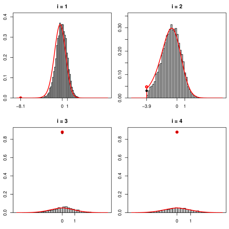
Figure 1: Adaptive Lasso, Design I: $\rho=0.3$

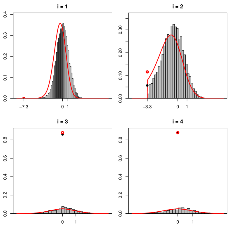
Figure 2: Adaptive Lasso, Design I: $\rho=0.5$

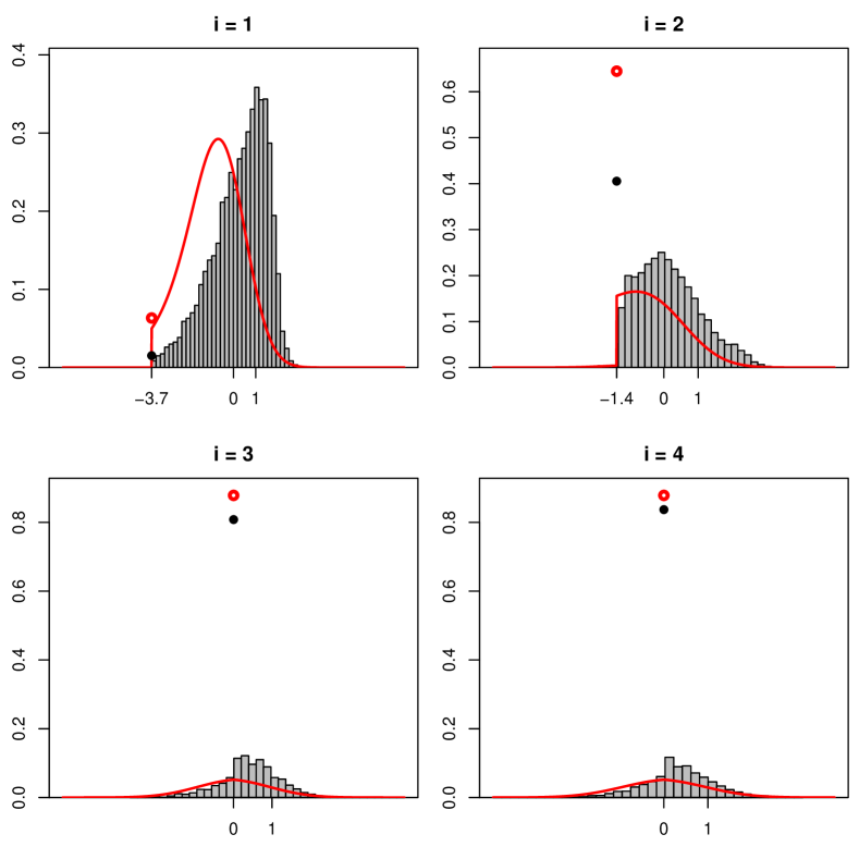
Figure 3: Adaptive Lasso, Design I: $\rho=0.9$

Figure 4: Adaptive Lasso, Design II: $c=0.2$

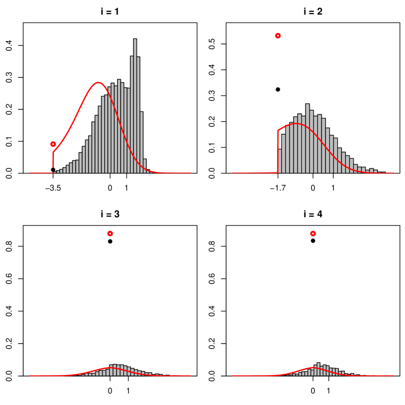
Figure 5: Adaptive Lasso, Design II: $c=2$

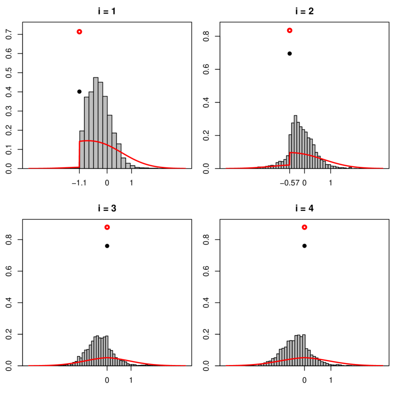
Figure 6: Adaptive Lasso, Design II: $c=-0.2$

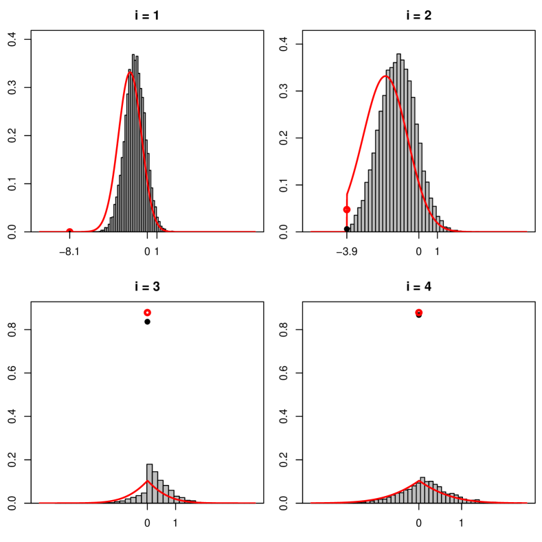
Figure 7: Lasso, Design I: $\rho=0.3$

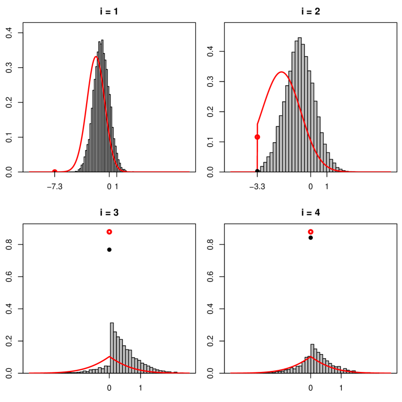
Figure 8: Lasso, Design I: $\rho=0.5$

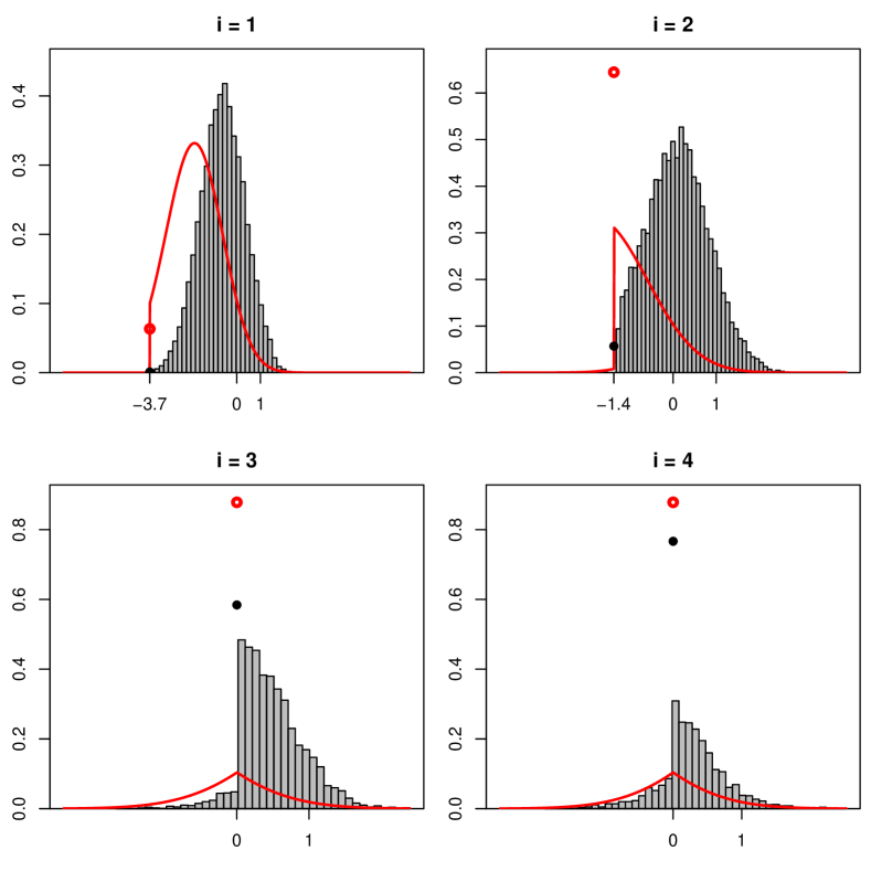
Figure 9: Lasso, Design I: $\rho=0.9$

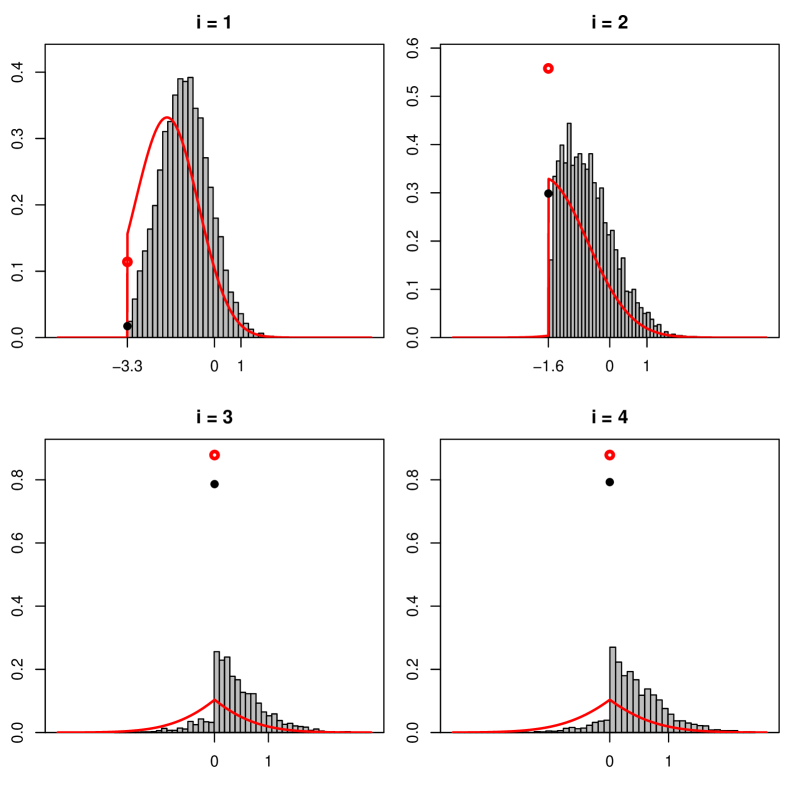
Figure 10: Lasso, Design II: $c=0.2$

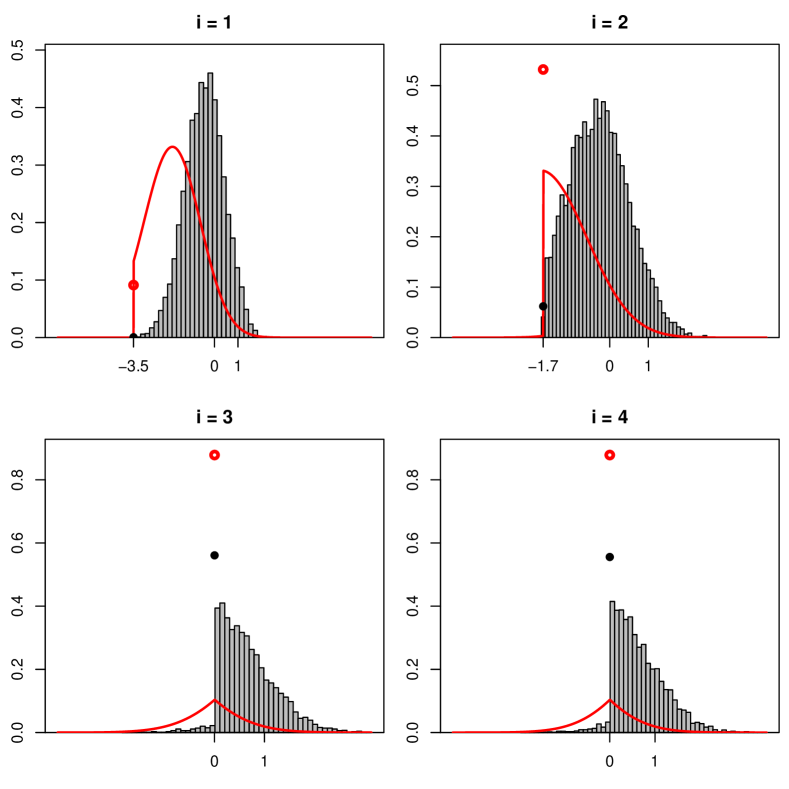
Figure 11: Lasso, Design II: $c=2$

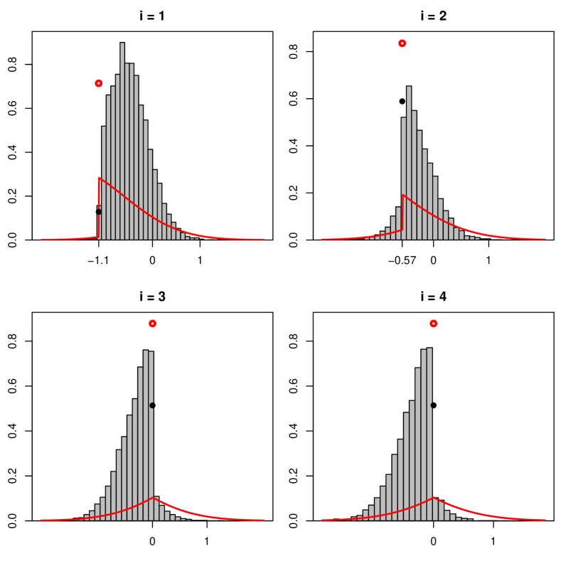
Figure 12: Lasso, Design II: $c=-0.2$

8 Proofs

8.1 Proofs for Section 3

Proof of Proposition 4: We first prove Part (a). Rewrite $P_{n,\theta,\sigma}\left(\hat{\theta}_{i}=0\right)$ as

$$\Phi\left(n^{1/2}\xi_{i,n}^{-1}\left(-\theta_{i}/\sigma+\xi_{i,n}\eta_{i,n}\right)\right)-\Phi\left(n^{1/2}\xi_{i,n}^{-1}\left(-\theta_{i}/\sigma-\xi_{i,n}\eta_{i,n}\right)\right).$$ (27)

Assume first that $\xi_{i,n}\eta_{i,n}\rightarrow 0$ and fix $\theta_{i}\neq 0$. By a standard subsequence argument we may assume without loss of generality that $n^{1/2}\xi_{i,n}^{-1}$ converges to a constant $\kappa$ which by our maintained assumption (5) must satisfy $0<\kappa\leq\infty$. Now $-\theta_{i}/\sigma\pm\xi_{i,n}\eta_{i,n}$ both converge to $-\theta_{i}/\sigma$, which is non-zero, and consequently both arguments in (27) converge to $-\kappa\theta_{i}/\sigma$. Since $\Phi$ is continuous on $\mathbb{\bar{R}}$, the expression (27) converges to zero. To prove the converse, now assume that (27) converges to zero for all $\theta_{i}\neq 0$. By a standard subsequence argument, we may assume without loss of generality that $\xi_{i,n}\eta_{i,n}$ converges to a constant $\varkappa$ satisfying $0\leq\varkappa\leq\infty$. Suppose $\varkappa>0$ holds. Choose $\theta_{i}$ such that $0<-\theta_{i}/\sigma<\varkappa$ holds. It follows that $-\theta_{i}/\sigma+\xi_{i,n}\eta_{i,n}$ and $-\theta_{i}/\sigma-\xi_{i,n}\eta_{i,n}$ eventually have opposite signs and are bounded away from zero. By our maintained assumption (5), the same is then true for the arguments in (27) leading to a contradiction. Hence $\varkappa=0$ must hold, completing the proof of Part (a). Parts (b) and (c) are obvious since $P_{n,\theta,\sigma}\left(\hat{\theta}_{i}=0\right)=\Phi\left(n^{1/2}\eta_{i,n}\right)$ $-$ $\Phi\left(-n^{1/2}\eta_{i,n}\right)$ whenever $\theta_{i}=0$. $\blacksquare$

Proof of Proposition 8: Part (a) follows immediately from (6) and the assumptions. To prove Part (b) we use (6) to write

$$P_{n,\theta^{(n)},\sigma_{n}}\left(\hat{\theta}_{i}=0\right)=\Phi\left(n^{1/2}\eta_{i,n}\left(1-\theta_{i,n}/(\sigma_{n}\xi_{i,n}\eta_{i,n})\right)\right)-\Phi\left(n^{1/2}\eta_{i,n}\left(-1-\theta_{i,n}/(\sigma_{n}\xi_{i,n}\eta_{i,n})\right)\right).$$

The first and the second claim then follow immediately. For the third claim, assume first that $\zeta_{i}=1$. Then

$$P_{n,\theta^{(n)},\sigma_{n}}\left(\hat{\theta}_{i}=0\right) =\Phi\left(n^{1/2}\left(\eta_{i,n}-\zeta_{i}\theta_{i,n}/(\sigma_{n}\xi_{i,n})\right)\right)$$

$$-\Phi\left(n^{1/2}\eta_{i,n}\left(-1-\theta_{i,n}/(\sigma_{n}\xi_{i,n}\eta_{i,n})\right)\right)\rightarrow\Phi(r_{i}).$$

The case $\zeta_{i}=-1$ is handled analogously. $\blacksquare$

Proof of Proposition 10: We prove Part (b) first. Observe that

$$P_{n,\theta,\sigma}\left(\tilde{\theta}_{i}=0\right) =\int_{0}^{\infty}\left[\Phi\left(n^{1/2}s\eta_{i,n}\right)-\Phi\left(-n^{1/2}s\eta_{i,n}\right)\right]\rho_{n-k}(s)ds$$

$$=T_{n-k}\left(n^{1/2}\eta_{i,n}\right)-T_{n-k}\left(-n^{1/2}\eta_{i,n}\right).$$

By a subsequence argument it suffices to prove the result under the assumption that $n-k=n-k(n)$ converges in $\mathbb{N}\cup\{\infty\}$. If the limit is finite, then $n-k(n)$ is eventually constant and the result follows since every $t$-distribution has unbounded support. If $n-k\rightarrow\infty$ then

$$\Phi\left(n^{1/2}\eta_{i,n}\right)-\Phi\left(-n^{1/2}\eta_{i,n}\right)-2\left\|T_{n-k}-\Phi\right\|_{\infty}$$

$$\leq P_{n,\theta,\sigma}\left(\tilde{\theta}_{i}=0\right)\leq\Phi\left(n^{1/2}\eta_{i,n}\right)-\Phi\left(-n^{1/2}\eta_{i,n}\right)+2\left\|T_{n-k}-\Phi\right\|_{\infty},$$

where $\left\|\cdot\right\|_{\infty}$ denotes the supremum norm. Since $\left\|T_{n-k}-\Phi\right\|_{\infty}\rightarrow 0$ if $n-k\rightarrow\infty$ by Polya’s Theorem, the result follows. Part (c) is proved analogously.

We next prove Part (a). Observe that the collection of distributions corresponding to $\left\{\rho_{m}:m\in\mathbb{N}\right\}$ is tight on $(0,\infty)$, meaning that for every $0<\delta<1$ there exist $0<c_{\ast}(\delta)<c^{\ast}(\delta)<\infty$ such that $\sup_{m\in\mathbb{N}}\int_{0}^{c_{\ast}(\delta)}\rho_{m}ds<\delta$ and $\sup_{m\in\mathbb{N}}\int_{c^{\ast}(\delta)}^{\infty}\rho_{m}ds<\delta$. Note that the map $s\mapsto P_{n,\theta,\sigma}\left(\hat{\theta}_{i}(s\eta_{i,n})=0\right)$ is monotonically nondecreasing. Hence,

$$\left(1-\delta\right)P_{n,\theta,\sigma}\left(\hat{\theta}_{i}(c_{\ast}(\delta)\eta_{i,n})=0\right) \leq \int_{c_{\ast}(\delta)}^{\infty}P_{n,\theta,\sigma}\left(\hat{\theta}_{i}(s\eta_{i,n})=0\right)\rho_{n-k}(s)ds$$

$$\leq P_{n,\theta,\sigma}\left(\tilde{\theta}_{i}=0\right)=\int_{0}^{\infty}P_{n,\theta,\sigma}\left(\hat{\theta}_{i}(s\eta_{i,n})=0\right)\rho_{n-k}(s)ds$$

$$\leq P_{n,\theta,\sigma}\left(\hat{\theta}_{i}(c^{\ast}(\delta)\eta_{i,n})=0\right)+\delta.$$

Since $\xi_{i,n}c_{\ast}(\delta)\eta_{i,n}$ ($\xi_{i,n}c^{\ast}(\delta)\eta_{i,n}$, respectively) converges to zero if and only if $\xi_{i,n}\eta_{i,n}$ does so, Part (a) follows from Proposition 4 applied to the estimators $\hat{\theta}_{i}(c_{\ast}(\delta)\eta_{i,n})$and $\hat{\theta}_{i}(c^{\ast}(\delta)\eta_{i,n})$. $\blacksquare$

Proof of Theorem 11: (a) Set $P_{n}(s)=P_{n,\theta^{(n)},\sigma_{n}}\left(\hat{\theta}_{i}(s\eta_{i,n})=0\right)$ for $s>0$. By Proposition 8 we have that $P_{n}(s)$ converges to $P(s)$ for all $s>0$, where $P(s)=\Phi\left(-\nu_{i}+se_{i}\right)-\Phi\left(-\nu_{i}-se_{i}\right)$ for $s>0$. Since $P_{n}(s)$ as well as $P(s)$ are continuous functions of $s$, are monotonically nondecreasing in $s$, and have the property that their limits for $s\rightarrow 0$ are $0$ while the limits for $s\rightarrow\infty$ are $1$, it follows from Polya’s Theorem that the convergence is uniform in $s$. But then using (7) gives

$$\left|P_{n,\theta^{(n)},\sigma_{n}}\left(\tilde{\theta}_{i}=0\right)-\int_{0}^{\infty}\left(\Phi\left(-\nu_{i}+se_{i}\right)-\Phi\left(-\nu_{i}-se_{i}\right)\right)\rho_{n-k}(s)ds\right|$$

$$\leq \sup_{s>0}\left|P_{n}(s)-P(s)\right|\int_{0}^{\infty}\rho_{n-k}(s)ds=\sup_{s>0}\left|P_{n}(s)-P(s)\right|\rightarrow 0$$

as $n\rightarrow\infty$. This completes the proof in case $n-k=m$ eventually; in case $n-k\rightarrow\infty$ observe that $\int_{0}^{\infty}\left(\Phi\left(-\nu_{i}+se_{i}\right)-\Phi\left(-\nu_{i}-se_{i}\right)\right)\rho_{n-k}(s)ds$ then converges to $\Phi\left(-\nu_{i}+e_{i}\right)-\Phi\left(-\nu_{i}-e_{i}\right)$ as the distribution corresponding to $\rho_{n-k}$ converges weakly to pointmass at $s=1$ and the integrand is bounded and continuous.

(b) Observe that $P_{n,\theta^{(n)},\sigma_{n}}\left(\hat{\theta}_{i}(s\eta_{i,n})=0\right)$ converges to $1$ for $s>\left|\zeta_{i}\right|$ and to $0$ for $s<\left|\zeta_{i}\right|$ by Proposition 8 applied to the estimator $\hat{\theta}_{i}(s\eta_{i,n})$. Now (7) and dominated convergence deliver the result in (b1).

Next consider (b2): Suppose first that $\left|\zeta_{i}\right|<1$. Choose $\varepsilon>0$ small enough such that $\left|\zeta_{i}\right|+\varepsilon<1$. Then, recalling that $P_{n,\theta^{(n)},\sigma_{n}}\left(\hat{\theta}_{i}(s\eta_{i,n})=0\right)$ is monotonically nondecreasing in $s$, eq. (7) gives

$$P_{n,\theta^{(n)},\sigma_{n}}\left(\tilde{\theta}_{i}=0\right) \geq \int_{\left|\zeta_{i}\right|+\varepsilon}^{\infty}P_{n,\theta^{(n)},\sigma_{n}}\left(\hat{\theta}_{i}(s\eta_{i,n})=0\right)\rho_{n-k}(s)ds$$

$$\geq P_{n,\theta^{(n)},\sigma_{n}}\left(\hat{\theta}_{i}(\left(\left|\zeta_{i}\right|+\varepsilon\right)\eta_{i,n})=0\right)\int_{\left|\zeta_{i}\right|+\varepsilon}^{\infty}\rho_{n-k}(s)ds.$$

Now the integral on the r.h.s. converges to $1$ since $\left|\zeta_{i}\right|+\varepsilon<1$, and the probability on the r.h.s. converges to $1$ by Proposition 8 applied to the estimator $\hat{\theta}_{i}(\left(\left|\zeta_{i}\right|+\varepsilon\right)\eta_{i,n})$. This completes the proof for the case $\left|\zeta_{i}\right|<1$. Next assume that $\left|\zeta_{i}\right|>1$. Choose $\varepsilon>0$ small enough such that $\left|\zeta_{i}\right|-\varepsilon>1$ holds. Then from (7) we have

$$P_{n,\theta^{(n)},\sigma_{n}}\left(\tilde{\theta}_{i}=0\right) \leq \int_{0}^{\left|\zeta_{i}\right|-\varepsilon}P_{n,\theta^{(n)},\sigma_{n}}\left(\hat{\theta}_{i}(s\eta_{i,n})=0\right)\rho_{n-k}(s)ds+\int_{\left|\zeta_{i}\right|-\varepsilon}^{\infty}\rho_{n-k}(s)ds$$

$$\leq P_{n,\theta^{(n)},\sigma_{n}}\left(\hat{\theta}_{i}(\left(\left|\zeta_{i}\right|-\varepsilon\right)\eta_{i,n})=0\right)+\int_{\left|\zeta_{i}\right|-\varepsilon}^{\infty}\rho_{n-k}(s)ds$$

since $P_{n}(s)$ is monotonically nondecreasing in $s$ and $\int_{0}^{\left|\zeta_{i}\right|-\varepsilon}\rho_{n-k}(s)ds$ is not larger than $1$. Since $\left|\zeta_{i}\right|-\varepsilon>1$ and $n-k\rightarrow\infty$ the second term on the r.h.s. goes to zero, while the first term goes to zero by Proposition 8 applied to the estimator $\hat{\theta}_{i}(\left(\left|\zeta_{i}\right|-\varepsilon\right)\eta_{i,n})$.

Next we prove 3.&4. and assume $\zeta_{i}=1$ first. Then using eq. (7) and performing the substitution $s-1=\left(2\left(n-k\right)\right)^{-1/2}t$ we obtain (recalling that $\rho_{n-k}$ is zero for negative arguments and using the abbreviations $r_{i,n}=n^{1/2}\left(\eta_{i,n}-\theta_{i,n}/(\sigma_{n}\xi_{i,n})\right)$ and $r_{i,n}^{\ast}=n^{1/2}\left(-\eta_{i,n}-\theta_{i,n}/(\sigma_{n}\xi_{i,n})\right)$)

$$P_{n,\theta^{(n)},\sigma_{n}}\left(\tilde{\theta}_{i}=0\right)$$

$$= \int_{-\infty}^{\infty}\left[\Phi\left(r_{i,n}+n^{1/2}\eta_{i,n}\left(2\left(n-k\right)\right)^{-1/2}t\right)-\Phi\left(r_{i,n}^{\ast}-n^{1/2}\eta_{i,n}\left(2\left(n-k\right)\right)^{-1/2}t\right)\right]$$

$$\times\left(2\left(n-k\right)\right)^{-1/2}\rho_{n-k}(\left(2\left(n-k\right)\right)^{-1/2}t+1)dt$$

$$= \int_{-\infty}^{\infty}\left[\Phi\left(r_{i,n}+n^{1/2}\eta_{i,n}\left(2\left(n-k\right)\right)^{-1/2}t\right)-\Phi\left(r_{i,n}^{\ast}-n^{1/2}\eta_{i,n}\left(2\left(n-k\right)\right)^{-1/2}t\right)\right]$$

$$\times\phi(t)dt+o(1).$$

The indicated term in the above display is $o(1)$ by the Lemma in the Appendix and because the expression in brackets inside the integral is bounded by $1$. Since $r_{i,n}\rightarrow r_{i}$ and $r_{i,n}^{\ast}\rightarrow-\infty$, the integrand converges to $\Phi\left(r_{i}\right)$ under 3. and to $\Phi\left(r_{i}+d_{i}t\right)$ under 4. The dominated convergence theorem then completes the proof. The case $\zeta_{i}=-1$ is treated similarly.

It remains to prove 5. Again assume $\zeta_{i}=1$ first. Define $r_{i,n}^{\prime}=2^{1/2}n^{-1/2}\eta_{i,n}^{-1}\left(n-k\right)^{1/2}r_{i,n}$ and $r_{i,n}^{\prime\prime}=2^{1/2}n^{-1/2}\eta_{i,n}^{-1}\left(n-k\right)^{1/2}r_{i,n}^{\ast}$ and rewrite the above display as

$$P_{n,\theta^{(n)},\sigma_{n}}\left(\tilde{\theta}_{i}=0\right)$$

$$= \int_{-\infty}^{\infty}\left[\Phi\left(n^{1/2}\eta_{i,n}\left(2\left(n-k\right)\right)^{-1/2}\left(r_{i,n}^{\prime}+t\right)\right)-\Phi\left(n^{1/2}\eta_{i,n}\left(2\left(n-k\right)\right)^{-1/2}\left(r_{i,n}^{\prime\prime}-t\right)\right)\right]$$

$$\times\phi(t)dt+o(1).$$

Observe that $r_{i,n}^{\prime}\rightarrow r_{i}^{\prime}$ and $r_{i,n}^{\prime\prime}\rightarrow-\infty$. The expression in brackets inside the integral hence converges to $1$ for $t>-r_{i}^{\prime}$ and to $0$ for $t<-r_{i}^{\prime}$. By dominated convergence the integral converges to $\int_{-r_{i}^{\prime}}^{\infty}\phi(t)dt=\Phi(r_{i}^{\prime})$. The case $\zeta_{i}=-1$ is treated similarly. $\blacksquare$

Proof of Proposition 13: Observe that

$$\left|P_{n,\theta,\sigma}\left(\hat{\theta}_{i}=0\right)-P_{n,\theta,\sigma}\left(\tilde{\theta}_{i}=0\right)\right|$$ (28)

$$\leq \int_{0}^{\infty}\left\{\left|\Phi\left(n^{1/2}\left(-\theta_{i}/(\sigma\xi_{i,n})+\eta_{i,n}\right)\right)-\Phi\left(n^{1/2}\left(-\theta_{i}/(\sigma\xi_{i,n})+s\eta_{i,n}\right)\right)\right|\right.$$

$$\left.+\left|\Phi\left(n^{1/2}\left(-\theta_{i}/(\sigma\xi_{i,n})-\eta_{i,n}\right)\right)-\Phi\left(n^{1/2}\left(-\theta_{i}/(\sigma\xi_{i,n})-s\eta_{i,n}\right)\right)\right|\right\}\rho_{n-k}(s)ds.$$

By a trivial modification of Lemma 13 in Pötscher and Schneider (2010) we conclude that for every $\varepsilon>0$ there exists a real number $c=c(\varepsilon)>0$ such that

$$\int_{\left|s-1\right|>(n-k)^{-1/2}c}\rho_{n-k}(s)ds<\varepsilon$$

for every $n>k$. Using the fact, that $\Phi$ is globally Lipschitz with constant $(2\pi)^{-1/2}$, this gives

$$\sup_{\theta\in\mathbb{R}^{k},0<\sigma<\infty}\left|P_{n,\theta,\sigma}\left(\hat{\theta}_{i}=0\right)-P_{n,\theta,\sigma}\left(\tilde{\theta}_{i}=0\right)\right|$$

$$\leq 2\int_{\left|s-1\right|>(n-k)^{-1/2}c}\rho_{n-k}(s)ds$$

$$+2(2\pi)^{-1/2}n^{1/2}\eta_{i,n}\int_{\left|s-1\right|\leq(n-k)^{-1/2}c}\left|s-1\right|\rho_{n-k}(s)ds$$

$$\leq 2\varepsilon+2(2\pi)^{-1/2}n^{1/2}\eta_{i,n}(n-k)^{-1/2}c$$

which proves the result since $\varepsilon$ can be made arbitrarily small. $\blacksquare$

8.2 Proofs for Section 4

Proof of Theorem 16: (a) Observe that

$$\left|\tilde{\theta}_{i}-\hat{\theta}_{LS,i}\right|\leq\hat{\sigma}\xi_{i,n}\eta_{i,n}$$ (29)

holds for any of the estimators. Hence, consistency of $\tilde{\theta}_{i}$ under $\xi_{i,n}\eta_{i,n}\rightarrow 0$ and $\xi_{i,n}/n^{1/2}\rightarrow 0$ follows immediately from Proposition 15(a) since the distributions of $\hat{\sigma}/\sigma$ are tight. Conversely, suppose $\tilde{\theta}_{i}$ is consistent. Then clearly $P_{n,\theta,\sigma}\left(\tilde{\theta}_{i}=0\right)\rightarrow 0$ whenever $\theta_{i}\neq 0$ must hold, which implies $\xi_{i,n}\eta_{i,n}\rightarrow 0$ by Proposition 10(a). This then entails consistency of $\hat{\theta}_{LS,i}$ by (29) and tightness of the distributions of $\hat{\sigma}/\sigma$; this in turn implies $\xi_{i,n}/n^{1/2}\rightarrow 0$ by Proposition 15(a).

(b) Since $a_{i,n}\rightarrow\infty$, it suffices to prove the second claim in (b). Now for every real $M>0$ we have

$$P_{n,\theta,\sigma}\left(a_{i,n}\left|\tilde{\theta}_{H,i}-\theta_{i}\right|>\sigma M\right)$$

$$= P_{n,\theta,\sigma}\left(a_{i,n}\left|\hat{\theta}_{LS,i}-\theta_{i}\right|>\sigma M,\left|\hat{\theta}_{LS,i}\right|>\hat{\sigma}\xi_{i,n}\eta_{i,n}\right)$$

$$+\boldsymbol{1}\left(a_{i,n}\left|\theta_{i}\right|>\sigma M\right)P_{n,\theta,\sigma}\left(\left|\hat{\theta}_{LS,i}\right|\leq\hat{\sigma}\xi_{i,n}\eta_{i,n}\right)$$

$$\leq P_{n,\theta,\sigma}\left(a_{i,n}\left|\hat{\theta}_{LS,i}-\theta_{i}\right|>\sigma M\right)+\boldsymbol{1}\left(a_{i,n}\left|\theta_{i}\right|>\sigma M\right)P_{n,\theta,\sigma}\left(\left|\hat{\theta}_{LS,i}\right|\leq\hat{\sigma}\xi_{i,n}\eta_{i,n}\right)$$

$$\leq P_{n,\theta,\sigma}\left(\left(n^{1/2}/\xi_{i,n}\right)\left|\hat{\theta}_{LS,i}-\theta_{i}\right|>\sigma M\right)+\boldsymbol{1}\left(a_{i,n}\left|\theta_{i}\right|>\sigma M\right)P_{n,\theta,\sigma}\left(\left|\hat{\theta}_{LS,i}\right|\leq\hat{\sigma}\xi_{i,n}\eta_{i,n}\right).$$

This gives

$$\sup_{n\in\mathbb{N}}\sup_{\theta\in\mathbb{R}^{k}}\sup_{0<\sigma<\infty}P_{n,\theta,\sigma}\left(a_{i,n}\left|\tilde{\theta}_{H,i}-\theta_{i}\right|>\sigma M\right)$$

$$\leq \sup_{n\in\mathbb{N}}\sup_{\theta\in\mathbb{R}^{k}}\sup_{0<\sigma<\infty}P_{n,\theta,\sigma}\left(\left(n^{1/2}/\xi_{i,n}\right)\left|\hat{\theta}_{LS,i}-\theta_{i}\right|>\sigma M\right)$$

$$+\sup_{n\in\mathbb{N}}\sup_{0<\sigma<\infty}\sup_{\theta\in\mathbb{R}^{k}:\left|\theta_{i}\right|>\sigma M/a_{i,n}}P_{n,\theta,\sigma}\left(\left|\hat{\theta}_{LS,i}\right|\leq\hat{\sigma}\xi_{i,n}\eta_{i,n}\right)$$

where the first term on the r.h.s. can be made arbitrarily small in view of Proposition 15(b) by choosing $M$ large enough. The second term on the r.h.s. can be written as (cf. (7))

$$\sup_{n\in\mathbb{N}}\sup_{0<\sigma<\infty}\sup_{\theta\in\mathbb{R}^{k}:\left|\theta_{i}\right|>\sigma M/a_{i,n}}\int_{0}^{\infty}P_{n,\theta,\sigma}\left(\left|\hat{\theta}_{LS,i}\right|\leq s\sigma\xi_{i,n}\eta_{i,n}\right)\rho_{n-k}(s)ds$$

$$\leq \sup_{n\in\mathbb{N}}\sup_{0<\sigma<\infty}\int_{0}^{\infty}\sup_{\theta\in\mathbb{R}^{k}:\left|\theta_{i}\right|>\sigma M/a_{i,n}}P_{n,\theta,\sigma}\left(\left|\hat{\theta}_{LS,i}\right|\leq s\sigma\xi_{i,n}\eta_{i,n}\right)\rho_{n-k}(s)ds.$$

For $\varepsilon>0$ choose $c^{\ast}(\varepsilon/2)$ as in the proof of Proposition 10. Using continuity of $\Phi$ and the fact that the probability appearing on the r.h.s. above is monotonically increasing as $\left|\theta_{i}\right|$ approaches $\sigma M/a_{i,n}$ from above, this can be further bounded by

$$\leq \sup_{n\in\mathbb{N}}\int_{0}^{\infty}\Phi\left(sn^{1/2}\eta_{i,n}-Ma_{i,n}^{-1}n^{1/2}/\xi_{i,n}\right)\rho_{n-k}(s)ds$$

$$\leq \varepsilon/2+\sup_{n\in\mathbb{N}}\int_{0}^{c^{\ast}(\varepsilon/2)}\Phi\left(sn^{1/2}\eta_{i,n}-Ma_{i,n}^{-1}n^{1/2}/\xi_{i,n}\right)\rho_{n-k}(s)ds$$

$$\leq \varepsilon/2+\sup_{n\in\mathbb{N}}\Phi\left(n^{1/2}\xi_{i,n}^{-1}a_{i,n}^{-1}\left(c^{\ast}(\varepsilon/2)\xi_{i,n}\eta_{i,n}a_{i,n}-M\right)\right)\leq\varepsilon/2+\Phi\left(c^{\ast}(\varepsilon/2)-M\right),$$

the last inequality holding for $M>c^{\ast}(\varepsilon/2)$ and since $n^{1/2}\xi_{i,n}^{-1}a_{i,n}^{-1}\geq 1$ and $\xi_{i,n}\eta_{i,n}a_{i,n}\leq 1$. Choosing $M$ sufficiently large (depending on $\varepsilon$) completes the proof for $\tilde{\theta}_{H,i}$. Next observe that

$$a_{i,n}\left|\tilde{\theta}_{H,i}-\tilde{\theta}_{S,i}\right|\leq\hat{\sigma}\min\left(n^{1/2}\eta_{i,n},1\right)\leq\hat{\sigma}$$

and similarly $a_{i,n}\left|\tilde{\theta}_{H,i}-\tilde{\theta}_{AS,i}\right|\leq\hat{\sigma}$ hold. Since the set of distributions of $\hat{\sigma}/\sigma$ (i.e., the set of distributions corresponding to $\rho_{n-k}$) is tight as already noted, this proves (b) then also for $\hat{\theta}_{S,i}$ and $\hat{\theta}_{AS,i}$.

(c) By a subsequence argument we can reduce the argument to the case where $n^{1/2}\eta_{i,n}\rightarrow e_{i}\in\mathbb{\bar{R}}$ and $n-k$ converges in $\mathbb{N}\cup\{\infty\}$. Suppose first that $e_{i}=\infty$: Observe that then $a_{i,n}=(\xi_{i,n}\eta_{i,n})^{-1}$ eventually. Choose $\theta_{i,n}$ and $\sigma_{n}$ such that $\theta_{i,n}/\left(\sigma_{n}\xi_{i,n}\eta_{i,n}\right)=\zeta_{i}$, where $\zeta_{i}$ does not depend on $n$ and $0<\left|\zeta_{i}\right|<1$ holds, and set the other coordinates of $\theta^{(n)}$ to arbitrary values (e.g., equal to zero). Observe that there exists a constant $\delta>0$ such that

$$\liminf_{n\rightarrow\infty}P_{n,\theta^{(n)},\sigma_{n}}\left(\tilde{\theta}_{i}=0\right)>\delta$$ (30)

holds: If $n-k$ converges to a finite limit, i.e., is eventually constant, the claim follows from Theorem 11(b1); if $n-k\rightarrow\infty$, then use Theorem 11(b2). By (8) we have for $\varepsilon=\delta$ and a suitable $M$ that

$$\delta > P_{n,\theta^{(n)},\sigma_{n}}\left(b_{i,n}\left|\tilde{\theta}_{i}-\theta_{i,n}\right|>\sigma_{n}M\right)\geq P_{n,\theta^{(n)},\sigma_{n}}\left(b_{i,n}\left|\tilde{\theta}_{i}-\theta_{i,n}\right|>\sigma_{n}M,\tilde{\theta}_{i}=0\right)$$

$$= P_{n,\theta^{(n)},\sigma_{n}}\left(\left|b_{i,n}\theta_{i,n}\right|/\sigma_{n}>M,\tilde{\theta}_{i}=0\right)$$

$$= \boldsymbol{1}\left(\left|b_{i,n}\theta_{i,n}\right|/\sigma_{n}>M\right)P_{n,\theta^{(n)},\sigma_{n}}\left(\tilde{\theta}_{i}=0\right)>\delta\boldsymbol{1}\left(\left|b_{i,n}\theta_{i,n}\right|/\sigma_{n}>M\right)$$

for all $n$ sufficiently large. But this is only possible if $b_{i,n}\xi_{i,n}\eta_{i,n}\leq M/\left|\zeta_{i}\right|<\infty$ holds eventually, implying that $b_{i,n}=O(a_{i,n})$. Next consider the case where $0<e_{i}<\infty$: Observe that then $a_{i,n}$ is of the same order as $n^{1/2}/\xi_{i,n}$. Then define $\theta_{i,n}$ and $\sigma_{n}$ such that $n^{1/2}\theta_{i,n}/\left(\sigma_{n}\xi_{i,n}\right)=\nu_{i}$, where $\nu_{i}$ does not depend on $n$ and $0<\left|\nu_{i}\right|<\infty$ holds, and set the other coordinates of $\theta^{(n)}$ to arbitrary values (e.g., equal to zero). Observe that then (30) also holds, in view of Theorem 11(a1) in case $n-k$ is eventually constant, and in view of Theorem 11(a2) in case $n-k\rightarrow\infty$. The rest of the proof is then similar as before. It remains to consider the case $e_{i}=0$: It follows from (29), the assumptions on $\xi_{i,n}$ and $\eta_{i,n}$, from $e_{i}=0$, and from the observation that $\hat{\theta}_{LS,i}$ is $N(\theta_{i},\sigma^{2}\xi_{i,n}^{2}/n)$-distributed, that $n^{1/2}\xi_{i,n}^{-1}\sigma^{-1}\left(\tilde{\theta}_{i}-\theta_{i}\right)$ converges in distribution to a standard normal distribution for each fixed $\theta_{i}$ and $\sigma$. Hence, stochastic boundedness of $\sigma^{-1}b_{i,n}\left|\tilde{\theta}_{i}-\theta_{i}\right|$ for each $\theta_{i}$ (and a fortiori (8)) necessarily implies that $b_{i,n}=O(n^{1/2}\xi_{i,n}^{-1})=O(a_{i,n})$.

(d) The proof for $\hat{\theta}_{i}$ is similar and in fact simpler: note that now $\left|\hat{\theta}_{i}-\hat{\theta}_{LS,i}\right|\leq\sigma\xi_{i,n}\eta_{i,n}$ holds and that in the proof of (b) the integration over $s$ can simply be replaced by evaluation at $s=1$. For (c) one uses Proposition 8 instead of Theorem 11. $\blacksquare$

8.3 Proofs for Section 5

Proofs of Propositions 19, 20, and 21: Observe that

$$\hat{\theta}_{H,i}/(\sigma\xi_{i,n})=\left(\hat{\theta}_{LS,i}/(\sigma\xi_{i,n})\right)\boldsymbol{1}\left(\left|\hat{\theta}_{LS,i}/(\sigma\xi_{i,n})\right|>\eta_{i,n}\right)$$

and that $\hat{\theta}_{LS,i}/(\sigma\xi_{i,n})$ is $N\left(\theta_{i}/(\sigma\xi_{i,n}),1/n\right)$. Furthermore, we have

$$H_{H,n,\theta,\sigma}^{i}(x) = P_{n,\theta,\sigma}\left(\sigma^{-1}\alpha_{i,n}(\hat{\theta}_{H,i}-\theta_{i})\leq x\right)$$

$$= P_{n,\theta,\sigma}\left(n^{1/2}(\hat{\theta}_{H,i}-\theta_{i})/(\sigma\xi_{i,n})\leq n^{1/2}\alpha_{i,n}^{-1}\xi_{i,n}^{-1}x\right).$$

Identifying $\hat{\theta}_{LS,i}/(\sigma\xi_{i,n})$ and $\theta_{i}/(\sigma\xi_{i,n})$ with $\bar{y}$ and $\theta$ in Pötscher and Leeb (2009) and making use of eq. (4) in that reference immediately gives the result for $dH_{H,n,\theta,\sigma}^{i}$. The result for $H_{H,n,\theta,\sigma}^{i}$ then follows from elementary calculations.

The result for $dH_{S,n,\theta,\sigma}^{i}$ follows similarly by making use of eq. (5) instead of eq. (4) in Pötscher and Leeb (2009). The result for $H_{S,n,\theta,\sigma}^{i}$ then follows from elementary calculations.

The results for $dH_{AS,n,\theta,\sigma}^{i}$ and $H_{AS,n,\theta,\sigma}^{i}$ follow similarly by making use of eqs. (9)-(11) in Pötscher and Schneider (2009). $\blacksquare$

Proofs of Propositions 23, 24, and 25: We have

$$H_{H,n,\theta,\sigma}^{i\maltese}(x) = \int_{0}^{\infty}P_{n,\theta,\sigma}\left(\sigma^{-1}\alpha_{i,n}(\tilde{\theta}_{H,i}-\theta_{i})\leq x\mid\hat{\sigma}=s\sigma\right)\rho_{n-k}(s)ds$$

$$= \int_{0}^{\infty}H_{H,s\eta_{i,n},n,\theta,\sigma}^{i}(x)\rho_{n-k}(s)ds,$$

where we have used independence of $\hat{\sigma}$ and $\hat{\theta}_{LS,i}$ allowing us to replace $\hat{\sigma}$ by $s\sigma$ in the relevant formulae, cf. Leeb and Pötscher (2003, p. 110). Substituting (9), with $\eta_{i,n}$ replaced by $s\eta_{i,n}$, into the above equation gives (23). Representing $H_{H,s\eta_{i,n},n,\theta,\sigma}^{i}(x)$ as an integral of $dH_{H,s\eta_{i,n},n,\theta,\sigma}^{i}$ given in (10) and applying Fubini’s theorem then gives (23).

Similarly, we have

$$H_{S,n,\theta,\sigma}^{i\maltese}(x)=\int_{0}^{\infty}H_{S,s\eta_{i,n},n,\theta,\sigma}^{i}(x)\rho_{n-k}(s)ds.$$

Substituting (11), with $\eta_{i,n}$ replaced by $s\eta_{i,n}$, into the above equation and noting that $\int_{0}^{\infty}\Phi(a+bs)\rho_{\nu}(s)\,ds=T_{\nu,-a}(b)$ gives (16). Elementary calculations then yield (24).

Finally, we have

$$H_{AS,n,\theta,\sigma}^{i\maltese}(x)=\int_{0}^{\infty}H_{AS,s\eta_{i,n},n,\theta,\sigma}^{i}(x)\rho_{n-k}(s)ds.$$

Substituting (13), with $\eta_{i,n}$ replaced by $s\eta_{i,n}$, into the above equation gives (18). Elementary calculations then yield (25). $\blacksquare$

8.4 Proofs for Section 6

Proof of Proposition 27 : The proof of (a) is completely analogous to the proof of Theorem 4 in Pötscher and Leeb (2009), whereas the proof of (b) is analogous to the proof of Theorem 17 in the same reference. $\blacksquare$

Proof of Proposition 28 : The proof of (a) is completely analogous to the proof of Theorem 5 in Pötscher and Leeb (2009), whereas the proof of (b) is analogous to the proof of Theorem 18 in the same reference. $\blacksquare$

Proof of Proposition 29 : The proof of (a) is completely analogous to the proof of Theorem 4 in Pötscher and Schneider (2009), whereas the proof of (b) is analogous to the proof of Theorem 6 in the same reference. $\blacksquare$

Proof of Theorem 30: Observe that the total variation distance between two cdfs is bounded by the sum of the total variation distances between the corresponding discrete and continuous parts. Furthermore, recall that the total variation distance between the absolutely continuous parts is bounded from above by the $L_{1}$-distance of the corresponding densities. Hence, from (10) and (23) we obtain

$$\left\|H_{H,n,\theta,\sigma}^{i}-H_{H,n,\theta,\sigma}^{i\maltese}\right\|_{TV}\leq A+B$$

where

$$A=\left|P_{n,\theta,\sigma}\left(\hat{\theta}_{H,i}=0\right)-P_{n,\theta,\sigma}\left(\tilde{\theta}_{H,i}=0\right)\right|$$

and

$$B = \int_{-\infty}^{\infty}\int_{0}^{\infty}\left|\boldsymbol{1}\left(\left|\alpha_{i,n}^{-1}x+\theta_{i}/\sigma\right|>\xi_{i,n}\eta_{i,n}\right)\right.$$

$$\left.-\boldsymbol{1}\left(\left|\alpha_{i,n}^{-1}x+\theta_{i}/\sigma\right|>\xi_{i,n}s\eta_{i,n}\right)\right|\rho_{n-k}(s)dsn^{1/2}\alpha_{i,n}^{-1}\xi_{i,n}^{-1}\phi\left(n^{1/2}x/(\alpha_{i,n}\xi_{i,n})\right)dx$$

$$= \int_{0}^{\infty}\int_{-\infty}^{\infty}\left|\boldsymbol{1}\left(\left|u+n^{1/2}\theta_{i}/\left(\sigma\xi_{i,n}\right)\right|>n^{1/2}\eta_{i,n}\right)\right.$$

$$\left.-\boldsymbol{1}\left(\left|u+n^{1/2}\theta_{i}/\left(\sigma\xi_{i,n}\right)\right|>sn^{1/2}\eta_{i,n}\right)\right|\phi(u)du\rho_{n-k}(s)ds$$

$$= \int_{0}^{\infty}\int_{-\infty}^{\infty}\boldsymbol{1}\left(n^{1/2}\eta_{i,n}(s\wedge 1)<\left|u+n^{1/2}\theta_{i}/(\sigma\xi_{i,n})\right|\leq n^{1/2}\eta_{i,n}(s\vee 1)\right)\phi\left(u\right)du\rho_{n-k}(s)ds$$

$$= \int_{0}^{\infty}\left\{\left[\Phi\left(n^{1/2}\left(-\theta_{i}/(\sigma\xi_{i,n})+\eta_{i,n}(s\vee 1)\right)\right)-\Phi\left(n^{1/2}\left(-\theta_{i}/(\sigma\xi_{i,n})+\eta_{i,n}(s\wedge 1)\right)\right)\right]\right.$$

$$+\left.\left[\Phi\left(n^{1/2}\left(-\theta_{i}/(\sigma\xi_{i,n})-\eta_{i,n}(s\wedge 1)\right)\right)-\Phi\left(n^{1/2}\left(-\theta_{i}/(\sigma\xi_{i,n})-\eta_{i,n}(s\vee 1)\right)\right)\right]\right\}\rho_{n-k}(s)ds,$$

where we have made use of Fubini’s theorem and performed an obvious substitution. By a trivial modification of Lemma 13 in Pötscher and Schneider (2010) we conclude that for every $\varepsilon>0$ there exists a real number $c=c(\varepsilon)>0$ such that

$$\int_{\left|s-1\right|>(n-k)^{-1/2}c}\rho_{n-k}(s)ds<\varepsilon$$ (31)

for every $n-k>0$. Using the fact, that $\Phi$ is globally Lipschitz with constant $(2\pi)^{-1/2}$, this gives

$$\sup_{\theta\in\mathbb{R}^{k},0<\sigma<\infty}B \leq 2\int_{\left|s-1\right|>(n-k)^{-1/2}c}\rho_{n-k}(s)ds$$

$$+2(2\pi)^{-1/2}n^{1/2}\eta_{i,n}\int_{\left|s-1\right|\leq(n-k)^{-1/2}c}\left|(s\vee 1)-(s\wedge 1)\right|\rho_{n-k}(s)ds$$

$$\leq 2\varepsilon+2(2\pi)^{-1/2}n^{1/2}\eta_{i,n}(n-k)^{-1/2}c.$$

The r.h.s. now converges to $2\varepsilon$ because $n^{1/2}\eta_{i,n}(n-k)^{-1/2}\rightarrow 0$. Since $\varepsilon>0$ was arbitrary, this shows that $\sup_{\theta\in\mathbb{R}^{k},0<\sigma<\infty}B$ converges to zero. Note also that $\sup_{\theta\in\mathbb{R}^{k},0<\sigma<\infty}A$ has already been shown to converge to zero in Proposition 13. This completes the proof for the hard-thresholding estimator.

With the same argument as above we obtain

$$\left\|H_{S,n,\theta,\sigma}^{i}-H_{S,n,\theta,\sigma}^{i\maltese}\right\|_{TV}\leq A+B,$$

where

$$A=\left|P_{n,\theta,\sigma}\left(\hat{\theta}_{S,i}=0\right)-P_{n,\theta,\sigma}\left(\tilde{\theta}_{S,i}=0\right)\right|$$

and

$$B = n^{1/2}\alpha_{i,n}^{-1}\xi_{i,n}^{-1}\int_{-\infty}^{\infty}\int_{0}^{\infty}\left|\phi\left(n^{1/2}x/(\alpha_{i,n}\xi_{i,n})+n^{1/2}\eta_{i,n}\right)\right.$$

$$\left.-\phi\left(n^{1/2}x/(\alpha_{i,n}\xi_{i,n})+n^{1/2}s\eta_{i,n}\right)\right|\rho_{n-k}(s)ds\boldsymbol{1}\left(\alpha_{i,n}^{-1}x+\theta_{i}/\sigma>0\right)dx$$

$$+n^{1/2}\alpha_{i,n}^{-1}\xi_{i,n}^{-1}\int_{-\infty}^{\infty}\int_{0}^{\infty}\left|\phi\left(n^{1/2}x/(\alpha_{i,n}\xi_{i,n})-n^{1/2}\eta_{i,n}\right)\right.$$

$$\left.-\phi\left(n^{1/2}x/(\alpha_{i,n}\xi_{i,n})-n^{1/2}s\eta_{i,n}\right)\right|\rho_{n-k}(s)ds\boldsymbol{1}\left(\alpha_{i,n}^{-1}x+\theta_{i}/\sigma<0\right)dx$$

where we have used (20) and (24). Now,

$$B\leq\int_{0}^{\infty}\left(B_{1}(s)+B_{2}(s)\right)\rho_{n-k}(s)ds$$

where

$$B_{1}(s) = \int_{-\infty}^{\infty}\left|\phi\left(u+n^{1/2}\eta_{i,n}\right)-\phi\left(u+n^{1/2}s\eta_{i,n}\right)\right|du,$$

$$B_{2}(s) = \int_{-\infty}^{\infty}\left|\phi\left(u-n^{1/2}\eta_{i,n}\right)-\phi\left(u-n^{1/2}s\eta_{i,n}\right)\right|du,$$

and where we have used Fubini’s theorem and an obvious substitution. It is elementary to verify that

$$B_{1}(s)=B_{2}(s)=2\left|\Phi(n^{1/2}\eta_{i,n}(s-1)/2)-\Phi(-n^{1/2}\eta_{i,n}(s-1)/2)\right|,$$

and that $B_{1}(s)\leq 2$ holds. Consequently, using (31) we obtain

$$B \leq 4\int_{\left|s-1\right|>(n-k)^{-1/2}c}\rho_{n-k}(s)ds+\int_{\left|s-1\right|\leq(n-k)^{-1/2}c}\left(B_{1}(s)+B_{2}(s)\right)\rho_{n-k}(s)ds$$

$$\leq 4\varepsilon+4(2\pi)^{-1/2}n^{1/2}\eta_{i,n}\int_{\left|s-1\right|\leq(n-k)^{-1/2}c}\left|s-1\right|\rho_{n-k}(s)ds$$

$$\leq 4\varepsilon+4(2\pi)^{-1/2}n^{1/2}\eta_{i,n}(n-k)^{-1/2}c,$$

where we have again used the fact that $\Phi$ is globally Lipschitz with constant $(2\pi)^{-1/2}$. Since $n^{1/2}\eta_{i,n}(n-k)^{-1/2}\rightarrow 0$ and $\varepsilon>0$ was arbitrary, the proof for soft-thresholding is complete, because $\sup_{\theta\in\mathbb{R}^{k},0<\sigma<\infty}A$ goes to zero by Proposition 13.

Finally, from (13) and (18) we obtain

$$\left\|H_{AS,n,\theta,\sigma}^{i}-H_{AS,n,\theta,\sigma}^{i\maltese}\right\|_{\infty} \leq \int_{0}^{\infty}\sup_{x\in\mathbb{R}}\left|\Phi\left(z_{n,\theta,\sigma}^{(2)}(x,\eta_{i,n})\right)-\Phi\left(z_{n,\theta,\sigma}^{(2)}(x,s\eta_{i,n})\right)\right|\rho_{n-k}(s)ds$$

$$+\int_{0}^{\infty}\sup_{x\in\mathbb{R}}\left|\Phi\left(z_{n,\theta,\sigma}^{(1)}(x,\eta_{i,n})\right)-\Phi\left(z_{n,\theta,\sigma}^{(1)}(x,s\eta_{i,n})\right)\right|\rho_{n-k}(s)ds$$

$$= :\int_{0}^{\infty}C_{1}(s)\rho_{n-k}(s)ds+\int_{0}^{\infty}C_{2}(s)\rho_{n-k}(s)ds.$$

Observe that on the one hand $C_{1}(s)$ and $C_{2}(s)$ are bounded by $1$, and that on the other hand, using the Lipschitz-property of $\Phi$ and the mean-value theorem,

$$\left|C_{1}(s)\right| \leq (2\pi)^{-1/2}\sup_{x\in\mathbb{R}}\left|z_{n,\theta,\sigma}^{(2)}(x,\eta_{i,n})-z_{n,\theta,\sigma}^{(2)}(x,s\eta_{i,n})\right|$$

$$= (2\pi)^{-1/2}\sup_{x\in\mathbb{R}}\left|n^{1/2}\sqrt{\left(0.5\xi_{i,n}^{-1}(\alpha_{i,n}^{-1}x+\theta_{i}/\sigma)\right)^{2}+\eta_{i,n}^{2}}\right.$$

$$\left.-n^{1/2}\sqrt{\left(0.5\xi_{i,n}^{-1}(\alpha_{i,n}^{-1}x+\theta_{i}/\sigma)\right)^{2}+s^{2}\eta_{i,n}^{2}}\right|$$

$$\leq (2\pi)^{-1/2}n^{1/2}\eta_{i,n}^{2}\left|s-1\right|\sup_{x\in\mathbb{R}}\left|\left(\left(0.5\xi_{i,n}^{-1}(\alpha_{i,n}^{-1}x+\theta_{i}/\sigma)\right)^{2}\bar{s}^{-2}+\eta_{i,n}^{2}\right)^{-1/2}\right|,$$

where $\bar{s}$ is a mean-value between $s$ and $1$ which may depend on $x$. The supremum over $x$ on the r.h.s. is now clearly assumed for $x=-\alpha_{i,n}\theta_{i}/\sigma$, resulting in the bound

$$\left|C_{1}(s)\right|\leq(2\pi)^{-1/2}n^{1/2}\eta_{i,n}\left|s-1\right|.$$

The same bound is obtained for $C_{2}$ in exactly the same way. Consequently, using (31) we obtain

$$\sup_{\theta\in\mathbb{R}^{k},0<\sigma<\infty}\left\|H_{AS,n,\theta,\sigma}^{i}-H_{AS,n,\theta,\sigma}^{i\maltese}\right\|_{\infty} \leq 2\int_{\left|s-1\right|>(n-k)^{-1/2}c}\rho_{n-k}(s)ds$$

$$+2(2\pi)^{-1/2}n^{1/2}\eta_{i,n}\int_{\left|s-1\right|\leq(n-k)^{-1/2}c}\left|s-1\right|\rho_{n-k}(s)ds$$

$$\leq 2\left[\varepsilon+(2\pi)^{-1/2}n^{1/2}\eta_{i,n}(n-k)^{-1/2}c\right].$$

Since $n^{1/2}\eta_{i,n}(n-k)^{-1/2}\rightarrow 0$ and $\varepsilon>0$ was arbitrary, the proof is complete. $\blacksquare$

Proof of Theorem 33: (a) The atomic part of $dH_{H,n,\theta^{(n)},\sigma_{n}}^{i\maltese}$ as given in (23) clearly converges weakly to the atomic part of (23) in view of Theorem 11(a1) and the fact that $\alpha_{i,n}\theta_{i,n}/\sigma_{n}=n^{1/2}\theta_{i,n}/(\sigma_{n}\xi_{i,n})\rightarrow\nu_{i}$ by assumption; also note that the atomic part converges to the zero measure in case $\left|\nu_{i}\right|=\infty$ or $e_{i}=0$ as then the total mass of the atomic part converges to zero. We turn to the absolutely continuous part next. For later use we note that what has been established so far also implies that the total mass of the absolutely continuous part converges to the total mass of the absolutely continuous part of the limit, since it is easy to see that the limiting distribution given in the theorem has total mass $1$. The density of the absolutely continuous part of (23) takes the form

$$\phi\left(x\right)\int_{0}^{\infty}\boldsymbol{1}\left(\left|x+n^{1/2}\theta_{i,n}/(\sigma_{n}\xi_{i,n})\right|>sn^{1/2}\eta_{i,n}\right)\rho_{n-k}(s)ds.$$

Observe that for given $x\in\mathbb{R}$, the indicator function in the above display converges to $\boldsymbol{1}\left(\left|x+\nu_{i}\right|>se_{i}\right)$ for Lebesgue almost all $s$. [If $e_{i}=0$, this is necessarily true only for $x\in\mathbb{R}$ with $x\neq-\nu_{i}$.] Since $n-k=m$ eventually, we get from the dominated convergence theorem that the above display converges to $\phi\left(x\right)\int_{0}^{\infty}\boldsymbol{1}\left(\left|x+\nu_{i}\right|>se_{i}\right)\rho_{m}(s)ds$ for every $x\in\mathbb{R}$ (for every $x\in\mathbb{R}$ with $x\neq-\nu_{i}$ in case $e_{i}=0$), which is the density of the absolutely continuous part in (23). Since the total mass of the absolutely continuous part is preserved in the limit as shown above, the proof is completed by Scheffé’s Lemma.

(b) Follows immediately from Proposition 27 and Theorem 30. $\blacksquare$

Proof of Theorem 34: (a) The atomic part of $dH_{S,n,\theta^{(n)},\sigma_{n}}^{i\maltese}$ as given in (24) converges weakly to the atomic part of (24) in view of Theorem 11(a1) and the fact that $\alpha_{i,n}\theta_{i,n}/\sigma_{n}=n^{1/2}\theta_{i,n}/(\sigma_{n}\xi_{i,n})\rightarrow\nu_{i}$ by assumption; also note that the atomic part converges to the zero measure in case $\left|\nu_{i}\right|=\infty$ or $e_{i}=0$ as then the total mass of the atomic part converges to zero. We turn to the absolutely continuous part next. For later use we note that what has been established so far also implies that the total mass of the absolutely continuous part converges to the total mass of the absolutely continuous part of the limit, since it is easy to see that the limiting distribution given in the theorem has total mass $1$. The density of the absolutely continuous part of (24) takes the form

$$\int_{0}^{\infty}\phi\left(x+sn^{1/2}\eta_{i,n}\right)\rho_{n-k}(s)ds\boldsymbol{1}\left(x+n^{1/2}\theta_{i,n}/(\sigma_{n}\xi_{i,n})>0\right)$$

$$+\int_{0}^{\infty}\phi\left(x-sn^{1/2}\eta_{i,n}\right)\rho_{n-k}(s)ds\boldsymbol{1}\left(x+n^{1/2}\theta_{i,n}/(\sigma_{n}\xi_{i,n})<0\right).$$

Observe that for given $x\in\mathbb{R}$, the functions $\phi\left(x\pm sn^{1/2}\eta_{i,n}\right)$ converge to $\phi\left(x\pm se_{i}\right)$, respectively, for all $s$. Since $n-k=m$ eventually, we then get from the dominated convergence theorem that the above display converges to

$$\int_{0}^{\infty}\phi\left(x+se_{i}\right)\rho_{m}(s)ds\boldsymbol{1}\left(x+\nu_{i}>0\right)+\int_{0}^{\infty}\phi\left(x-se_{i}\right)\rho_{m}(s)ds\boldsymbol{1}\left(x+\nu_{i}<0\right)$$

for every $x\mathbb{\neq-}\nu_{i}$; the last display is precisely the density of the absolutely continuous part in (24). Since the total mass of the absolutely continuous part is preserved in the limit as shown above, the proof is completed by Scheffé’s Lemma.

(b) Follows immediately from Proposition 28 and Theorem 30. $\blacksquare$

Proof of Theorem 35: (a) Observe that

$$H_{AS,n,\theta^{(n)},\sigma_{n}}^{i\maltese}(x) = \int_{0}^{\infty}\Phi\left(z_{n,\theta^{(n)},\sigma_{n}}^{(2)}(x,s\eta_{i,n})\right)\rho_{n-k}(s)ds\boldsymbol{1}\left(x+n^{1/2}\theta_{i,n}/(\sigma_{n}\xi_{i,n})\geq 0\right)$$

$$+\int_{0}^{\infty}\Phi\left(z_{n,\theta^{(n)},\sigma_{n}}^{(1)}(x,s\eta_{i,n})\right)\rho_{n-k}(s)ds\boldsymbol{1}\left(x+n^{1/2}\theta_{i,n}/(\sigma_{n}\xi_{i,n})<0\right)\,$$

where $z_{n,\theta^{(n)},\sigma_{n}}^{(1)}(x,s\eta_{i,n})$ and $z_{n,\theta^{(n)},\sigma_{n}}^{(2)}(x,s\eta_{i,n})$ reduce to

$$0.5(x-n^{1/2}\theta_{i,n}/(\sigma_{n}\xi_{i,n}))\pm\sqrt{\left(0.5(x+n^{1/2}\theta_{i,n}/(\sigma_{n}\xi_{i,n}))\right)^{2}+s^{2}n\eta_{i,n}^{2}}.$$

Clearly, $\Phi\left(z_{n,\theta^{(n)},\sigma_{n}}^{(1)}(x,s\eta_{i,n})\right)$ as well as $\Phi\left(z_{n,\theta^{(n)},\sigma_{n}}^{(2)}(x,s\eta_{i,n})\right)$ converge for every $s\geq 0$ to

$$\Phi\left(0.5(x-\nu_{i})-\sqrt{\left(0.5(x+\nu_{i})\right)^{2}+s^{2}e_{i}^{2}}\right)$$

and

$$\Phi\left(0.5(x-\nu_{i})+\sqrt{\left(0.5(x+\nu_{i})\right)^{2}+s^{2}e_{i}^{2}}\right),$$

respectively, if $\left|\nu_{i}\right|<\infty$, and the dominated convergence theorem shows that the weights of the indicator functions in (8.4) converge to the corresponding weights in (25). Since $n^{1/2}\theta_{i,n}/(\sigma_{n}\xi_{i,n})$ converges to $\nu_{i}$ by assumption, it follows that for every $x\neq-\nu_{i}$ we have convergence of $H_{AS,n,\theta^{(n)},\sigma_{n}}^{i\maltese}$ to the cdf given in (25). This proves part (a) in case $\left|\nu_{i}\right|<\infty$. In case $\nu_{i}=\infty$, we have that $z_{n,\theta^{(n)},\sigma_{n}}^{(2)}(x,s\eta_{i,n})$ converges to $x$ by an application of Proposition 15 in Pötscher and Schneider (2009). Consequently, the limit of $\Phi\left(z_{n,\theta^{(n)},\sigma_{n}}^{(2)}(x,s\eta_{i,n})\right)$ is now $\Phi\left(x\right)$. Again applying the dominated convergence theorem and observing that for each $x\in\mathbb{R}$ we have that $\boldsymbol{1}\left(x+n^{1/2}\theta_{i,n}/(\sigma_{n}\xi_{i,n})<0\right)$ is eventually zero, shows that $H_{AS,n,\theta^{(n)},\sigma_{n}}^{i\maltese}(x)$ converges to $\Phi\left(x\right)$. The case $\nu_{i}=-\infty$ is proved analogously.

(b) Follows immediately from Proposition 29 and Theorem 30. $\blacksquare$

Proof of Theorem 36: Observe that

$$\sigma_{n}^{-1}\alpha_{i,n}(\tilde{\theta}_{H,i}-\theta_{i,n}) = -\theta_{i,n}/(\sigma_{n}\xi_{i,n}\eta_{i,n})\boldsymbol{1}\left(\tilde{\theta}_{H,i}=0\right)$$

$$+(\sigma_{n}\xi_{i,n}\eta_{i,n})^{-1}\left(\hat{\theta}_{LS,i}-\theta_{i,n}\right)\boldsymbol{1}\left(\tilde{\theta}_{H,i}\neq 0\right)$$

$$= -\theta_{i,n}/(\sigma_{n}\xi_{i,n}\eta_{i,n})\boldsymbol{1}\left(\tilde{\theta}_{H,i}=0\right)+n^{-1/2}\eta_{i,n}^{-1}Z_{n}\boldsymbol{1}\left(\tilde{\theta}_{H,i}\neq 0\right)$$

where $Z_{n}$ is standard normally distributed. The expressions in front of the indicator functions now converge to $-\zeta_{i}$ and $0$, respectively, in probability as $n\rightarrow\infty$. Inspection of the cdf of $\sigma_{n}^{-1}\alpha_{i,n}(\tilde{\theta}_{H,i}-\theta_{i,n})$ then shows that this cdf converges weakly to

$$\left(\lim_{n\rightarrow\infty}P_{n,\theta^{(n)},\sigma_{n}}\left(\tilde{\theta}_{H,i}=0\right)\right)\delta_{-\zeta_{i}}+\left(1-\lim_{n\rightarrow\infty}P_{n,\theta^{(n)},\sigma_{n}}\left(\tilde{\theta}_{H,i}=0\right)\right)\delta_{0}$$

if $\left|\zeta_{i}\right|<\infty$. Part (b) of Theorem 11 completes the proof of both parts of the theorem in case $\left|\zeta_{i}\right|<\infty$. If $\left|\zeta_{i}\right|=\infty$ the same theorem shows that the weak limit is now $\delta_{0}$. $\blacksquare$

Proof of Theorem 37: (a) The atomic part of $dH_{S,n,\theta^{(n)},\sigma_{n}}^{i\maltese}$ as given in (24) converges weakly to the atomic part given in (26) by Theorem 11(b1). The density of the absolutely continuous part of $dH_{S,n,\theta^{(n)},\sigma_{n}}^{i\maltese}$ can be written as

$$n^{1/2}\eta_{i,n}\int_{-\infty}^{\infty}\phi\left(n^{1/2}\eta_{i,n}\left(x+s\right)\right)\rho_{m}(s)ds\boldsymbol{1}\left(x+\theta_{i,n}/(\sigma_{n}\xi_{i,n}\eta_{i,n})>0\right)$$

$$+n^{1/2}\eta_{i,n}\int_{-\infty}^{\infty}\phi\left(n^{1/2}\eta_{i,n}\left(x-s\right)\right)\rho_{m}(s)ds\boldsymbol{1}\left(x+\theta_{i,n}/(\sigma_{n}\xi_{i,n}\eta_{i,n})<0\right)$$

recalling the convention that $\rho_{m}(s)=0$ for $s<0$. Note that with this convention $\rho_{m}$ is then a bounded continuous function on the real line. Since $n^{1/2}\eta_{i,n}\phi\left(n^{1/2}\eta_{i,n}\left(x+\cdot\right)\right)$ and $n^{1/2}\eta_{i,n}\phi\left(n^{1/2}\eta_{i,n}\left(x-\cdot\right)\right)$ clearly converge weakly to $\delta_{-x}$ and $\delta_{x}$, respectively, the density of the absolutely continuous part of $dH_{S,n,\theta^{(n)},\sigma_{n}}^{i\maltese}$ is seen to converge to $\rho_{m}(-x)\boldsymbol{1}\left(x+\zeta_{i}>0\right)+\rho_{m}(x)\boldsymbol{1}\left(x+\zeta_{i}<0\right)$ for every $x\neq-\zeta_{i}$. An application of Scheffé’s Lemma then completes the proof, noting that the total mass of the absolutely continuous part of $dH_{S,n,\theta^{(n)},\sigma_{n}}^{i\maltese}$ converges to the total mass of the absolutely continuous part of (26) as the same is true for the atomic part in view of Theorem 11(b1) (and since the distributions involved all have total mass $1$).

(b) Rewrite $\sigma_{n}^{-1}\alpha_{i,n}(\tilde{\theta}_{S,i}-\theta_{i,n})$ as

$$-\theta_{i,n}/(\sigma_{n}\xi_{i,n}\eta_{i,n})\boldsymbol{1}\left(\tilde{\theta}_{S,i}=0\right)+\left(W_{n}-\left(\hat{\sigma}/\sigma_{n}\right)\mathop{\mathrm{s}ign}(W_{n}+\theta_{i,n}/(\sigma_{n}\xi_{i,n}\eta_{i,n}))\right)\boldsymbol{1}\left(\tilde{\theta}_{S,i}\neq 0\right),$$

where $W_{n}$ is a sequence of $N(0,n^{-1}\eta_{i,n}^{-2})$-distributed random variables. Observe that $\theta_{i,n}/(\sigma_{n}\xi_{i,n}\eta_{i,n})$ converges to $\zeta_{i}$ and that $W_{n}$ converges to zero in $P_{n,\theta^{(n)},\sigma_{n}}$-probability. Now, if $\left|\zeta_{i}\right|<1$, then $P_{n,\theta^{(n)},\sigma_{n}}\left(\tilde{\theta}_{S,i}=0\right)\rightarrow 1$ by Theorem 11(b2), and hence $\sigma_{n}^{-1}\alpha_{i,n}(\tilde{\theta}_{S,i}-\theta_{i,n})$ converges to $-\zeta_{i}$ in $P_{n,\theta^{(n)},\sigma_{n}}$-probability. This proves the result in case $\left|\zeta_{i}\right|<1$. In case $\left|\zeta_{i}\right|>1$ we have that

$$P_{n,\theta^{(n)},\sigma_{n}}\left(\tilde{\theta}_{S,i}\neq 0\right)\rightarrow 1$$

and

$$P_{n,\theta^{(n)},\sigma_{n}}\left(\mathop{\mathrm{s}ign}(W_{n}+\theta_{i,n}/(\sigma_{n}\xi_{i,n}\eta_{i,n}))=\mathop{\mathrm{s}ign}(\zeta_{i})\right)\rightarrow 1.$$ (33)

Clearly, also $\hat{\sigma}/\sigma_{n}$ converges to $1$ in $P_{n,\theta^{(n)},\sigma_{n}}$-probability since $n-k\rightarrow\infty$. Consequently, $\sigma_{n}^{-1}\alpha_{i,n}(\tilde{\theta}_{S,i}-\theta_{i,n})$ converges to $-\mathop{\mathrm{s}ign}(\zeta_{i})$ in $P_{n,\theta^{(n)},\sigma_{n}}$-probability, which proves the case $\left|\zeta_{i}\right|>1$. Finally, if $\left|\zeta_{i}\right|=1$, then (33) continues to hold and we can write

$$\sigma_{n}^{-1}\alpha_{i,n}(\tilde{\theta}_{S,i}-\theta_{i,n}) = \left(-\zeta_{i}+o(1)\right)\boldsymbol{1}\left(\tilde{\theta}_{S,i}=0\right)-\left(o_{p}(1)+\left(1+o_{p}(1)\right)\mathop{\mathrm{s}ign}(\zeta_{i})\right)\boldsymbol{1}\left(\tilde{\theta}_{S,i}\neq 0\right)$$

$$= -\mathop{\mathrm{s}ign}(\zeta_{i})+o_{p}(1),$$

where $o_{p}(1)$ refers to a term that converges to zero in $P_{n,\theta^{(n)},\sigma_{n}}$-probability. This then completes the proof of part (b). $\blacksquare$

Proof of Theorem 38: (a) Assume first that $0\leq\zeta_{i}<\infty$ holds. Note that $z_{n,\theta^{(n)},\sigma_{n}}^{(1)}(x,s\eta_{i,n})$ and $z_{n,\theta^{(n)},\sigma_{n}}^{(2)}(x,s\eta_{i,n})$ now reduce to

$$n^{1/2}\eta_{i,n}\left[0.5(x-\theta_{i,n}/(\sigma_{n}\xi_{i,n}\eta_{i,n}))\pm\sqrt{\left(0.5(x+\theta_{i,n}/(\sigma_{n}\xi_{i,n}\eta_{i,n}))\right)^{2}+s^{2}}\right].$$

First, for $x>-\zeta_{i}$ we see that $H_{AS,n,\theta^{(n)},\sigma_{n}}^{i\maltese}(x)$ eventually reduces to

$$\int_{0}^{\infty}\Phi\left(z_{n,\theta^{(n)},\sigma_{n}}^{(2)}(x,s\eta_{i,n})\right)\rho_{m}(s)ds.$$

Furthermore, for $x\geq 0$ we see that $z_{n,\theta^{(n)},\sigma_{n}}^{(2)}(x,s\eta_{i,n})\rightarrow\infty$ for all $s>0$ whereas for $-\zeta_{i}<x<0$ we have that $z_{n,\theta^{(n)},\sigma_{n}}^{(2)}(x,s\eta_{i,n})\rightarrow\infty$ for $s>\sqrt{-x\zeta_{i}}$ and $z_{n,\theta^{(n)},\sigma_{n}}^{(2)}(x,s\eta_{i,n})\rightarrow-\infty$ for $s<\sqrt{-x\zeta_{i}}$. As a consequence, we obtain from the dominated convergence theorem that $H_{AS,n,\theta^{(n)},\sigma_{n}}^{i\maltese}(x)$ converges to $1$ for $x\geq 0$ and to $\int_{\sqrt{-x\zeta_{i}}}^{\infty}\rho_{m}(s)ds$ for $-\zeta_{i}<x<0$. Second, for $x<-\zeta_{i}$ note that $H_{AS,n,\theta^{(n)},\sigma_{n}}^{i\maltese}(x)$ eventually reduces to

$$\int_{0}^{\infty}\Phi\left(z_{n,\theta^{(n)},\sigma_{n}}^{(1)}(x,s\eta_{i,n})\right)\rho_{m}(s)ds$$

and that $z_{n,\theta^{(n)},\sigma_{n}}^{(1)}(x,s\eta_{i,n})\rightarrow-\infty$ for all $s>0$ in this case. This shows that for $x<-\zeta_{i}$ we have that $H_{AS,n,\theta^{(n)},\sigma_{n}}^{i\maltese}(x)$ converges to $0$. But this proves the result for the case $0\leq\zeta_{i}<\infty$. In case $\zeta_{i}=\infty$ the same reasoning shows that now $H_{AS,n,\theta^{(n)},\sigma_{n}}^{i\maltese}(x)$ eventually reduces to

$$\int_{0}^{\infty}\Phi\left(z_{n,\theta^{(n)},\sigma_{n}}^{(2)}(x,s\eta_{i,n})\right)\rho_{m}(s)ds$$

for all $x$, and that now for $x>0$ we have $z_{n,\theta^{(n)},\sigma_{n}}^{(2)}(x,s\eta_{i,n})\rightarrow\infty$ for all $s>0$ whereas for $x<0$ we have that $z_{n,\theta^{(n)},\sigma_{n}}^{(2)}(x,s\eta_{i,n})\rightarrow-\infty$ for all $s>0$. This shows that $H_{AS,n,\theta^{(n)},\sigma_{n}}^{i\maltese}$ converges weakly to $\delta_{0}$ in case $\zeta_{i}=\infty$. The proof for the case $\zeta_{i}<0$ is completely analogous.

(b) Rewrite $\sigma_{n}^{-1}\alpha_{i,n}(\tilde{\theta}_{AS,i}-\theta_{i,n})$ as

$$-\theta_{i,n}/(\sigma_{n}\xi_{i,n}\eta_{i,n})\boldsymbol{1}\left(\tilde{\theta}_{AS,i}=0\right)$$

$$+\left(\sigma_{n}\xi_{i,n}\eta_{i,n}\right)^{-1}\left(\hat{\theta}_{LS,i}-\theta_{i,n}-\hat{\sigma}^{2}\xi_{i,n}^{2}\eta_{i,n}^{2}/\hat{\theta}_{LS,i}\right)\boldsymbol{1}\left(\tilde{\theta}_{AS,i}\neq 0\right)$$

$$= -\theta_{i,n}/(\sigma_{n}\xi_{i,n}\eta_{i,n})\boldsymbol{1}\left(\tilde{\theta}_{AS,i}=0\right)+\left(W_{n}-\left(\hat{\sigma}^{2}/\sigma_{n}\right)\xi_{i,n}\eta_{i,n}/\hat{\theta}_{LS,i}\right)\boldsymbol{1}\left(\tilde{\theta}_{AS,i}\neq 0\right)$$

$$= -\theta_{i,n}/(\sigma_{n}\xi_{i,n}\eta_{i,n})\boldsymbol{1}\left(\tilde{\theta}_{AS,i}=0\right)$$

$$+\left(W_{n}-\left(\hat{\sigma}^{2}/\sigma_{n}^{2}\right)\left(W_{n}+\theta_{i,n}/(\sigma_{n}\xi_{i,n}\eta_{i,n})\right)^{-1}\right)\boldsymbol{1}\left(\tilde{\theta}_{AS,i}\neq 0\right)$$

where $W_{n}$ is a sequence of $N(0,n^{-1}\eta_{i,n}^{-2})$-distributed random variables. Note that $\theta_{i,n}/(\sigma_{n}\xi_{i,n}\eta_{i,n})$ converges to $\zeta_{i}$ by assumption. Now, if $\left|\zeta_{i}\right|<1$, then $P_{n,\theta^{(n)},\sigma_{n}}\left(\tilde{\theta}_{AS,i}=0\right)\rightarrow 1$ by Theorem 11(b2), hence $\sigma_{n}^{-1}\alpha_{i,n}(\tilde{\theta}_{AS,i}-\theta_{i,n})$ converges to $-\zeta_{i}$ in $P_{n,\theta^{(n)},\sigma_{n}}$-probability, establishing the result in this case. Furthermore, for $1\leq\left|\zeta_{i}\right|\leq\infty$ rewrite the above display as

$$\left(-\zeta_{i}+o(1)\right)\boldsymbol{1}\left(\tilde{\theta}_{AS,i}=0\right)+\left(o_{p}(1)-\left(1+o_{p}(1)\right)\left(\zeta_{i}+o_{p}(1)\right)^{-1}\right)\boldsymbol{1}\left(\tilde{\theta}_{AS,i}\neq 0\right)$$

$$= \left(-\zeta_{i}+o(1)\right)\boldsymbol{1}\left(\tilde{\theta}_{AS,i}=0\right)+\left(-\zeta_{i}^{-1}+o_{p}(1)\right)\boldsymbol{1}\left(\tilde{\theta}_{AS,i}\neq 0\right),$$

with the convention that $\zeta_{i}^{-1}=0$ in case $\left|\zeta_{i}\right|=\infty$. If $\left|\zeta_{i}\right|>1$ (including the case $\left|\zeta_{i}\right|=\infty$) then $P_{n,\theta^{(n)},\sigma_{n}}\left(\tilde{\theta}_{AS,i}\neq 0\right)\rightarrow 1$ by Theorem 11(b2), and hence the last display shows that $\sigma_{n}^{-1}\alpha_{i,n}(\tilde{\theta}_{AS,i}-\theta_{i,n})$ converges to $-\zeta_{i}^{-1}$ in $P_{n,\theta^{(n)},\sigma_{n}}$-probability, establishing the result in this case. Finally, if $\left|\zeta_{i}\right|=1$ holds, then the last line in the above display reduces to $-\zeta_{i}+o_{p}(1)$, completing the proof of part (b). $\blacksquare$

Proof of Proposition 39: (a) By a subsequence argument we may assume that $n-k$ converges in $\mathbb{N\cup\{\infty\}}$. Applying Theorem 11(b) we obtain that $P_{n,\theta,\sigma}\left(\tilde{\theta}_{H,i}=0\right)$ converges to $1$ in case $\theta_{i}=0$, and to $0$ in case $\theta_{i}\neq 0$. Observe that

$$\sigma^{-1}n^{1/2}\xi_{i,n}^{-1}\left(\tilde{\theta}_{H,i}-\theta_{i}\right)=-\sigma^{-1}n^{1/2}\xi_{i,n}^{-1}\theta_{i}$$

holds on the event $\tilde{\theta}_{H,i}=0$, while

$$\sigma^{-1}n^{1/2}\xi_{i,n}^{-1}\left(\tilde{\theta}_{H,i}-\theta_{i}\right)=\sigma^{-1}n^{1/2}\xi_{i,n}^{-1}\left(\hat{\theta}_{LS,i}-\theta_{i}\right)=:Z_{n}$$

holds on the event $\tilde{\theta}_{H,i}\neq 0$. The result then follows in view of the fact that $Z_{n}$ is standard normally distributed. The proof for $\hat{\theta}_{H,i}$ is similar using Proposition 8(b) instead of Theorem 11(b) (it is in fact simpler as the subsequence argument is not needed).

(b) Again we may assume that $n-k$ converges in $\mathbb{N\cup\{\infty\}}$. By the same reference as in the proof of (a) we obtain that $P_{n,\theta,\sigma}\left(\tilde{\theta}_{AS,i}=0\right)$ converges to $1$ in case $\theta_{i}=0$, and to $0$ in case $\theta_{i}\neq 0$. Now

$$\sigma^{-1}n^{1/2}\xi_{i,n}^{-1}\left(\tilde{\theta}_{AS,i}-\theta_{i}\right)=-\sigma^{-1}n^{1/2}\xi_{i,n}^{-1}\theta_{i}$$

holds on the event $\tilde{\theta}_{AS,i}=0$ and the claim for $\theta_{i}=0$ follows immediately. On the event $\tilde{\theta}_{AS,i}\neq 0$ we have from the definition of the estimator

$$\sigma^{-1}n^{1/2}\xi_{i,n}^{-1}\left(\tilde{\theta}_{AS,i}-\theta_{i}\right) = \sigma^{-1}n^{1/2}\xi_{i,n}^{-1}\left(\hat{\theta}_{LS,i}-\theta_{i}-\hat{\sigma}^{2}\xi_{i,n}^{2}\eta_{i,n}^{2}/\hat{\theta}_{LS,i}\right)$$

$$= Z_{n}-\left(\hat{\sigma}/\sigma\right)^{2}\left(\left(n\eta_{i,n}^{2}\right)^{-1}Z_{n}+\sigma^{-1}\xi_{i,n}^{-1}n^{-1/2}\eta_{i,n}^{-2}\theta_{i}\right)^{-1}.$$

Now, if $\theta_{i}\neq 0$, then the event $\tilde{\theta}_{AS,i}\neq 0$ has probability approaching $1$ as shown above. Hence, we have on events that have probability tending to $1$

$$\sigma^{-1}n^{1/2}\xi_{i,n}^{-1}\left(\tilde{\theta}_{AS,i}-\theta_{i}\right) = Z_{n}-\left(\hat{\sigma}/\sigma\right)^{2}\left(o_{p}(1)+\sigma^{-1}\xi_{i,n}^{-1}n^{-1/2}\eta_{i,n}^{-2}\theta_{i}\right)^{-1}$$

$$= Z_{n}-o_{p}(1),$$

since $n\eta_{i,n}^{2}\rightarrow\infty$ and $\xi_{i,n}^{-1}n^{-1/2}\eta_{i,n}^{-2}\rightarrow\infty$ by the assumption and since $\theta_{i}\neq 0$; also note that $\hat{\sigma}/\sigma$ is stochastically bounded since the collection of distributions corresponding to $\rho_{m}$ with $m\in\mathbb{N}$ is tight on $(0,\infty)$ as was noted earlier. The proof for $\hat{\theta}_{AS,i}$ is again similar (and simpler) by using Proposition 8(b) instead of Theorem 11(b). $\blacksquare$

9 References

Alliney, S. & S. A. Ruzinsky (1994): An algorithm for the minimization of mixed $l_{1}$ and $l_{2}$ norms with applications to Bayesian estimation. IEEE Transactions on Signal Processing  42, 618-627.

Bauer, P., Pötscher, B. M. & P. Hackl (1988): Model selection by multiple test procedures. Statistics  19, 39–44.

Donoho, D. L., Johnstone, I. M., Kerkyacharian, G., D. Picard (1995): Wavelet shrinkage: asymptopia? With discussion and a reply by the authors. Journal of the Royal Statistical Society Series B  57, 301–369.

Fan, J. & R. Li (2001): Variable selection via nonconcave penalized likelihood and its oracle properties. Journal of the American Statistical Association  96, 1348-1360.

Fan, J. & H. Peng (2004): Nonconcave penalized likelihood with a diverging number of parameters. Annals of Statistics  32, 928–961.

Feller, W. (1957): An Introduction to Probability Theory and Its Applications, Volume 1. 2nd ed., Wiley, New York.

Frank, I. E. & J. H. Friedman (1993): A statistical view of some chemometrics regression tools (with discussion). Technometrics  35, 109-148.

Ibragimov, I. A. (1956): On the composition of unimodal distributions. Theory of Probability and its Applications  1, 255-260.

Knight, K. & W. Fu (2000): Asymptotics for lasso-type estimators. Annals of Statistics  28, 1356-1378.

Leeb, H. & B. M. Pötscher (2003): The finite-sample distribution of post-model-selection estimators and uniform versus nonuniform approximations. Econometric Theory  19, 100–142.

Leeb, H. & B. M. Pötscher (2005): Model selection and inference: facts and fiction. Econometric Theory  21, 21–59.

Leeb, H. & B. M. Pötscher (2008): Sparse estimators and the oracle property, or the return of Hodges’ estimator. Journal of Econometrics  142, 201-211.

Pötscher, B. M. (1991): Effects of model selection on inference. Econometric Theory  7, 163–185.

Pötscher, B. M. (2006): The distribution of model averaging estimators and an impossibility result regarding its estimation. IMS Lecture Notes-Monograph Series  52, 113–129.

Pötscher, B. M. & H. Leeb (2009): On the distribution of penalized maximum likelihood estimators: the LASSO, SCAD, and thresholding. Journal of Multivariate Analysis  100, 2065-2082.

Pötscher, B. M. & U. Schneider (2009): On the distribution of the adaptive LASSO estimator. Journal of Statistical Planning and Inference  139, 2775-2790.

Pötscher, B. M. & U. Schneider (2010): Confidence sets based on penalized maximum likelihood estimators in Gaussian regression. Electronic Journal of Statistics  10, 334-360.

Sen, P. K. (1979): Asymptotic properties of maximum likelihood estimators based on conditional specification. Annals of Statistics  7, 1019-1033.

Tibshirani, R. (1996): Regression shrinkage and selection via the lasso. Journal of the Royal Statistical Society Series B  58, 267-288.

Zhang, C.-H. (2010): Nearly unbiased variable selection under minimax concave penalty. Annals of Statistics  38, 894-942.

Zou, H. (2006): The adaptive lasso and its oracle properties. Journal of the American Statistical Association  101, 1418-1429.

Appendix A Appendix

Recall that $\rho_{m}(x)=0$ for $x<0$.

Lemma 46

$(2m)^{-1/2}\rho_{m}((2m)^{-1/2}t+1)$ converges to $\phi(t)$ in the $L_{1}$-sense as $m\rightarrow\infty$.

Proof. Observe that $(2m)^{-1/2}\rho_{m}((2m)^{-1/2}t+1)$ is the density of $U_{m}=(2m)^{1/2}\left(\sqrt{\chi_{m}^{2}/m}-1\right)$ where $\chi_{m}^{2}$ denotes a chi-square distributed random variable with $m$ degrees of freedom. By the central limit theorem and the delta-method $U_{m}$ converges in distribution to a standard normal random variable. With

$$g_{m}(x)=2^{-m/2}\left(\Gamma(m/2)\right)^{-1}x^{(m/2)-1}\exp(-x/2)\qquad\text{for }x>0$$

being the density of $\chi_{m}^{2}$ we have for $x>0$

$$\rho_{m}(x) = 2mxg_{m}(mx^{2})=2^{1-m/2}\left(\Gamma(m/2)\right)^{-1}m^{1/2}\left(mx^{2}\right)^{(m/2)-1/2}\exp\left(-mx^{2}/2\right)$$

$$= (8m)^{1/2}\Gamma(\left(m+1\right)/2)\left(\Gamma(m/2)\right)^{-1}g_{m+1}\left(mx^{2}\right).$$

and we have $\rho_{m}(x)=0$ for $x\leq 0$. Since the cdf associated with $g_{m+1}$ is unimodal, this shows that the same is true for the cdf associated with $\rho_{m}$. But then convergence in distribution of $U_{m}$ implies convergence of $m^{-1/2}\rho_{m}(m^{-1/2}t+1)$ to $\phi(t)$ in the $L_{1}$-sense by a result of Ibragimov (1956), Scheffé’s Lemma, and a standard subsequence argument.