Closed form solution for a double quantum well using Gröbner basis

Abstract

Analytical expressions for spectrum, eigenfunctions and dipole matrix elements of a square double quantum well (DQW) are presented for a general case when the potential in different regions of the DQW has different heights and effective masses are different. This was achieved by Gröbner basis algorithm which allows to disentangle the resulting coupled polynomials without explicitly solving the transcendental eigenvalue equation.

Keywords: Heterostructures, Double quantum well, Eigenfunctions, Gröbner basis, Optical dipole matrix element, Closed form solution

1 Introduction

The square double quantum well (DQW) often is used as a toy model to demonstrate the interaction between quantized energy levels due to particle tunneling through a potential barrier separating individual wells [1, 2, 3, 4, 5, 6]. Recently the DQW model had attracted considerable attention in semiconductor heterostructure physics because of its applications in nanoelectronics [7, 8, 9]. The tunneling conductance properties of semiconducting DQW devices as well as drag effects that result from interaction between electrons moving at different velocities in different wells was recently discussed, for example, in review articles [10, 11].

Appearance of transcendental equations that describe DQW spectrum limits direct application of analytical methods in tackling the eigenfunction problems. Initially the problem of finding the eigenfunctions has been solved by perturbation theory assuming that energy level splitting due to tunneling is small [1]. The most recent analytical approach heavily relies on symmetry properties of the DQW [6]. Of course, this restriction can be relaxed by resorting to numerical methods [2, 4, 6, 8, 12]. However, in many cases a knowledge of analytical form of the wave function is more preferable. For example, in the wave packet dynamics problems the closed form solution allows one to construct a direct superposition of eigenfunctions to make a computational task easy. Here we demonstrate that one can push the problem further and calculate the relevant eigenfunctions exactly by exploiting a computer based Gröbner basis algorithm [13]. In sections 2 and 3 the spectrum and eigenfunctions of a general DQW are calculated using the Gröbner basis, and in section 4 the results are applied to find closed form expression for optical dipole matrix element of the DQW.

2 Spectrum

The one-dimensional DQW with flat potentials in each of regions $1-5$, as shown in figure 1, is described by the following piecewise function of coordinate $x$

$$V(x)=\cases{V_{c}&if $x<0$\\ 0&if $0\leq x\leq a$\\ V_{b}&if $a<x<a+b$\\ 0&if $a+b\leq x\leq 2a+b$\\ V_{c}&if $x>2a+b$\\ },$$ (2.1)

where $V_{c}$ is the confining potential (referenced from the bottom of wells) and $V_{b}$ is the height of central barrier separating two identical quantum wells. The mirror symmetry of the system ensures that the quantum states of such a DQW have either even or odd parity.

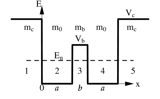
Figure 1: Symmetric double quantum well with central barrier of width $b$ and height $V_{b}$. The eigenenergy $E_{n}$ is referenced from the bottom of wells of width $a$. Electron effective mass in regions $1-5$ is assumed to be different.

Only bound states will be considered here. These states can be normalized to unity over entire $x$ axis. The wave function $\psi(x)$ in the regions $1-5$ has the following shapes:

$$\eqalign{\psi_{1}=&B_{1}\rme^{\chi_{c}x},\\ \psi_{2}=&A_{1}\sin kx+C_{1}\cos kx,\\ \psi_{3}=&B_{2}\rme^{\chi_{b}(a-x)}+B_{3}\rme^{-\chi_{b}(a+b-x)},\\ \psi_{4}=&A_{2}\sin k(2a+b-x)+C_{2}\cos k(2a+b-x),\\ \psi_{5}=&B_{4}\rme^{\chi_{c}(2a+b-x)},}$$ (2.2)

where $k$ is the free-electron wave vector, $k=\sqrt{2m_{0}E/\hbar^{2}}$, in the quantum wells of width $a$. The energy $E$ is referenced from the bottom of the wells. The wave vectors of evanescent waves in the exponents are $\chi_{b}=\sqrt{(2m_{b}/\hbar^{2})(V_{b}-E)}$ and $\chi_{c}=\sqrt{(2m_{c}/\hbar^{2})(V_{c}-E)}$, where we have introduced different electron masses, namely, $m_{0}$ inside the wells, $m_{b}$ in the barrier and $m_{c}$ in the confining potential. This is typical to semiconductor heterostructures, where the DQW is made of nanometer layers having different forbidden energy gaps. As a result, the electron effective mass depends on coordinate $x$.

In equations (2.2) there are eight unknown coefficients that must be calculated. Because of symmetry, the number of coefficients, in fact, can be reduced. However we shall not do this since the Gröbner basis algorithm will take account of symmetry properties of polynomials automatically. The standard BenDaniel-Duke boundary condition [14] which takes into account mass difference on right ($r$) and left ($l$) sides of the potential step at coordinates $X=0$, $X=a$, $X=a+b$ and $X=2a+b$ will be used

$$\psi_{r}(X^{+}) =\psi_{l}(X^{-})\,,$$ (2.3a)

$$\frac{1}{m_{r}}\frac{\partial\psi_{r}}{\partial x}\Big{|}_{X^{+}} =\frac{1}{m_{l}}\frac{\partial\psi_{l}}{\partial x}\Big{|}_{X^{-}}.$$ (2.3b)

Equations (2.2) and the boundary conditions yield the system of eight linearly dependent equations

$$B_{1}-C_{1}=0,\quad-A_{1}k/m_{0}+B_{1}\chi_{c}/m_{c}=0,$$ (2.3da)

$$- B_{2}-B_{3}\rme^{-b\chi_{b}}+A_{1}\sin ak+C_{1}\cos ak=0,$$ (2.3db)

$$(B_{2}\chi_{b}-B_{3}\chi_{b}\rme^{-b\chi_{b}})/m_{b}+(A_{1}k\cos ak-C_{1}k\sin ak)/m_{0}=0,$$ (2.3dc)

$$B_{3}+B_{2}\rme^{-b\chi_{b}}-A_{2}\sin ak-C_{2}\cos ak=0,$$ (2.3dd)

$$(B_{3}\chi_{b}-B_{2}\chi_{b}\rme^{-b\chi_{b}})/m_{b}+(A_{2}k\cos ak-C_{2}k\sin ak)/m_{0}=0,$$ (2.3de)

$$- B_{4}+C_{2}=0,\quad-A_{2}k/m_{0}+B_{4}\chi_{c}/m_{c}=0\,.$$ (2.3df)

The determinant $D$ that follows from this system determines the spectrum of discrete energy levels of DQW. The symmetry of the problem ensures the factorization of the determinant

$$D=-m_{0}^{-4}m_{c}^{-2}m_{b}^{-2}\rme^{-2b\chi_{b}}D_{s}D_{a}=0\,,$$ (2.3de)

where $D_{s}$ and $D_{a}$ refer, respectively, to symmetric and antisymmetric states,

$$\eqalign{D_{s}=&-km_{0}\big{[}(\chi_{c}m_{b}-\chi_{b}m_{c})+\rme^{b\chi_{b}}(\chi_{c}m_{b}+\chi_{b}m_{c})\big{]}\cos ak+\\ &\big{[}(k^{2}m_{b}m_{c}+\chi_{b}\chi_{c}m_{0}^{2})+\rme^{b\chi_{b}}(k^{2}m_{b}m_{c}-\chi_{b}\chi_{c}m_{0}^{2})\big{]}\sin ak\,,}$$ (2.3df)

$$\eqalign{D_{a}=&km_{0}\big{[}(\chi_{c}m_{b}-\chi_{b}m_{c})-\rme^{b\chi_{b}}(\chi_{c}m_{b}+\chi_{b}m_{c})\big{]}\cos ak-\\ &\big{[}(k^{2}m_{b}m_{c}+\chi_{b}\chi_{c}m_{0}^{2})-\rme^{b\chi_{b}}(k^{2}m_{b}m_{c}-\chi_{b}\chi_{c}m_{0}^{2})\big{]}\sin ak\,.}$$ (2.3dg)

To advance further the transcendental equations $D_{s}(k)=0$ and $D_{a}(k)=0$ which determine, in turn, the spectrum of symmetric and antisymmetric discrete energy levels have to be solved explicitly. Unfortunately these transcendental equation only can be solved by numerical methods. If DQW parameter values are known, then roots of (2.3df) and (2.3dg) define the spectrum of all wave vectors $k_{n}$, or equivalently discrete eigenenergies $E_{n}=\hbar^{2}k_{n}^{2}/2m_{0}$ of the DQW, where $n$ is the energy level index.

In a special case when the DQW heterostructure is fabricated from two types of nanolayers (labelled $b$ and $0$) we have that $V_{c}=V_{b}$ and $m_{c}=m_{b}$. Then $\chi_{c}=\chi_{b}$, and the determinants (2.3df) and (2.3dg) simplify to

$$\eqalign{D_{s,a}=&-2k\chi_{b}m_{0}m_{b}\rme^{b\chi_{b}}\cos ak\pm\\ &\big{[}(k^{2}m_{b}^{2}+\chi_{b}^{2}m_{0}^{2})+\rme^{b\chi_{b}}(k^{2}m_{b}^{2}-\chi_{b}^{2}m_{0}^{2})\big{]}\sin ak=0\,,}$$ (2.3dh)

where plus/minus signs correspond to symmetric/antisymmetric states. When $m_{0}=m_{b}$ further simplification is possible

$$D_{s,a}=2\cos{ak}+(\xi-\xi^{-1})\sin(ak)\pm(\xi+\xi^{-1})\sin(ak)\rme^{-\chi b}=0,$$ (2.3di)

where now $k=\sqrt{2m_{0}E}/\hbar$, $\chi=\sqrt{2m_{0}(V-E)}/\hbar$ and $\xi=\chi/k=\sqrt{(V-E)/E}\,$. Here the plus/minus sign corresponds to the antisymmetric/symmetric state relative to the center of the DQW structure, respectively. The expression (2.3di) can be found in references [7, 12], where the energy in the presented formulae is counted from the top of the wells. When the barrier width $b\rightarrow\infty$, equation (2.3di) goes back to the well known formula for an isolated quantum well.

When the particle energy $E$ is larger than the height $V_{b}$ of the barrier but smaller than the confining potential, $V_{b}<E<V_{c}$, the particle still remains localized. The only difference is that in the regions $2-4$ wave function now oscillates, i.e. the eigenfunctions $\psi(x)$ here are described by trigonometric functions only. It is easy to see that the above solution at $E<V_{b}$ remains valid if we account for hyperbolic functions properties $\sinh(\rmi\chi_{2})=\rmi\sin\chi_{2}$, $\cosh(\rmi\chi_{2})=\cos\chi_{2}$ and notice that in this case $\chi_{b}$ can be replaced by $\rmi\chi_{b}=\rmi\sqrt{(2m_{0}/\hbar^{2})(E-V_{b})}\,$.

3 Eigenfunctions

The coefficients in the wave function (2.2) depend on $k_{n}$. Since the spectrum $k_{n}$ (or $E_{n}=\hbar^{2}k_{n}^{2}/2m_{0}$) is determined by roots of the transcendental equations (2.3df) and (2.3dg), one is obliged to solve these equations using numerical methods. Nonetheless, as we shall see, the eigenfunctions can be explicitly calculated with the help of Gröbner basis algorithm [13, 15] without any reference to the roots at all. Roughly speaking, a Gröbner basis for a system of polynomial equations is a different system of simpler polynomials having the same roots as the original ones. Calculation of the Gröbner basis to some extent resembles reduction of square matrix to triangular matrix. For further calculations it is convenient to introduce the following half angle variables

$$x=\tan(bk/2),\quad y=\tan(ak/2)$$ (2.3da)

and express sine and cosine functions in (2.3da)–(2.3df) and (2.3df) (or (2.3dg) in case of antisymmetric eigenfunctions) through polynomial variables $x$ and $y$,

$$\eqalign{\sin ak=&\frac{2x}{1+x^{2}}\,,\quad\cos ak=\frac{1-x^{2}}{1+x^{2}}\,,\\ \sin bk=&\frac{2y}{1+y^{2}}\,,\quad\cos bk=\frac{1-y^{2}}{1+y^{2}}\,.}$$ (2.3db)

Calculating Gröbner basis for coefficients $A,B$ and $C$ and requesting that new variables $x$ and $y$ to be eliminated, the Mathematica program generates basis which consists of 146 polynomials. However, it should be stressed that the program can find the Gröbner basis only if the spectrum equation, either (2.3df) or (2.3dg) is appended to the original polynomial system (2.3da)–(2.3df). The following simplest polynomials were selected for symmetric states

$$\eqalign{&A_{1}=A_{2}=C_{2s}\frac{\chi_{c}m_{0}}{km_{c}},\\ &B_{1}=B_{4}=C_{1}=C_{2s},\\ &B_{2}=B_{3}=\frac{\pm C_{2s}m_{b}\rme^{b\chi_{b}}\sqrt{k^{2}m_{c}^{2}+\chi_{c}^{2}m_{0}^{2}}}{m_{c}\big{[}k^{2}m_{b}^{2}(1+\rme^{b\chi_{b}})^{2}+\chi_{b}^{2}m_{0}^{2}(-1+\rme^{b\chi_{b}})^{2}\big{]}^{1/2}}\,,}$$ (2.3dc)

where $C_{2}$ was replaced by $C_{2s}$ to identify the state symmetry. The choice of sign of $B_{2}$ and $B_{3}$ coefficients has to ensure derivative continuity at points $a$ and $a+b$. It is straightforward to check that the solution (2.3dc) indeed satisfies the initial equations (2.3da)–(2.3df). In (2.3dc) all amplitudes are expressed through a single coefficient $C_{2s}$, which in turn can be found from the normalization condition of the total wave function $\psi(x)$. The integration over $x$ axis gives the normalization constant in the form

$$C_{2s}=km_{c}(G_{1}+G_{2})^{-1/2}$$ (2.3dd)

where

$$G_{1}=\chi_{c}^{-1}\big{[}k^{2}m_{c}^{2}(1+a\chi_{c})+m_{0}\chi_{c}^{2}(m_{c}+m_{0}a\chi_{c})\big{]}\,,$$ (2.3de)

$$G_{2}=\frac{m_{b}(k^{2}m_{c}^{2}+\chi_{c}^{2}m_{0}^{2})\big{[}b\chi_{b}k^{2}m_{b}+(k^{2}m_{b}+\chi_{b}^{2}m_{0})\sinh b\chi_{b}\big{]}}{\chi_{b}\big{[}k^{2}m_{b}^{2}-\chi_{b}^{2}m_{0}^{2}+(k^{2}m_{b}^{2}+\chi_{b}^{2}m_{0}^{2})\cosh b\chi_{b}\big{]}}\,.$$ (2.3df)

If all masses are assumed to be equal ($m_{0}=m_{b}=m_{c}=1$) the normalization constant simplifies to

$$C_{2s}=\sqrt{\chi_{b}}\Big{[}\Big{(}1+\frac{\chi_{c}^{2}}{k^{2}}\Big{)}\Big{(}a\chi_{b}+\frac{\chi_{b}^{2}}{\chi_{c}^{2}}+\frac{b\chi_{b}k^{2}+(k^{2}+\chi_{b}^{2})\sinh b\chi_{b}}{k^{2}-\chi_{b}^{2}+(k^{2}+\chi_{b}^{2})\cosh b\chi_{b}}\Big{)}\Big{]}^{-1/2}.$$ (2.3dg)

Quite similar calculation for antisymmetric $(C_{2}\rightarrow C_{2a})$ states yields

$$\eqalign{&-B_{1}=B_{4}=-C_{1}=C_{2a},\quad-A_{1}=A_{2}=C_{2a}\frac{\chi_{c}m_{0}}{km_{c}},\\ &-B_{2}=B_{3}=\frac{\pm C_{2a}m_{b}\rme^{b\chi_{b}}(k^{2}m_{c}^{2}+\chi_{c}^{2}m_{0}^{2})^{1/2}}{m_{c}\big{[}k^{2}m_{b}^{2}(-1+\rme^{b\chi_{b}})^{2}+\chi_{b}^{2}m_{0}^{2}(1+\rme^{b\chi_{b}})^{2}\big{]}^{1/2}}\,,}$$ (2.3dh)

where the choice of sign again follows from the derivative continuity condition. The normalization constant in this case is

$$C_{2a}=km_{c}(H_{1}+H_{2})^{-1/2}\,,$$ (2.3di)

where

$$H_{1}=\chi_{c}^{-1}\big{[}k^{2}m_{c}^{2}(1+a\chi_{c})+m_{0}\chi_{c}^{2}(m_{c}+m_{0}a\chi_{c})\big{]}\,,$$ (2.3dj)

$$H_{2}=\frac{m_{b}(k^{2}m_{c}^{2}+\chi_{c}^{2}m_{0}^{2})\big{[}-b\chi_{b}k^{2}m_{b}+(k^{2}m_{b}+\chi_{b}^{2}m_{0})\sinh b\chi_{b}\big{]}}{\chi_{b}\big{[}-k^{2}m_{b}^{2}+\chi_{b}^{2}m_{0}^{2}+(k^{2}m_{b}^{2}+\chi_{b}^{2}m_{0}^{2})\cosh b\chi_{b}\big{]}}\,.$$ (2.3dk)

When all masses becomes equal the normalization constant $C_{2a}$ reduces to

$$C_{2a}=\sqrt{\chi_{b}}\Big{[}\Big{(}1+\frac{\chi_{c}^{2}}{k^{2}}\Big{)}\Big{(}a\chi_{b}+\frac{\chi_{b}^{2}}{\chi_{c}^{2}}+\frac{-b\chi_{b}k^{2}+(k^{2}+\chi_{b}^{2})\sinh b\chi_{b}}{-k^{2}+\chi_{b}^{2}+(k^{2}+\chi_{b}^{2})\cosh b\chi_{b}}\Big{)}\Big{]}^{-1/2}.$$ (2.3dl)

As far as a more general non symmetric DQW problem concerns, the calculations of the Gröbner basis indicates that, in contrast to solutions (2.3dc) and (2.3dh), at least one of the coefficients $A$, $B$, or $C$ includes the trigonometric functions. In this case the determinant $D$ does not factorize to symmetric and asymmetric parts either.

4 Dipole matrix element

The knowledge of eigenfunctions allows one to carry on with analytical calculations. As an example we shall find closed form expression for dipole matrix elements between even $\psi_{s}(k_{n},x)$ and odd $\psi_{a}(k_{m},x)$ discrete states

$$d_{ns,ma}=\int_{-\infty}^{+\infty}\psi_{s}^{*}(k_{n},x)\Big{(}x-a-\frac{b}{2}\Big{)}\psi_{a}(k_{m},x)\rmd x=2d_{1}+2d_{2}+d_{3}\,.$$ (2.3da)

Here the subscripts $s$ and $a$ refer to, respectively, even and odd symmetry states and $d_{i}$ is the contribution of the $i$-th region indicated in the figure 1. For a general case the expressions for dipole components $d_{ns,ma}$ are rather complicated [16]. For simplicity below we present the expressions for the case when masses in all regions are equal, $m_{c}=m_{b}=m_{0}$ and the central and confining barrier heights coincide, $\chi_{c}=\chi_{b}=\chi$. Since the energy of symmetric and antisymmetric states differ the wave vectors $k$ and $\chi$ are supplied by indices $s$ and $a$. Thus the dipole expression have two kind of the wave vectors $k_{s}$ and $k_{a}$, and evanescent modes $\chi_{s}$ and $\chi_{a}$.

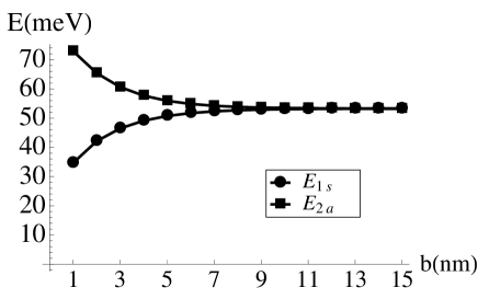
Figure 2: The energies of GaAs/Ga_0.8Al_0.2As DQW as a functions of the central barrier width at $a=6~{}\textrm{nm}$.

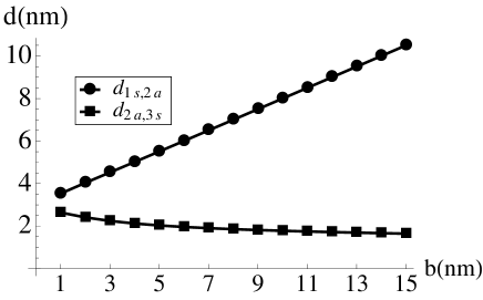
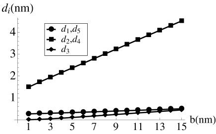
a) b)

Figure 3: a) Dipole matrix elements $d_{1s,2a}$ and $d_{2a,3s}$ as a function of barrier width $b$. b) Contribution of individual regions to dipole matrix $d_{1s,2a}$.

In the first and fifth regions the contribution to dipole is

$$d_{1}=d_{5}=d_{1N}/d_{1D}\,,$$ (2.3db)

where

$$d_{1N} = k_{s}k_{a}\big{[}2+(2a+b)(\chi_{s}+\chi_{a})\big{]}r_{s}r_{a}\,,$$ (2.3dc)

$$r_{s} = \sqrt{\chi_{s}\big{[}(k_{s}^{2}-\chi_{s}^{2})+(k_{s}^{2}+\chi_{s}^{2})\cosh b\chi_{s}\big{]}}\,,$$

$$r_{a} = \sqrt{\chi_{a}\big{[}-(k_{a}^{2}-\chi_{a}^{2})+(k_{a}^{2}+\chi_{a}^{2})\cosh b\chi_{a}\big{]}}\,,$$

and

$$d_{1D} = 2(\chi_{s}+\chi_{a})^{2}\sqrt{(k_{s}^{2}+\chi_{s}^{2})(k_{a}^{2}+\chi_{a}^{2})}\>\delta_{s}\delta_{a}\,,$$ (2.3dd)

$$\delta_{s} = \Big{(}-\chi_{s}^{2}(1+a\chi_{s})+k_{s}^{2}\big{[}1+(a+b)\chi_{s}\big{]}+$$

$$(k_{s}^{2}+\chi_{s}^{2})\big{[}(1+a\chi_{s})\cosh b\chi_{s}+\sinh b\chi_{s}\big{]}\Big{)}^{1/2},$$

$$\delta_{a} = \Big{(}\chi_{a}^{2}(1+a\chi_{a})-k_{a}^{2}\big{[}1+(a+b)\chi_{a}\big{]}+$$

$$(k_{a}^{2}+\chi_{a}^{2})\big{[}(1+a\chi_{a})\cosh b\chi_{a}+\sinh b\chi_{a}\big{]}\Big{)}^{1/2}.$$

In the second region it is

$$d_{2}=d_{2N}/d_{2D}\,,$$ (2.3de)

where

$$d_{2N} = -\frac{1}{2}r_{s}r_{a}\big{[}(k_{s}-k_{a})^{2}(p_{1}-p_{3})-(k_{s}+k_{a})^{2}(p_{2}-p_{4})\big{]}\,,$$ (2.3df)

$$p_{1} = \big{[}b(k_{s}+k_{a})(k_{s}\chi_{a}+k_{a}\chi_{s})+2k_{s}k_{a}-2\chi_{s}\chi_{a}\big{]}\cos a(k_{s}+k_{a})\,,$$

$$p_{2} = \big{[}b(k_{s}-k_{a})(k_{s}\chi_{a}-k_{a}\chi_{s})-2k_{s}k_{a}-2\chi_{s}\chi_{a}\big{]}\cos a(k_{s}-k_{a})\,,$$

$$p_{3} = \big{[}b(k_{s}+k_{a})(k_{s}k_{a}-\chi_{s}\chi_{a})-2k_{s}\chi_{a}-2k_{a}\chi_{s}\big{]}\sin a(k_{s}+k_{a})\,,$$

$$p_{4} = \big{[}b(k_{a}-k_{s})(k_{s}k_{a}+\chi_{s}\chi_{a})+2k_{a}\chi_{s}-2k_{s}\chi_{a}\big{]}\sin a(k_{s}-k_{a})\,,$$

$$d_{2D}=\frac{(k_{s}^{2}-k_{a}^{2})^{2}}{(\chi_{s}+\chi_{a})^{2}}d_{1D}\,.$$ (2.3dg)

One can see that trigonometric functions, which will give oscillations of matrix elements vs. the well width, appear only here.

The third (barrier) region contribution to dipole is

$$d_{3}=d_{3N}/d_{3D}\,,$$ (2.3dh)

where

$$d_{3N} = -4\rme^{\frac{1}{2}b(\chi_{s}+\chi_{a})}k_{s}k_{a}r_{s}r_{a}\big{[}v_{1}\cosh\frac{b\chi_{a}}{2}+v_{2}\sinh\frac{b\chi_{a}}{2}\big{]}\,,$$ (2.3di)

$$v_{1} = -b\chi_{a}(\chi_{s}^{2}-\chi_{a}^{2})\cosh\frac{b\chi_{s}}{2}+4\chi_{s}\chi_{a}\sinh\frac{b\chi_{s}}{2}\,,$$

$$v_{2} = -2(\chi_{a}^{2}+\chi_{2}^{2})\cosh\frac{b\chi_{s}}{2}+4b\chi_{s}(\chi_{s}^{2}-\chi_{a}^{2})\sinh\frac{b\chi_{s}}{2}\,,$$

and

$$d_{3D} = \frac{1}{2}(\chi_{s}-\chi_{a})^{2}s_{s}s_{a}d_{1D}\,,$$ (2.3dj)

$$s_{s} = \sqrt{\frac{(1+\rme^{b\chi_{s}})^{2}k_{s}^{2}+(-1+\rme^{b\chi_{s}})^{2}\chi_{s}^{2}}{k_{s}^{2}+\chi_{s}^{2}}}\,,$$

$$s_{a} = \sqrt{\frac{(-1+\rme^{b\chi_{a}})^{2}k_{a}^{2}+(1+\rme^{b\chi_{a}})^{2}\chi_{a}^{2}}{k_{a}^{2}+\chi_{a}^{2}}}\,.$$

Figure 2 shows the dependencies of the first two energy levels $E_{1s}$ and $E_{2a}$ as a function of the inner barrier width. The following parameter values that are typical to GaAs/Ga_0.8Al_0.2As DQW heterostructures, were used for production of pictures: $a=6~{}\textrm{nm}$, $b=(1-15)~{}\textrm{nm}$, $V_{c}=V_{b}=0.1671~{}\textrm{eV}$, $m_{0}=0.067m_{e}$, $m_{c}=m_{b}=0.0836m_{e}$, where $m_{e}$ is the electron mass in the vacuum. The increase of energy difference between levels with the decrease of $b$ is assigned to tunnel coupling of levels.

Figure 3a demonstrates, respectively, the size of optical dipole matrix elements between a pairs of adjacent levels, $d_{1s,2a}$ and $d_{2a,3s}$, as a function of barrier width. Figure 3b shows the contribution of individual regions to the dipole $d_{1s,2a}$. It is clear that a general trend and magnitude of dipole elements in figure 3a can be understood if one assumes that only quantum wells contribute to the total dipole. In this approximation the functions $\psi_{1}=\psi_{3}=\psi_{5}=0$ while the $\psi_{2}$ and $\psi_{4}$ can be approximated by half-period sine functions. Then $d_{1s,2a}$ reduces to

$$d_{1s,2a}\approx\frac{2}{a}\int_{0}^{a}\sin\frac{\pi x}{a}\Bigl{(}x-a-\frac{b}{2}\Bigr{)}\bigl{(}-\sin\frac{\pi x}{a}\bigr{)}\mathrm{d}x=\frac{a+b}{2}.$$ (2.3dk)

The formula shows that dipole size increases linearly with the barrier width $b$ as long as $b$ remains much smaller than exciting light period. For $2a-3s$ optical transitions one of sines should be replaced by $\sin(2\pi x/a)$. Then, similar calculation yields $d_{2a,3s}\approx 16a/9\pi^{2}$, which is independent of barrier width. The deviations from the obtained expressions in figure 3a come from the evanescent mode contribution in barrier and confining potential regions.

In conclusion, the presented example shows that application of Gröbner basis algorithm in some cases allows to find closed form expressions for the total wave function and, therefore, to calculate the dipole matrix elements exactly without directly solving the transcendental equations that determines the spectrum of the DQW. Of course, the described method can be applied to other quantum systems for which eigenvalue equations cannot be explicitly solved as well.

References

References

[1]
Goldman I I and Krivchenkov V D 1961 Problems in Quantum
Mechanics (New York: Pergamon Press)
[2]
Deutchman P A 1971 Am. J. Phys.39 952–4
[3]
Deutchman P A and Koelsch D C 1974 Am. J. Phys.42
743–53
[4]
Johnson E A and Williams H T 1982 Am. J. Phys., 50
239–43
[5]
de Menezes O L T and Helman J S 1985 Am. J. Phys.53 1100–2
[6]
Peacock-López E 2006 The Chemical Educator, 11
383–93
[7]
Weisbuch C 1987 Semiconductors and Semimetals ed R Dingle,
(New York: Academic Press), 24 1-134
[8]
Harrison P 2005 Quantum Wells, Wires and Dots ( England:
John Wiley and Sons)
[9]
Manasreh O 2005 Semiconductor Heterojunctions and
Nanostructures (New York: McGraw-Hill)
[10]
Hasbun J E 2002 J. Phys.: Cond.Matter, 14 R143–R175
[11]
Debray P, Gurevich V, Klesse R and Newrock R S 2002 Sem.
Sci. Techn.17 R21–R34
[12]
Bastard G, Ziemelis U O, Delalande C, Voos M, Gossard A C and
Wiegmann W 1984 Solid State Commun., 49 671–4
[13]
Cox D, Little J and O’Shea D. 1998 Ideals, Varieties and
Algorithms (New York: Springer-Verlag)
[14]
BenDaniel D J and Duke C B 1966
Phys. Rev., 152 683–92
[15]
Trott M 2004 The Mathematica Guidebook for Symbolics (New
York: Springer-Verlag), Chap. 1
[16] The details of calculation can be downloaded
in a form of Mathematica notebook from
http//mokslasplius.lt/files/DQW.nb
b)
b)