Probabilistic Voronoi Diagrams for Probabilistic Moving Nearest Neighbor Queries

Abstract

A large spectrum of applications such as location based services and environmental monitoring demand efficient query processing on uncertain databases. In this paper, we propose the probabilistic Voronoi diagram (PVD) for processing moving nearest neighbor queries on uncertain data, namely the probabilistic moving nearest neighbor (PMNN) queries. A PMNN query finds the most probable nearest neighbor of a moving query point continuously. To process PMNN queries efficiently, we provide two techniques: a pre-computation approach and an incremental approach. In the pre-computation approach, we develop an algorithm to efficiently evaluate PMNN queries based on the pre-computed PVD for the entire data set. In the incremental approach, we propose an incremental probabilistic safe region based technique that does not require to pre-compute the whole PVD to answer the PMNN query. In this incremental approach, we exploit the knowledge for a known region to compute the lower bound of the probability of an object being the nearest neighbor. Experimental results show that our approaches significantly outperform a sampling based approach by orders of magnitude in terms of I/O, query processing time, and communication overheads.

1 Introduction

Uncertainty is an inherent property in many database applications that include location based services [1], environmental monitoring [2], and feature extraction systems [3]. The inaccuracy or imprecision of data capturing devices, the privacy concerns of users, and the limitations on bandwidth and battery power introduce uncertainties in different attributes such as the location of an object or the measured value of a sensor. The values of these attributes are stored in a database, known as an uncertain database.

In recent years, query processing on an uncertain database has received significant attention from the research community due to its wide range of applications. Consider a location based application where the location information of users may need to be pre-processed before publishing due to the privacy concern of users. Alternatively, a user may want to provide her position as a larger region in order to prevent her location to be identified to a particular site. In such cases, locations of users are stored as uncertain attributes such as regions instead of points in the database. An application that deals with the location of objects (e.g., post office, hospital) obtained from satellite images is another example of an uncertain database. Since the location information may not be possible to identify accurately from the satellite images due to noisy transmission, locations of objects need to be represented as regions denoting the probable locations of objects. Likewise, in a biological database, objects identified from microscopic images need to be presented as uncertain attributes due to inaccuracies of data capturing devices.

In this paper, we propose a novel concept called Probabilistic Voronoi Diagram (PVD), which has a potential to efficiently process nearest neighbor (NN) queries on an uncertain database. The PVD for a given set of uncertain objects ${o_{1},o_{2},...,o_{n}}$ partitions the data space into a set of Probabilistic Voronoi Cells (PVCs) based on the probability measure. Each cell $PVC(o_{i})$ is a region in the data space, where each data point in this region has a higher probability of being the NN to $o_{i}$ than any other object.

A nearest neighbor (NN) query on an uncertain database, called a Probabilistic Nearest Neighbor (PNN) query, returns a set of objects, where each object has a non-zero probability of being the nearest to a query point. A common variant of the PNN query that finds the most probable NN to a given query point is also called a top-1-PNN query. Existing research focuses on efficient processing of PNN queries [4, 5, 6, 7] and its variants [8, 9, 10] for a static query point. In this paper, we are interested in answering Probabilistic Moving Nearest Neighbor (PMNN) queries on an uncertain database, where data objects are static, the query is moving, and the future path of the moving query is unknown. A PMNN query returns the most probable nearest object for a moving query point continuously.

A straightforward approach for evaluating a PMNN query is to use a sampling-based method, which processes the PMNN query as a sequence of PNN queries at sampled locations on the query path. However, to obtain up-to-date answers, a high sampling rate is required, which makes the sampling-based approach inefficient due to the frequent processing of PNN queries.

To avoid high processing cost of the sampling based approach and to provide continuous results, recent approaches for continuous NN query processing on a point data set rely on safe-region based techniques, e.g., Voronoi diagram [11]. In a Voronoi diagram based approach, the data space is partitioned into disjoint Voronoi cells where all points inside a cell have the same NN. Then, the NN of a query point is reduced to identifying the cell for the query point, and the result of a moving query point remains valid as long as it remains inside that cell. Motivated by the safe-region based paradigm, in this paper we propose a Voronoi diagram based approach for processing a PMNN query on a set of uncertain objects.

Voronoi diagrams for uncertain objects [6, 12] based on a simple distance metric, such as the minimum and maximum distances to objects, result in a large neutral region that contains those points for which no specific NN object is defined. Thus, these are not suitable for processing a PMNN query. In this paper, we propose the PVD that divides the space based on a probability measure rather than using just a simple distance metric.

A naive approach to compute the PVD is to find the top-1-PNN for every possible location in the data space using existing static PNN query processing techniques [4, 5, 8], which is an impractical solution due to high computational overhead. In this paper, we propose a practical solution to compute the PVD for a set of uncertain objects. The key idea of our approach is to efficiently compute the probabilistic bisectors between two neighboring objects that forms the basis of PVCs for the PVD.

After computing the PVD, the most probable NN can be determined by simply identifying the PVC in which the query point is currently located. The result of the query does not change as long as the moving query point remains in the current PVC. A user sends its request as soon as it exits the PVC. Thus, in contrast to the sampling based approach, the PVD ensures the most probable NN for every point of a moving query path is available. Since this approach requires the pre-computation of the whole PVD, we name it the pre-computation approach in this paper.

The pre-computation approach needs to access all the objects from the database to compute the entire PVD. In addition, the PVD needs to be re-computed for any updates (insertion or deletion) to the database. Thus the pre-computation approach may not be suitable for the cases when the query is confined into a small region in the data space or when there are frequent updates in the database. For such cases, we propose an incremental algorithm based on the concept of local PVD. In this approach, a set of surrounding objects and an associated search space, called known region, with respect to the current query position are retrieved from the database. Objects are retrieved based on their probabilistic NN rankings from the current query location. Then, we compute the local PVD based only on the retrieved data set, and develop a probabilistic safe region based PMNN query processing technique. The probabilistic safe region defines a region for an uncertain object where the object is guaranteed to be the most probable nearest neighbor. This probabilistic safe region enables a user to utilize the retrieved data more efficiently and reduces the communication overheads when a client is connected to the server through a wireless link. The process needs to be repeated as soon as the retrieved data set cannot provide the required answer for the moving query point. We name this PMNN query processing technique the incremental approach in this paper.

In summary, we make the following contributions in this paper:

• We formulate the Probabilistic Voronoi Diagram (PVD) for uncertain objects and propose techniques to compute the PVD.

• We provide an algorithm for evaluating PMNN queries based on the pre-computed PVD.

• We propose an incremental algorithm for evaluating PMNN queries based on the concept of local PVD.

• We conduct an extensive experimental study which shows that our PVD based approaches outperform the sampling based approach significantly.

The rest of the paper is organized as follows. Section 2 discusses preliminaries and the problem setup. Section 3 reviews related work. In Section 4, we formulate the concept of PVD and present methods to compute it, focusing on one and two dimensional spaces. In Section 5, we present two techniques: pre-computation approach and incremental approach for processing PMNN queries. Section 6 reports our experimental results and Section 7 concludes the paper.

2 Preliminaries and Problem Setup

Let $O$ be a set of uncertain objects in a $d$-dimensional data space. An uncertain object $o_{i}\in O$, $1\leq i\leq|O|$, is represented by a $d$-dimensional uncertain range $R_{i}$ and a probability density function $(pdf)$ $f_{i}(u)$ that satisfies $\int_{R_{i}}f_{i}(u)du=1$ for $u\in R_{i}$. If $u\notin R_{i}$, then $f_{i}(u)=0$. We assume that the pdf of uncertain objects follow uniform distributions for the sake of easy explication. Our concept of PVD is applicable for other types of distributions. We briefly discuss PVDs for other distributions in Section 4.3). For uniform distribution, the pdf of $o_{i}$ can be expressed as $f_{i}(u)=\frac{1}{Area(R_{i})}$ for $u\in R_{i}$. For example, for a circular object $o_{i}$, the uncertainty region and the pdf are represented as $R_{i}=(c_{i},r_{i})$ and $f_{i}(u)=\frac{1}{\pi r_{i}^{2}}$, respectively, where $c_{i}$ is the center and $r_{i}$ is the radius of the region. We also assume that the uncertainty of objects remain constant.

An NN query on a traditional database consisting of a set of data points (or objects) returns the nearest data point to the query point. An NN query on an uncertain database does not return a single object, instead it returns a set of objects that have non-zero probabilities of being the NN to the query point. Suppose that the database maintains only point locations $c_{1}$, $c_{2}$, and $c_{3}$ for objects $o_{1}$, $o_{2}$, and $o_{3}$, respectively (see Figure 1). Then an NN query with respect to $q$ returns $o_{2}$ as the NN because the distance $dist(c_{2},q)$ is the least among all other objects. In this case, $o_{1}$ and $o_{3}$ are the second and third NNs, respectively, to the query point $q$. If the database maintains the uncertainty regions $R_{1}=(c_{1},r_{1})$, $R_{2}=(c_{2},r_{2})$, and $R_{3}=(c_{3},r_{3})$ for objects $o_{1}$, $o_{2}$, and $o_{3}$, respectively, then the NN query returns all three $(o_{1},p_{1}),(o_{2},p_{2}),(o_{3},p_{3})$ as probable NNs for the query point $q$, where $p_{1}>p_{2}>p_{3}>0$ (see Figure 1).

A Probabilistic Nearest Neighbor (PNN) query [4] is defined as follows:

Definition 2.1

(PNN) Given a set $O$ of uncertain objects in a $d$-dimensional database, and a query point $q$, a PNN query returns a set $P$ of tuples $(o_{i},p_{i})$, where $o_{i}\in O$ and $p_{i}$ is the non-zero probability that the distance of $o_{i}$ to $q$ is the minimum among all objects in $O$.

The probability $p(o_{i},q)$ (or simply $p_{i}$) of an object $o_{i}$ of being the NN to a query point $q$ can be computed as follows. For any point $u\in R_{i}$, where $R_{i}$ is the uncertainty region of an object $o_{i}$, we need to first find out the probability of $o_{i}$ being at $u$ and multiply it by the probabilities of all other objects being farther than $u$ with respect to $q$, and then summing up these products for all $u$ to compute $p_{i}$. Thus, $p_{i}$ can be expressed as follows:

$$p_{i}=\int_{u\in R_{i}}f_{i}(u)\big{(}\prod_{j\neq i}\int_{v\in R_{j}}P(dist(v,q)>dist(u,q))dv\big{)}du,$$ (1)

where the function $P(.)$ returns the probability that a point $v\in R_{j}$ of $o_{j}$ is farther from a point $u\in R_{i}$ of $o_{i}$.

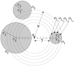
Figure 1: An example of a PNN query

Figure 1 shows a query point $q$, and three objects $o_{1}$, $o_{2}$, and $o_{3}$. Based on Equation 1, the probability $p_{1}$ of object $o_{1}$ being the NN to $q$ can be computed as follows. In this example, we assume a discrete space where the radii of three objects are 5, 2, and 3 units, respectively, and the minimum distance of $o_{1}$ to $q$ is 5 units. Suppose that the dashed circles $(q,5)$, $(q,6)$, $(q,7)$, $(q,8)$, and $(q,9)$ centered at $q$ with radii 5, 6, 7, 8, and 9 units, respectively, divide the uncertain region $R_{1}$ of $o_{1}$ into four sub-regions $o_{1_{1}}$, $o_{1_{2}}$, $o_{1_{3}}$, and $o_{1_{4}}$, where $o_{1_{1}}=(c_{1},r_{1})\cap(q,6)$, $o_{1_{2}}=(c_{1},r_{1})\cap(q,7)-o_{1_{1}}$, $o_{1_{3}}=(c_{1},r_{1})\cap(q,8)-(o_{1_{1}}\cup o_{1_{2}})$, $o_{1_{4}}=(c_{1},r_{1})\cap(q,9)-(o_{1_{1}}\cup o_{1_{2}}\cup o_{1_{3}})$; similarly $R_{2}$ is divided into six sub-regions $o_{2_{1}}$, $o_{2_{2}}$, $o_{2_{3}}$, $o_{2_{4}}$, $o_{2_{5}}$, and $o_{2_{6}}$; $R_{3}$ is divided into three sub-regions $o_{3_{1}}$, $o_{3_{2}}$, and $o_{3_{3}}$.

Then $p_{1}$ can be computed by summing: (i) the probability of $o_{1}$ being within the sub-region $o_{1_{1}}$ multiplied by the probabilities of $o_{2}$ and $o_{3}$ being outside the circular region $(q,6)$, (ii) the probability of $o_{1}$ being within the sub-region $o_{1_{2}}$ multiplied by the probabilities of $o_{2}$ and $o_{3}$ being outside the circular region $(q,7)$, (iii) the probability of $o_{1}$ being within the sub-region $o_{1_{3}}$ multiplied by the probabilities of $o_{2}$ and $o_{3}$ being outside the circular region $(q,8)$, and (iv) the probability of $o_{1}$ being within the sub-region $o_{1_{4}}$ multiplied by the probabilities of $o_{2}$ and $o_{3}$ being outside the circular region $(q,9)$.

As we have discussed in the introduction, in many applications a user may often be interested in the most probable nearest neighbor. In such cases, a PNN only returns the object with the highest probability of being the NN, also known as a top-1-PNN query. In this paper, we address the probabilistic moving NN query that continuously reports the most probable NN for each query point of a moving query.

From Equation 1, we see that finding the most probable NN to a static query point is expensive as it involves costly integration and requires to consider the uncertainty of other objects. Hence, for a moving user that needs to be updated with the most probable answer continuously, it requires repetitive computation of the top object for every sampled location of the moving query. In this paper, we propose PVD based approaches for evaluating a PMNN query.

In this paper, we propose two techniques: a pre-computation approach and an incremental approach to answer PMNN queries. Based on the nature of applications, one can choose any of these techniques that suits best for her purpose. Moreover, both of our techniques fit into any of the two most widely used query processing paradigms: centralized paradigm, and client-server paradigm. In the centralized paradigm the query issuer and the processor reside in the same machine, and the total query processing cost is the main performance measurement metric. On the other hand, in the client-server paradigm, a client issues a query to a server that processes the query, through wireless links such as mobile phone networks. Thus, in the client-server paradigm the performance metric includes both the communication cost and the query processing cost.

In the rest of the paper, we use the following functions: $min(v_{1},v_{2},...,v_{n})$ and $max(v_{1},v_{2},...,v_{n})$ return the minimum and the maximum, respectively, of a given set of values $v_{1}$, $v_{2}$,…,$v_{n}$; $dist(p_{1},p_{2})$ returns the Euclidian distance between two points $p_{1}$ and $p_{2}$; $mindist(p,o)$ and $maxdist(p,o)$ return the minimum and maximum Euclidian distances, respectively, between a point $p$ and an uncertain object $o$.

We also use the following terminologies. When the possible range of values of two uncertain objects overlap then we call them overlapping objects; otherwise they are called non-overlapping objects. If the ranges of two objects are of equal length then we call them equi-range objects; otherwise they are called non-equi-range objects.

3 Background

In this section, we first give an overview of existing PNN query processing techniques on uncertain databases that are closely related to our work. Then we present existing work on Voronoi diagrams.

3.1 Probabilistic Nearest Neighbor

Processing PNN queries on uncertain databases has received significant attention in recent years. In [4], Cheng et al. proposed a numerical integration based technique to evaluate a PNN query for one-dimensional sensor data. In [5], an I/O efficient technique based on numerical integration was developed for evaluating PNN queries on two-dimensional uncertain moving object data. In [7], authors presented a sampling based technique to compute PNN, where both data and query objects are uncertain. Probabilistic threshold NN queries have been introduced in [13], where all objects with probabilities above a specified threshold are reported. In [14], a PNN algorithm was presented where both data and query objects are static trajectories, where the algorithm finds objects that have non-zero probability of any sub-intervals of a given trajectory. Lian et al. [15] presented a technique for a group PNN query that minimizes the aggregate distance to a set of static query points.

The PNN variant, top-$k$-PNN query reports top $k$ objects which have higher probabilities of being the nearest than other objects in the database [8, 9, 10]. Among these works, techniques [9, 10] aim to reduce I/O and CPU costs independently. In [8], the authors proposed a unified cost model that allows interleaving of I/O and CPU costs while processing top-$k$-PNN queries. This method [8] uses lazy computational bounds for probability calculation which is found to be very efficient for finding top-$k$-PNN.

Any existing methods for static PNN queries [4, 5, 7] or its variants [8, 9, 10] can be used for evaluating PMNN queries which process the PMNN query as a sequence of PNN queries at sampled locations on the query path. Since in this paper we are only interested in the most probable answer, we use the recent technique [8] to compute top-1-PNN for processing PMNN queries in a comparative sampling based approach and also for the probability calculation in the PVD.

Some techniques [16, 17] have been proposed for answering PNN queries (including top-$k$-PNN) for existentially uncertain data, where objects are represented as points with associated membership probabilities. However, these techniques are not related to our work as they do not support uncertainty in objects’ attributes. Our problem should also not be confused with maximum likelihood classifiers [18] where they use statistical decision rules to estimate the probability of an object being in a certain class, and assign the object to the class with the highest probability.

All of the above mentioned schemes assume a static query point for PNN queries. Though, continuous processing of NN queries for a moving query point on a point data set was also a topic of interest for many years [19], we are the first to address such queries on an uncertain data set. In this paper, we propose efficient techniques for probabilistic moving NN queries on an uncertain database, where we continuously report the most probable NN for a moving query point.

3.2 Voronoi Diagrams

The Voronoi diagram [11] is a popular approach for answering both static and continuous nearest neighbor queries for two-dimensional point data [20]. Voronoi diagrams for extended objects (e.g., circular objects) [21] have been proposed that use boundaries of objects, i.e., minimum distances to objects, to partition the space. However, these objects are not uncertain, and thus, [21] cannot be used for PNN queries.

Voronoi diagrams for uncertain objects have been proposed that can divide the space for a set of sparsely distributed objects [6, 12]. Both of these approaches are based on the distance metric, where $mindist$ and $maxdist$ to objects are used to calculate the boundary of the Voronoi edges.

The Voronoi diagram of [12] can be described as follows.

Let $R_{1},R_{2},...,R_{n}$ be the regions of a set $O$ of uncertain objects $o_{1},o_{2},...,o_{n}$, respectively. Then a set of sub-regions or cells $V_{1},V_{2},...,V_{n}$ in the data space can be determined such that a point in $V_{i}$ must be closer to any point in $R_{i}$ than to any point in any other object’s region. For two objects $o_{i}$ and $o_{j}$, let $H(i,j)$ be the set of points in the space that are at least as close to any point in $R_{i}$ as any point in $R_{j}$, i.e.,

$$H(i,j)=\{p\|\forall x\in R_{i}\forall y\in R_{j}~{}dist(p,x)\leq dist(p,y)\},$$

where $p$ is a point in the data space.

Then, the cell $V_{i}$ of object $o_{i}$ can be defined as follows:

$$V_{i}=\cap_{j\neq i}H(i,j).$$

The boundary $B(i,j)$ of $H(i,j)$ can be defined as a set of points in $H(i,j)$, where $p\in B(i,j)$ and $maxdist(p,o_{i})=mindist(p,o_{j})$. If the regions are circular, the boundary of object $o_{i}$ with $o_{j}$ is a set of points $p$ that holds the following condition:

$$dist(p,c_{i})+r_{i}=dist(p,c_{j})-r_{j},$$

where $c_{i}$ and $c_{j}$ are the centers and $r_{i}$ and $r_{j}$ are the radii of the regions for objects $o_{i}$ and $o_{j}$, respectively.

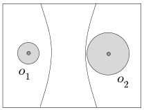
Figure 2: A guaranteed Voronoi diagram

Since $r_{i}$ and $r_{j}$ are constants, the points $p$ that satisfy the above equation lie on the hyperbola (with foci $c_{i}$ and $c_{j}$) arm closest to $o_{i}$. Figure 2 shows an example of this Voronoi diagram for uncertain objects $o_{1}$ and $o_{2}$. The figure also shows the neutral region (the region between two hyperbolic arms) for which the NN cannot be defined by using this Voronoi diagram. Since this Voronoi diagram divides the space based on only the distances (i.e., mindist and maxdist of objects), there may not exist any partition of the space when there is no point such that mindist of an object is equal to maxdist of the other object, i.e., when the regions of objects overlap or too close to each other.

In this approach, a Voronoi cell $V_{i}$ only contains those points in the data space that have $o_{i}$ as the nearest object with probability one. Thus, this diagram is called a guaranteed Voronoi diagram for a given set of uncertain objects. However, in our application domain, an uncertain database can contain objects with overlapping ranges or objects with close proximity (or densely populated) [4, 5, 8]. Hence a PNN query returns a set of objects (possibly more than one) which have the possibilities of being the NN to the query point. Having such a data distribution, the guaranteed Voronoi diagram cannot divide the space at all, and as a result the neutral regions cover most of the data space for which no nearest object can be determined. However, for an efficient PMNN query evaluation we need to continuously find the most probable nearest object for each point of the query path. We propose a Probabilistic Voronoi Diagram (PVD) that works for any distribution of data objects.

Cheng et al. [6] also propose a Voronoi diagram for uncertain data, called Uncertain-Voronoi diagram (UV-diagram). The UV-diagram partitions the space based on the distance metric similar to the guaranteed Voronoi diagram [12]. For each uncertain object $o_{i}$, the UV-diagram defines a region (or UV-cell) where $o_{i}$ has a non-zero probability of being the NN for any point in this region. The main difference of the UV-diagram from the guaranteed Voronoi diagram is that the guaranteed Voronoi diagram concerns about finding the region for a object where the object is guaranteed to be the NN for any point in this region, on the other hand UV-diagram concerns about defining a region for an object where the object has a chance of being the NN for any point in this region. For example, in Figure 2, all points that are left side of the hyperbolic arm closest to $o_{2}$ have non-zero probabilities of $o_{1}$ being the NN, and thus the region left to this hyperbolic line (i.e., closest to $o_{2}$) defines the UV-cell for object $o_{1}$. Similarly, the region right to the hyperbolic line closest to $o_{1}$ defines the UV-cell for object $o_{2}$. Since both UV-diagram and guaranteed Voronoi diagram are based on the concept of similar distance metrics, the UV-diagram suffers from similar limitations as of the guaranteed Voronoi diagram (as discussed above) and is not suitable for our purpose.

4 Probabilistic Voronoi Diagram

A Probabilistic Voronoi Diagram (PVD) is defined as follows:

Definition 4.1

(PVD) Let $O$ be a set of uncertain objects in a $d$-dimensional data space. The probabilistic Voronoi diagram partitions the data space into a set of disjoint regions, called Probabilistic Voronoi Cells (PVCs). The PVC of an object $o_{i}\in O$ is a region or a set of non-contiguous region, denoted by $PVC(o_{i})$, such that $p(o_{i},q)>p(o_{j},q)$ for any point $q\in PVC(o_{i})$ and for any object $o_{j}\in O-\{o_{i}\}$, where $p(o_{i},q)$ and $p(o_{j},q)$ are the probabilities of $o_{i}$ and $o_{j}$ of being the NNs to $q$.

The basic idea of computing a PVD is to identify the PVCs of all objects. To find a PVC of an object, we need to find the boundaries of the PVC with all neighboring objects. The boundary line/curve that separates two neighboring PVCs is called the probabilistic bisector of two corresponding objects, as both objects have equal probabilities of being the NNs for any point on the boundary. Let $o_{i}$ and $o_{j}$ be two uncertain objects, $pb_{o_{i}o_{j}}$ be the probabilistic bisector of $o_{i}$ and $o_{j}$ that separates $PVC(o_{i})$ and $PVC(o_{j})$. Then, for any point $q\in pb_{o_{i}o_{j}}$, $p(o_{i},q)=p(o_{j},q)$, and for any point $q\in PVC(o_{i})$, $p(o_{i},q)>p(o_{j},q)$, and for any point $q\in PVC(o_{j})$, $p(o_{i},q)<p(o_{j},q)$.

A naive approach to compute the PVD requires the processing of PNN queries by using Equation 1 at every possible location in the data space for determining the PVCs based on the calculated probabilities. This approach is prohibitively expensive in terms of computational cost and thus impractical. In this paper, we propose an efficient and practical solution for computing the PVD for uncertain objects. Next, we show how to efficiently compute PVDs, focusing on 1-dimensional (1D) and 2-dimensional (2D) spaces. We briefly discuss higher dimensional cases at the end of this section.

4.1 Probabilistic Voronoi Diagram in a 1D Space

Applications such as environmental monitoring, feature extraction systems capture one dimensional uncertain attributes, and store these values in a database. In this section, we derive the PVD for 1D uncertain objects.

An uncertain 1D object $o_{i}$ can be represented as a range $[l_{i},u_{i}]$, where $l_{i}$ and $u_{i}$ are lower and upper bounds of the range. Let $m_{i}$ and $n_{i}$ be the midpoint and the length of the range $[l_{i},u_{i}]$, i.e., $m_{i}=\frac{l_{i}+u_{i}}{2}$ and $n_{i}=u_{i}-l_{i}$. The probabilistic bisector $pb_{o_{i}o_{j}}$ of two 1D objects $o_{i}$ and $o_{j}$ is a point $x$ within the range $[min(l_{i},l_{j}),max(u_{i},u_{j})]$ such that $p(o_{i},x)=p(o_{j},x)$, and $p(o_{i},x^{\prime})>p(o_{j},x^{\prime})$ for any point $x^{\prime}<x$ and $p(o_{i},x^{\prime\prime})<p(o_{j},x^{\prime\prime})$ for any point $x^{\prime\prime}>x$. Since only the equality condition is not sufficient, other two conditions must also hold. In our proof for lemmas, we will show that a probabilistic bisector needs to satisfy all three conditions.

For example, Figure 3(b) shows two uncertain objects $o_{1}$ and $o_{2}$, and their probabilistic bisector $pb_{o_{1}o_{2}}$ as a point $x$. In this example, the lengths of range for $o_{1}$ and $o_{2}$ are $n_{1}=8$ and $n_{2}=4$, respectively, and the minimum distances from $x$ to $o_{1}$ and $o_{2}$ are $d_{1}=1$ and $d_{2}=3$, respectively. Then based on Equation 1, we can compute the probabilities of $o_{1}$ and $o_{2}$ of being the NN to $x$ as follows:

$$p(o_{1},x) =\frac{2}{8}\cdot\frac{4}{4}+\frac{1}{8}\cdot\frac{3}{4}+\frac{1}{8}\cdot\frac{2}{4}+\frac{1}{8}\cdot\frac{1}{4}=\frac{14}{32},$$

and

$$p(o_{2},x) =\frac{1}{4}\cdot\frac{5}{8}+\frac{1}{4}\cdot\frac{4}{8}+\frac{1}{4}\cdot\frac{3}{8}+\frac{1}{4}\cdot\frac{2}{8}=\frac{14}{32}.$$

A naive approach for finding the $pb_{o_{i}o_{j}}$ requires the computation of probabilities (using Equation 1) of $o_{i}$ and $o_{j}$ for every position within the range $[min(l_{i},l_{j}),max(u_{i},u_{j})]$. To avoid high computational overhead of this naive approach, in our method we show that for two equi-range objects (i.e., $n_{i}=n_{j}$), we can always directly compute the probabilistic bisector (see Lemma 4.1) by using the upper and lower bounds of two candidate objects. Similarly, we also show that for two non-equi-range objects, where $n_{i}\neq n_{j}$, we can directly compute the probabilistic bisector for certain scenarios shown in Lemmas 4.2-4.3, and for the remaining scenarios of non-equi-range objects we exploit these lemmas to find probabilistic bisectors at reduced computational cost.

Figure 3: Scenarios of lemmas

Next, we present the lemmas for 1D objects. Lemma 4.1 gives the probabilistic bisector of two equi-range objects, overlapping and non-overlapping. Figure 3(a) is an example of a non-overlapping case. (Note that if $l_{i}=l_{j}$ and $u_{i}=u_{j}$, then two objects $o_{i}$ and $o_{j}$ are assumed to be the same and no probabilistic bisector exists between them.)

Lemma 4.1

Let $o_{i}$ and $o_{j}$ be two objects where $m_{i}\neq m_{j}$. If $n_{i}=n_{j}$, then the probabilistic bisector $pb_{o_{i}o_{j}}$ of $o_{i}$ and $o_{j}$ is the bisector of $m_{i}$ and $m_{j}$.

Proof 4.1

Let $o_{i}$ and $o_{j}$ be two equi-range objects, i.e., $n_{i}=n_{j}$. Let $x$ be the bisector of two midpoints $m_{i}$ and $m_{j}$, i.e., $x=\frac{m_{i}+m_{j}}{2}$.

Then, by using Equation 1, we can calculate the probability of $o_{i}$ being the NN to $x$ as follows.

$$p(o_{i},x) =\sum_{s=1}^{n_{i}-1}\frac{1}{n_{i}}\frac{n_{j}-s}{n_{j}}.$$

Similarly, we can calculate the probability of $o_{j}$ being the NN to $x$, as follows.

$$p(o_{j},x) =\sum_{s=1}^{n_{j}-1}\frac{1}{n_{j}}\frac{n_{i}-s}{n_{i}}.$$

If we put $n_{i}=n_{j}$ in the above two equations, we have $p(o_{i},x)=p(o_{j},x)$. Thus, the probabilities of $o_{i}$ and $o_{j}$ of being the NN from the point $x$ are equal.

Now, let $x^{\prime}=\frac{m_{i}+m_{j}}{2}-\epsilon$ be a point on the left side of $x$. Then we can calculate the probability of $o_{i}$ of being the NN to $x^{\prime}$

$$p(o_{i},x^{\prime}) =2\epsilon\frac{n_{j}}{n_{i}n_{j}}+\sum_{s=1}^{n_{i}-2\epsilon}\frac{1}{n_{i}}\frac{n_{j}-s}{n_{j}}.$$

Similarly, we can calculate the probability of $o_{j}$ being the NN to $x^{\prime}$, as follows.

$$p(o_{j},x^{\prime}) =\sum_{s=2\epsilon+1}^{n_{i}-1}\frac{1}{n_{j}}\frac{n_{i}-s}{n_{i}}.$$

Now, if we put $n_{i}=n_{j}$ in the above two equations, then we have $p(o_{i},x^{\prime})>p(o_{j},x^{\prime})$ at $x^{\prime}$. Similarly we can prove that $p(o_{i},x^{\prime\prime})<p(o_{j},x^{\prime\prime})$ for a point $x^{\prime\prime}$ on the right side of $x$.

Thus, we can conclude that $x$ is the probabilistic bisector of $o_{i}$ and $o_{j}$, i.e., $pb_{o_{i}o_{j}}=x$.

The following lemma shows how to compute the probabilistic bisector of two non-equi-range objects that are non-overlapping (see Figure 3(b)).

Lemma 4.2

Let $o_{i}$ and $o_{j}$ be two non-overlapping objects, where $n_{i}\neq n_{j}$. If there are no other objects within the range $[min(l_{i},l_{j}),max(u_{i},u_{j})]$, then the probabilistic bisector $pb_{o_{i}o_{j}}$ of $o_{i}$ and $o_{j}$ is the bisector of $m_{i}$ and $m_{j}$.

Proof 4.2

Let $n_{i}>n_{j}$, and $x$ be the bisector of two midpoints $m_{i}$ and $m_{j}$ of objects $o_{i}$ and $o_{j}$, respectively, i.e., $x=\frac{m_{i}+m_{j}}{2}$, and the minimum distances from $x$ to $o_{i}$ and $o_{j}$ are $d_{i}$ and $d_{j}$, respectively.

Then, by using Equation 1, we can calculate the probability of $o_{i}$ being the NN to $x$ as follows.

$$p(o_{i},x) =(d_{j}-d_{i})\frac{1}{n_{i}}\frac{n_{j}}{n_{j}}+\sum_{s=1}^{n_{j}-1}\frac{1}{n_{i}}\frac{n_{j}-s}{n_{j}}$$

$$=(d_{j}-d_{i})\frac{n_{j}}{n_{i}n_{j}}+\frac{n_{j}(n_{j}-1)}{2n_{i}n_{j}}.$$

Similarly, we can calculate the probability of $o_{j}$ being the NN to $x$ as follows.

$$p(o_{j},x) =\sum_{s=1}^{n_{j}}\frac{1}{n_{j}}\frac{n_{i}-(d_{j}-d_{i}+s)}{n_{i}}.$$

Since, we have $d_{j}-d_{i}=\frac{n_{i}-n_{j}}{2}$, i.e., $n_{i}=2(d_{j}-d_{i})+n_{j}$. By replacing $n_{i}$ in the numerator of $p(o_{j},x)$, we can have the following,

$$p(o_{j},x) =\sum_{s=1}^{n_{j}}\frac{1}{n_{j}}\frac{2(d_{j}-d_{i})+n_{j}-(d_{j}-d_{i}+s)}{n_{i}}$$

$$=(d_{j}-d_{i})\frac{n_{j}}{n_{i}n_{j}}+\frac{n_{j}(n_{j}-1)}{2n_{i}n_{j}}.$$

Since $p(o_{i},x)=p(o_{j},x)$, we have $pb_{o_{i}o_{j}}=x$.

On the other hand, let $x^{\prime}=\frac{m_{i}+m_{j}}{2}-\epsilon$ be a point on the left side of the probabilistic bisector.

Then, by using Equation 1, we can calculate the probability of $o_{i}$ being the NN to $x^{\prime}$ as follows.

$$p(o_{i},x^{\prime}) =(d_{j}-d_{i}+2\epsilon)\frac{n_{j}}{n_{i}n_{j}}+\frac{n_{j}(n_{j}-1)}{2n_{i}n_{j}}.$$

Similarly, we can calculate the probability of $o_{j}$ being the NN to $x^{\prime}$, as follows.

$$p(o_{j},x^{\prime}) =(d_{j}-d_{i}-2\epsilon)\frac{n_{j}}{n_{i}n_{j}}+\frac{n_{j}(n_{j}-1)}{2n_{i}n_{j}}.$$

So, we can say $p(o_{i},x^{\prime})>p(o_{j},x^{\prime})$ for a point $x^{\prime}$ on the left side of $pb_{o_{i}o_{j}}$. Similarly we can prove that $p(o_{i},x^{\prime\prime})<p(o_{j},x^{\prime\prime})$ for a point $x^{\prime\prime}$ on the right side of $pb_{o_{i}o_{j}}$.

For two non-equi-range objects that are overlapping, the following lemma directly computes the probabilistic bisector for the scenarios where lower, upper, or mid-point values of two candidate objects are same (see Figure 3(c), (d), and (e)).

Lemma 4.3

Let $o_{i}$ and $o_{j}$ be two overlapping objects, where $n_{i}\neq n_{j}$, $l_{i}\leq l_{j}\leq u_{j}\leq u_{i}$, and there are no other objects within the range $[min(l_{i},l_{j}),max(u_{i},u_{j})]$.

1. If $l_{i}=l_{j}$, then the probabilistic bisector $pb_{o_{i}o_{j}}$ of $o_{i}$ and $o_{j}$ is the bisector of $m_{i}$ and $u_{j}$.

2. If $u_{i}=u_{j}$, then the probabilistic bisector $pb_{o_{i}o_{j}}$ of $o_{i}$ and $o_{j}$ is the bisector of $m_{i}$ and $l_{j}$.

3. If $m_{i}=m_{j}$, then the probabilistic bisectors $pb_{o_{i}o_{j}}$ of $o_{i}$ and $o_{j}$ are the bisectors of $l_{i}$ and $l_{j}$, and $u_{i}$ and $u_{j}$.

Proof 4.3

Let $n_{i}>n_{j}$, $l_{i}=l_{j}$, $x=\frac{m_{i}+l_{j}}{2}$, and $d$ be the distance from $x$ to both $m_{i}$ and $l_{j}$.

Then, by using Equation 1, we can calculate the probability of $o_{i}$ being the NN to $x$ as follows.

$$p(o_{i},x) =\sum_{s=1}^{d}\frac{2}{n_{i}}\frac{n_{j}}{n_{j}}+\sum_{s=1}^{n_{j}-1}\frac{2}{n_{i}}\frac{n_{j}-s}{n_{j}}$$

$$=\frac{2d}{n_{i}}+\frac{n_{j}(n_{j}-1)}{n_{i}n_{j}}.$$

Similarly, we can calculate the probability of $o_{j}$ being the NN to $x$ as follows.

$$p(o_{j},x) =\sum_{s=1}^{n_{j}}\frac{1}{n_{j}}\frac{n_{i}-(2d+2s)}{n_{i}}.$$

However, $\frac{n_{i}}{2}-n_{j}=2d$, that is $n_{i}=4d+2n_{j}$. By replacing $n_{i}$ in the numerator and simplifying the term, we can have the following, $p(o_{j},x)=\frac{2d}{n_{i}}+\frac{n_{j}(n_{j}-1)}{n_{i}n_{j}}$. Since $p(o_{i},x)=p(o_{j},x)$, $pb_{o_{i}o_{j}}=x$. Similar to Lemma 4.2, we can prove that $p(o_{i},x^{\prime})>p(o_{j},x^{\prime})$ for any point $x^{\prime}$ on the left, and $p(o_{i},x^{\prime\prime})<p(o_{j},x^{\prime\prime})$ for any point $x^{\prime\prime}$ on the right side of $pb_{o_{i}o_{j}}$.

Similarly, we can prove the case for $u_{i}=u_{j}$.

Let $m_{i}=m_{j}$, $x_{1}=\frac{l_{i}+l_{j}}{2}$, and $d$ be the distance from $x_{1}$ to both $l_{i}$ and $l_{j}$.

Then, by using Equation 1, we can calculate the probability of $o_{i}$ being the NN to $x_{1}$ as follows.

$$p(o_{i},x_{1}) =\sum_{s=1}^{d}\frac{2}{n_{i}}\frac{n_{j}}{n_{j}}+\sum_{s=1}^{n_{j}-1}\frac{1}{n_{i}}\frac{n_{j}-s}{n_{j}}$$

$$=\frac{2d}{n_{i}}+\frac{n_{j}(n_{j}-1)}{2n_{i}n_{j}}.$$

Similarly, we can calculate the probability of $o_{j}$ being the NN to $x_{1}$ as follows.

$$p(o_{j},x_{1})=\sum_{s=1}^{n_{j}}\frac{1}{n_{j}}\frac{n_{i}-(2d+s)}{n_{i}}.$$

However, $\frac{n_{i}}{2}-\frac{n_{j}}{2}=2d$, that is $n_{i}=4d+n_{j}$. By replacing $n_{i}$ in the numerator and simplifying the term, we can have the following, $p(o_{j},x_{1})=\frac{2d}{n_{i}}+\frac{n_{j}(n_{j}-1)}{2n_{i}n_{j}}$. Since $p(o_{i},x^{\prime})=p(o_{j},x^{\prime})$, we have $pb_{o_{i}o_{j}}=x_{1}$. Similar to Lemma 4.2, we can prove that $p(o_{i},x^{\prime})>p(o_{j},x^{\prime})$ for any point $x^{\prime}$ on the left, and $p(o_{i},x^{\prime\prime})<p(o_{j},x^{\prime\prime})$ for any point $x^{\prime\prime}$ on the right side of $pb_{o_{i}o_{j}}$.

Similarly, we can prove that the other probabilistic bisector exists at $x_{2}=\frac{u_{i}+u_{j}}{2}$, as the case is symmetric to that of $x_{1}$.

Note that, since $n_{i}>n_{j}$ and $m_{i}=m_{j}$, $o_{i}$ completely contains $o_{j}$. Thus the probability of $o_{j}$ is higher than that of $o_{i}$ around the mid-point ($m_{i}$), and the probability of $o_{i}$ is higher than that of $o_{j}$ towards the boundary points ($l_{i}$ and $u_{i}$). Therefore in this case, we have two probabilistic bisectors between $o_{i}$ and $o_{j}$.

Figures 3(c-e) show an example of three cases as described in Lemma 4.3. Figure 3(c) shows the first case for objects $o_{1}$ and $o_{2}$, where $l_{1}=l_{2}$ and $pb_{o_{1}o_{2}}=\frac{m_{1}+u_{2}}{2}$. Similarly, Figure 3(d) shows an example of the second case for objects $o_{1}$ and $o_{2}$, where $u_{1}=u_{2}$ and $pb_{o_{1}o_{2}}=\frac{m_{1}+l_{2}}{2}$. Finally, Figure 3(e) shows an example of the third case for objects $o_{1}$ and $o_{2}$, where $m_{1}=m_{2}$, and $x_{1}=\frac{l_{1}+l_{2}}{2}$ and $x_{2}=\frac{u_{1}+u_{2}}{2}$ are two probabilistic bisectors. In such a case, two probabilistic bisectors, $x_{1}$ and $x_{2}$, divide the space into three subspaces. That means, the Voronoi cell of object $o_{1}$ comprises of two disjoint subspaces. In Figure 3(e), the subspace left to $x_{1}$ and the subspace right to $x_{2}$ form the Voronoi cell of $o_{1}$, and the subspace bounded by $x_{1}$ and $x_{2}$ forms the Voronoi cell of $o_{2}$.

Apart from the above mentioned scenarios, the remaining scenarios of two overlapping non-equi-range objects are shown in Figure 4, where it is not possible to compute the probabilistic bisector directly by using lower and upper bounds of two candidate objects. In these scenarios, Lemma 4.3 can be used for choosing a point, called the initial probabilistic bisector, which approximates the actual probabilistic bisector and thereby reducing the computational overhead. Figure 4 (a), (b), (c) show three scenarios, where three cases of Lemma 4.3 (1), (2), (3), are used to compute the initial probabilistic bisector, respectively, for our algorithm. We will see (in Algorithm 1) how to use our lemmas to find the probabilistic bisectors for these scenarios.

Figure 4: Remaining scenarios

So far we have assumed that no other objects exist within the ranges of two candidate objects. However, the probabilities of two candidate objects may change in the presence of any other objects within their ranges (as shown in Equation 1). Only the probabilistic bisector of two equi-range objects remains the same in the presence of any other object within their ranges.

Let $o_{k}$ be the third object that overlaps with the range $[min(l_{i},l_{j}),max(u_{i},u_{j})]$ for the case in Figure 3(a). Then, using Equation 1, we can calculate the NN probability of object $o_{i}$ from $x$ as follows.

$$p(o_{i},x) =\sum_{s=1}^{n_{i}-1}\frac{1}{n_{i}}\frac{n_{j}-s}{n_{j}}\frac{n_{k}-s}{n_{k}}.$$

Similarly, we can calculate the NN probability of object $o_{j}$ from $x$ as follows.

$$p(o_{j},x) =\sum_{s=1}^{n_{j}-1}\frac{1}{n_{j}}\frac{n_{i}-s}{n_{i}}\frac{n_{k}-s}{n_{k}}.$$

Since $n_{i}=n_{j}$, we have $p(o_{i},x)=p(o_{j},x)$ and $pb_{o_{i}o_{j}}=x$. Therefore, the probabilistic bisector $pb_{o_{i}o_{j}}$ does not change with the presence a third object.

Therefore, for scenarios, except for the case when two candidate objects are equi-range, when any other object exists within the ranges two candidate objects, we again use one of the Lemmas 4.1-4.3 to compute the initial probabilistic bisector, and then find the actual probabilistic bisector. For example, if two non-equi-range candidate objects do not overlap each other (see Figure 3(b)) and a third object exists, which is not shown in figure, within the range of these two candidate objects, then we use Lemma 4.2 to find the initial probabilistic bisector. Similarly, we choose the corresponding lemmas for other scenarios to compute initial probabilistic bisectors. Then we use these computed initial probabilistic bisectors to find actual probabilistic bisectors.

The position of a probabilistic bisector depends on the relative positions and the uncertainty regions of two candidate objects. We have shown that for some scenarios the probabilistic bisectors can be directly computed using the proposed lemmas. In some other scenarios, there is no straightforward way to compute probabilistic bisectors. For this latter case, the initial probabilistic bisector of two candidate objects is chosen based on the actual probabilistic bisector of the scenario that can be directly computed and has the most similarity (relative positions of candidate objects) with two candidate objects. This ensures that the initial probabilistic bisector is essentially close to the actual probabilistic bisector.

$pb_{o_{i}o_{j}}\leftarrow\emptyset$AlgoLine0.0.1

AlgoLine0.0.2

if $o_{i}$ and $o_{j}$ satisfy one of the Lemmas 4.1- 4.3 then  $pb_{o_{i}o_{j}}\leftarrow BisectorBasedOnLemmas(o_{i},o_{j},O)$ AlgoLine0.0.3

else  (any pair of objects that does not satisfy Lemmas 4.1- 4.3) AlgoLine0.0.4

if $o_{i}$ and $o_{j}$ do not overlap then  $ipb\leftarrow Bisector(m_{i},m_{j})$ AlgoLine0.0.5

$pb_{o_{i}o_{j}}\leftarrow FindProbBisector1D(o_{i},o_{j},ipb,O)$AlgoLine0.0.6

else  (three possible cases for overlapping pairs of objects (Figure 4)) AlgoLine0.0.7

(assume $l_{i}\leq l_{j}$ (the other case $l_{i}\geq l_{j}$ is symmetric))AlgoLine0.0.8

if $l_{i}<l_{j}$ and $u_{j}<u_{i}$ then  $ipb_{1}\leftarrow Bisector(l_{i},l_{j})$ AlgoLine0.0.9

$ipb_{2}\leftarrow Bisector(u_{i},u_{j})$AlgoLine0.0.10

AlgoLine0.0.11

$pb_{o_{i}o_{j}}\leftarrow FindProbBisector1D(o_{i},o_{j},ipb_{1},O)\cup FindProbBisector1D(o_{i},o_{j},ipb_{2},O)$AlgoLine0.0.12

else if $l_{j}-l_{i}<u_{j}-u_{i}$ then  $ipb\leftarrow Bisector(m_{j},u_{i})$ AlgoLine0.0.13

$pb_{o_{i}o_{j}}\leftarrow FindProbBisector1D(o_{i},o_{j},ipb,O)$AlgoLine0.0.14

  else  $ipb\leftarrow Bisector(m_{i},l_{j})$ AlgoLine0.0.15

$pb_{o_{i}o_{j}}\leftarrow FindProbBisector1D(o_{i},o_{j},ipb,O)$AlgoLine0.0.16

      return $pb_{o_{i}o_{j}}$;

Algorithm 1 ProbBisector1D($o_{i},o_{j},O$)

0.16

0.16

0.16

0.16

0.16

0.16

0.16

0.16

0.16

0.16

0.16

0.16

0.16

0.16

0.16

0.16

Algorithms:

Based on the above lemmas, Algorithm 1 summarizes the steps of computing the probabilistic bisector $pb_{o_{i}o_{j}}$ for any two objects $o_{i}$ and $o_{j}$, where $O$ is a given set of objects and $o_{i},o_{j}\in O$. If $o_{i}$ and $o_{j}$ satisfy any of Lemmas 4.1-4.3 the algorithm directly computes $pb_{o_{i}o_{j}}$ (Lines 1.2- 1.3). Otherwise, if any other object exists within the range of two candidate non-equi-range objects $o_{i}$ and $o_{j}$, or two candidate non-equi-range objects fall in any of the scenarios shown in Figure 4. The algorithm first computes an initial probabilistic bisector $ipb$ using our lemmas, where the given scenario has the most similarity in terms of relative positions of candidate objects to the corresponding lemma. Then, the algorithm uses the function $FindProbBisector1D$ to find $pb_{o_{i}o_{j}}$ by using $ipb$ as a base.

After computing the $ipb$ the algorithm calls a function $FindProbBisector1D$ to find the probabilistic bisector $pb_{o_{i}o_{j}}$ (Lines 1.8, 1.15, 1.18, and 1.21).

The function $FindProbBisector1D$ computes $pb_{o_{i}o_{j}}$ by refining $ipb$. If the probabilities of $o_{i}$ and $o_{j}$ of being the NN from $ipb$ are equal, then the algorithm returns $ipb$ as the probabilistic bisector. Otherwise, the algorithm decides in which direction from $ipb$ it should continue the search for $pb_{o_{i}o_{j}}$. Let $x=ipb$. We also assume that $o_{i}$ is left to $o_{j}$. If $p(o_{i},x)$ is smaller than $p(o_{j},x)$, then $pb_{o_{i}o_{j}}$ is to the left of $x$ and within the range $[min(l_{i},l_{j}),x]$, otherwise $pb_{o_{i}o_{j}}$ is to the right of $x$ and within the range $[x,max(l_{i},l_{j})]$. Since using lemmas, we choose $ipb$ as close as possible to $pb_{o_{i}o_{j}}$, in most of the cases the probabilistic bisector is found very close to the position of $ipb$. Thus, as an alternative to directly running a binary search within the range, one can perform a step-wise search first, by increasing (or decreasing) the value of $x$ until the probability ranking of two objects swaps. Since the precision of probability measures affects the performance of the above search, we assume that the two probability measures are equal when the difference between them is smaller than a threshold. The value of the threshold can be found experimentally given an application domain.

$PVD\leftarrow\emptyset$AlgoLine0.0.1

$PBL\leftarrow\emptyset$AlgoLine0.0.2

$SortObjects(O)$AlgoLine0.0.3

for each $o_{i}\in O$ do  $o_{j}\leftarrow getNext(O)$ $pb_{o_{i}o_{j}}\leftarrow ProbBisector1D(o_{i},o_{j},O)$ $PBL\leftarrow PBL\cup pb_{o_{i}o_{j}}$ AlgoLine0.0.4

$N\leftarrow getCandidateObjects(O,pb_{o_{i}o_{j}})$AlgoLine0.0.5

for each $o_{k}\in N$ do  $pb_{o_{i}o_{k}}\leftarrow ProbBisector1D(o_{i},o_{k},O)$ $PBL\leftarrow PBL\cup pb_{o_{i}o_{k}}$ AlgoLine0.0.6

AlgoLine0.0.7

  AlgoLine0.0.8

  $SPBL\leftarrow\ SortProbBisectors(PBL)$AlgoLine0.0.9

AlgoLine0.0.10

$o^{\prime}\leftarrow initialMostProbableObject()$AlgoLine0.0.11

AlgoLine0.0.12

while $SPBL$ is not empty do  $pb_{o_{i}o_{j}}\leftarrow popNextPB(SPBL)$ AlgoLine0.0.13

$left\leftarrow LeftSideObject()$AlgoLine0.0.14

$right\leftarrow RightSideObject()$AlgoLine0.0.15

if $PVD$ is empty OR $o^{\prime}=left$ then  $PVD\leftarrow PVD\cup ProbBisector(pb_{o_{i}o_{j}},o_{i},o_{j})$ AlgoLine0.0.16

$o^{\prime}\leftarrow right$ AlgoLine0.0.17

AlgoLine0.0.18

else  $Discard(pb_{o_{i}o_{j}})$ AlgoLine0.0.19

    AlgoLine0.0.20

return $PVD$;

Algorithm 2 ProbVoronoi1D($O$)

0.20

0.20

0.20

0.20

0.20

0.20

0.20

0.20

0.20

0.20

0.20

0.20

0.20

0.20

0.20

0.20

0.20

0.20

0.20

0.20

Finally, Algorithm 2 shows the steps for computing a PVD for a set of 1D uncertain objects $O$. In 1D data space, the PVD contains a list of bisectors that divides the total data space into a set of Voronoi cells or 1D ranges. The basic idea of Algorithm 2 is that, once we have the probabilistic bisectors of all pairs of objects in a sorted list, a sequential scan of the list can find the candidate probabilistic bisectors that comprise the probabilistic Voronoi diagram in 1D space.

To avoid computing probabilistic bisectors for all pairs of objects $o_{i},o_{j}\in O$, we use the following heuristic:

Heuristic 4.1

Let $o_{i}$ be an object in the ordered (in ascending order of $l_{i}$) list of objects $O$, and $o_{j}$ be the next object right to $o_{i}$ in $O$. Let $x=pb_{o_{i}o_{j}}$, and $d=dist(x,l_{i})$. Let $o_{k}$ be an object in $O$. If $dist(x,l_{k})>d$, then the probabilistic bisector $pb_{o_{i}o_{k}}$ of $o_{i}$ and $o_{k}$ is $x^{\prime}$, and $x^{\prime}$ is to the right of $x$, i.e., $x^{\prime}>x$; therefore $pb_{o_{i}o_{k}}$ does not need to be computed.

Algorithm 2 runs as follows. First, the algorithm sorts all objects in ascending order of their lower bounds (Line 2.3). Second, for each object $o_{i}$, it computes probabilistic bisectors of $o_{i}$ with the next object $o_{j}\in O$ and with a set $N$ of objects returned by the function $getCandidateObjects$ based on Heuristic 4.1 (Lines 2.4-2.8). $PBL$ maintains the list all computed probabilistic bisectors. Third, the algorithm sorts the list $PBL$ in ascending order of the position of probabilistic bisectors and assigns the sorted list to $SPBL$ (Line 2.9). Finally, from $SPBL$, the algorithm selects probabilistic bisectors that contribute to the PVD (Lines 2.10-2.19). For this final step, the algorithm first finds the most probable NN $o^{\prime}$ with respect to the starting position of the data space. Then for each $pb_{o_{i}o_{j}}\in SPBL$, the algorithm decides whether $pb_{o_{i}o_{j}}$ is a candidate for the $PVD$ (Lines 2.11-2.19). We assume that $o_{i}$ is the left side object and $o_{j}$ is the right side object of the probabilistic bisector. If $o^{\prime}=o_{i}$, then $pb_{o_{i}o_{j}}$ is included in the $PVD$, and $o^{\prime}$ is updated with the most probable object on the right region of $pb_{o_{i}o_{j}}$ (Line 2.17). Otherwise, $pb_{o_{i}o_{j}}$ is discarded (Line 2.19). This process continues until $SPBL$ becomes empty, and the algorithm finally returns $PVD$.

The proof of correctness and the complexity of this algorithm are provided as follows.

Correctness: Let $SPBL$ be the list of probabilistic bisectors in ascending order of their positions. Let $o^{\prime}$ be the most probable NN with respect to the starting point $l$ of the 1D data space. Let $pb_{o_{i}o_{j}}$ be the next probabilistic bisector fetched from $SPBL$. Now we can have the following two cases: (i) Case 1: $o^{\prime}=o_{i}$. The probability $p_{i}$ of $o_{i}$ being the nearest is the highest for all points starting from $l$ to $pb_{o_{i}o_{j}}$ and the probability $p_{j}$ of $o_{j}$ being the nearest is the highest for points on the right side of $pb_{o_{i}o_{j}}$ until the next valid probabilistic bisector is found. Hence, $pb_{o_{i}o_{j}}$ is a valid probabilistic bisector and is added to the PVD. Then the algorithm updates $o^{\prime}$ by $o_{j}$ since $o_{j}$ will be the most probable on the right of $pb_{o_{i}o_{j}}$ and will be on the left region of the next valid probabilistic bisector. (ii) Case 2: $o^{\prime}\neq o_{i}$. Let us assume that $p_{i}>p^{\prime}$ at $pb_{o_{i}o_{j}}$. We already know that $p^{\prime}>p_{i}$ at the starting point $l$. So there should be some point within the range [$l,pb_{o_{i}o_{j}}$] where $p^{\prime}=p_{i}$, which is the position of the probabilistic bisector of $o^{\prime}$ and $o_{i}$. Since no such bisector is found within this range, $p_{i}>p^{\prime}$ is not true at $pb_{o_{i}o_{j}}$. Thus, $p^{\prime}$ is the highest even at $pb_{o_{i}o_{j}}$, and will remain the highest until it fetches another $pb_{o_{i^{\prime}}o_{j^{\prime}}}$ from $SPBL$, where $o^{\prime}=o_{i^{\prime}}$. The above process continues until the algorithm reaches the end of the data space.

Complexity: The complexity of Algorithm 2 can be determined as follows. Let $C_{b}$ be the cost of computing the probability of an object being the NN of a query point, and $C_{pb}$ be the cost of finding the probabilistic bisector of two objects. The complexity of Algorithm 2 is dominated by the complexity of executing the Lines 2.4-2.8, which is $O(nNC_{pb})$, where $n$ is the total number of objects, and $N$ is the expected number of probabilistic bisectors that need to be computed for each object in $O$. For real data sets, $N$ is found to be a small value since each object has a small number of surrounding objects (in the worst case it can be $n-1$). The cost of $C_{pb}=O(C_{b}\log_{2}D)$, where $D$ is the expected distance between our initial probabilistic bisector $ipb$ and the actual probabilistic bisector. This is because, the cost of finding a probabilistic bisector is $O(1)$ for the cases when our algorithm can directly compute the probabilistic bisector, and for other cases our algorithm first finds $ipb$ by $O(1)$ and then searches for the actual probabilistic bisector using $FindProbBisector1D$ by $O(\log D)$.

4.2 Probabilistic Voronoi Diagram in a 2D Space

In location-based applications, locations of objects such as a passenger and a building, in a 2D space can be uncertain due to the imprecision of data capturing devices or the privacy concerns of users. In these applications, the location of an object $o_{i}$ can be represented as a circular region $R_{i}=(c_{i},r_{i})$, where $c_{i}$ is the center and $r_{i}$ is the radius of the region, and the actual location of $o_{i}$ can be anywhere in $R_{i}$. The area of $o_{i}$ is expressed as $A_{i}=\pi r_{i}^{2}$. In this section, we derive the PVD for 2D uncertain objects.

Similar to the 1D case, a naive approach to find the probabilistic bisector $pb_{o_{i}o_{j}}$ of $o_{i}$ and $o_{j}$ requires an exhaustive computation of probabilities using Equation 1 for every position in a large area. In our approach, we first show that we can directly compute $pb_{o_{i}o_{j}}$ as the bisector $bs_{c_{i}c_{j}}$ of $c_{i}$ and $c_{j}$ when two candidate objects are equi-range (i.e., $r_{i}=r_{j}$). Next, we show that for two non-equi-range objects (i.e., $r_{i}\neq r_{j}$), depending on radii and relative positions of objects $pb_{o_{i}o_{j}}$ slightly shifts from $bs_{c_{i}c_{j}}$. In this case, we use $bs_{c_{i}c_{j}}$ to choose a line, called the initial probabilistic bisector, to approximate the actual probabilistic bisector $pb_{o_{i}o_{j}}$. Although for simplicity of presentation, we will use examples where two candidate objects are non-overlapping, Lemmas 4.4-4.7 also hold for overlapping objects.

For two equi-range uncertain circular objects $o_{i}$ and $o_{j}$, we have the following lemma:

Lemma 4.4

Let $o_{i}$ and $o_{j}$ be two circular uncertain objects with uncertain regions $(c_{i},r_{i})$ and $(c_{j},r_{j})$, respectively. If $r_{i}=r_{j}$, then the probabilistic bisector $pb_{o_{i}o_{j}}$ of $o_{i}$ and $o_{j}$ is the bisector $bs_{c_{i}c_{j}}$ of $c_{i}$ and $c_{j}$.

Proof 4.4

Let $x$ be any point on $bs_{c_{i}c_{j}}$, and $d=mindist(x,o_{i})$(or $mindist(x,o_{j})$). Let there be no other objects within the circular range centered at $x$ with radius $d+2r_{i}$. Suppose circles centered at $x$ with radii $d+1$ to $d+2r_{i}$ partition $o_{i}$ into $2r_{i}$ sub-regions $o_{i_{1}},o_{i_{2}},...,o_{i_{2r_{i}}}$, such that $\sum_{s=1}^{2r_{i}}\frac{o_{i_{s}}}{A_{i}}=1$. Similarly, $o_{j}$ is divided into $2r_{i}$ sub-regions $o_{j_{1}},o_{j_{2}},...,o_{j_{2r_{i}}}$, where $\sum_{s=1}^{2r_{i}}\frac{o_{j_{s}}}{A_{j}}=1$. By using Equation 1, we can calculate the probability of $o_{i}$ being the nearest from $x$, as follows.

$$p(o_{i},x) =\sum_{s=d+1}^{2r_{i}+d}\frac{o_{i_{s-d}}}{A_{i}}(1-\sum_{u=d+1}^{s}\frac{o_{j_{u-d}}}{A_{j}}).$$

Similarly, we can calculate the probability of $o_{j}$ being the nearest from $x$, as follows.

$$p(o_{j},x) =\sum_{s=d+1}^{2r_{i}+d}\frac{o_{j_{s-d}}}{A_{j}}(1-\sum_{u=d+1}^{s}\frac{o_{i_{u-d}}}{A_{i}}).$$

Since, $r_{i}=r_{j}$ and $o_{i_{s}}=o_{j_{s}}$ for all $1\leq s\leq 2r_{i}$, we have $p(o_{i},x)=p(o_{j},x)$.

The probabilistic bisector $pb_{o_{1}o_{2}}$ of two equi-range objects $o_{1}$ and $o_{2}$ is shown in Figure 5.

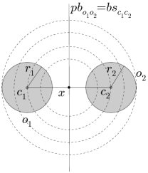
Figure 5: The probabilistic bisector of objects $o_{1}$ and $o_{2}$, where $r_{1}=r_{2}$

Lemmas 4.5 and 4.6 show how the probabilistic bisector of two non-equi-range objects $o_{i}$ and $o_{j}$ is related to the bisector of $c_{i}$ and $c_{j}$ (Figure 6 and  7).

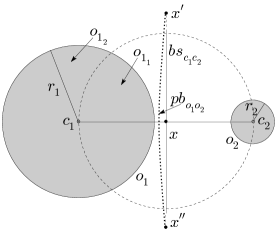
Figure 6: The probabilistic bisector of objects $o_{1}$ and $o_{2}$, where $r_{1}>r_{2}$. The curve, $pb_{{o_{1}}{o_{2}}}$, is the probabilistic bisector between $o_{1}$ and $o_{2}$, i.e., $p(o_{1},x)=p(o_{2},x)$, for any point $x\in\{pb_{{o_{1}}{o_{2}}}\}$

Next, we will show in Lemma 4.5 that the shape of $pb_{o_{i}o_{j}}$ for two non-equi-range circular objects $o_{i}$ and $o_{j}$ is a curve, and the distance of this curve from $bs_{c_{i}c_{j}}$ is maximum on the line $\overline{c_{i}c_{j}}$. Figure 6 shows the bisector $bs_{c_{1}c_{2}}$ and the probabilistic bisector $pb_{o_{1}o_{2}}$ for $o_{1}$ and $o_{2}$.

Lemma 4.5

Let $o_{i}$ and $o_{j}$ be two objects with non-equi-range uncertain circular regions $(c_{i},r_{i})$ and $(c_{j},r_{j})$, respectively, and $bs_{c_{i}c_{j}}$ be the bisector of $c_{i}$ and $c_{j}$. Then the maximum distance between $bs_{c_{i}c_{j}}$ and $pb_{o_{i}o_{j}}$ occurs on the line $\overline{c_{i}c_{j}}$. This distance gradually decreases as we move towards positive or negative infinity along the bisector $bs_{c_{i}c_{j}}$.

Proof 4.5

Let $x=\frac{c_{i}+c_{j}}{2}$ be the intersection point of $bs_{c_{i}c_{j}}$ and $\overline{c_{i}c_{j}}$. Suppose a circle centered at $x$ with radius $\frac{dist(c_{i},c_{j})}{2}$ divides $o_{i}$ into $o_{i_{1}}$ and $o_{i_{2}}$, where $\frac{o_{i_{1}}}{A_{i}}+\frac{o_{i_{2}}}{A_{i}}=1$, and $o_{j}$ into $o_{j_{1}}$ and $o_{j_{2}}$, where $\frac{o_{j_{1}}}{A_{j}}+\frac{o_{j_{2}}}{A_{j}}=1$. According to curvature properties of circles, since $r_{i}>r_{j}$, we have $\frac{o_{i_{1}}}{A_{i}}<\frac{o_{j_{1}}}{A_{j}}$ (in Figure 6, $\frac{o_{1_{1}}}{A_{1}}<\frac{o_{2_{1}}}{A_{2}}$), which intuitively means, $o_{j}$ is a more probable NN than $o_{i}$ to $x$, i.e., $p(o_{j},x)>p(o_{i},x)$. Thus, $x$ needs to be shifted to a point towards $c_{i}$ (along the line $\overline{xc_{i}}$), such that the probabilities of $o_{i}$ and $o_{j}$ being the NNs to the new point become equal.

Suppose a point $x^{\prime}$ is on $bs_{c_{i}c_{j}}$ at the positive infinity. If a circle centered at $x^{\prime}$ goes through the centers of both objects $o_{i}$ and $o_{j}$, then the curvature of the portion of the circle that falls inside an object ($o_{i}$ or $o_{j}$) will become a straight line. This is because, in this case we consider a small portion of the curve of an infinitely large circle. This circle divides both objects $o_{i}$ and $o_{j}$ into two equal parts $o_{i_{1}}=o_{i_{2}}$ and $o_{j_{1}}=o_{j_{2}}$, respectively. Thus, the probabilities of $o_{i}$ and $o_{j}$ being the NNs will approach to being equal at positive infinity, i.e., $p(o_{j},x^{\prime})\approx p(o_{i},x^{\prime})$, for a large values of $dist(x^{\prime},x)$. Similarly, we can show the case for a point $x^{\prime\prime}$ at the negative infinity on $bs_{c_{i}c_{j}}$ (see Figure 6).

Next, we show in Lemma 4.6 that $pb_{o_{i}o_{j}}$ shifts from $bs_{c_{i}c_{j}}$ towards the object with larger radius, and the distance of $pb_{o_{i}o_{j}}$ from $bs_{c_{i}c_{j}}$ widens with the increase of the ratio of two radii (i.e., $r_{i}$ and $r_{j}$). Figure 7 shows an example of this case.

Lemma 4.6

Let $o_{i}$ and $o_{j}$ be two objects with non-equi-range uncertain circular regions $(c_{i},r_{i})$ and $(c_{j},r_{j})$, respectively, and $x=\frac{c_{i}+c_{j}}{2}$ be the midpoint of the line segment $\overline{c_{i}c_{j}}$. If $r_{i}>r_{j}$, then the probabilistic bisector $pb_{o_{i}o_{j}}$ meets $\overline{c_{i}c_{j}}$ at point $x^{\prime}$, where $x^{\prime}$ lies between $x$ and $c_{i}$. If the circular range of $o_{i}$ increases such that $r_{i}^{\prime}>r_{i}$, then the new probabilistic bisector $pb^{\prime}_{o_{i}o_{j}}$ meets $\overline{c_{i}c_{j}}$ at point $x^{\prime\prime}$ , where $x^{\prime\prime}$ lies between $x$ and $c_{i}$, and $dist(x,x^{\prime})<dist(x,x^{\prime\prime})$.

Proof 4.6

Suppose a circle centered at $x$ with radius $\frac{dist(c_{i},c_{j})}{2}$ divides $o_{i}$ into $o_{i_{1}}$ and $o_{i_{2}}$, where $\frac{o_{i_{1}}}{A_{i}}+\frac{o_{i_{2}}}{A_{i}}=1$, and $o_{j}$ into $o_{j_{1}}$ and $o_{j_{2}}$, where $\frac{o_{j_{1}}}{A_{j}}+\frac{o_{j_{2}}}{A_{j}}=1$. According to curvature properties of circles, since $r_{i}>r_{j}$, we have $\frac{o_{i_{1}}}{A_{i}}<\frac{o_{j_{1}}}{A_{j}}$ (in Figure 7, $\frac{o_{1_{1}}}{A_{1}}<\frac{o_{2_{1}}}{A_{2}}$), which intuitively means, $o_{j}$ is a more probable NN than $o_{i}$ to $x$, i.e., $p(o_{j},x)>p(o_{i},x)$. Thus, $x$ needs to be shifted to a point $x^{\prime}$ towards $c_{i}$, such that the probabilities of $o_{i}$ and $o_{j}$ being the NN to $x^{\prime}$ become equal. Let $o_{i}^{\prime}$ be an object, such that $r_{i}^{\prime}>r_{i}$ and $c_{i}^{\prime}=c_{i}$. Then the circle centered at $x$ with radius $\frac{dist(c_{i},c_{j})}{2}$ divides $o^{\prime}_{i}$ into $o^{\prime}_{i_{1}}$ and $o^{\prime}_{i_{2}}$, where $\frac{o^{\prime}_{i_{1}}}{A_{i}^{\prime}}+\frac{o^{\prime}_{i_{2}}}{A_{i}^{\prime}}=1$. Now, we have $\frac{o^{\prime}_{i_{1}}}{A_{i}^{\prime}}<\frac{o_{i_{1}}}{A_{i}}<\frac{o_{j_{1}}}{A_{j}}$. Thus, $x$ needs to be shifted to a point $x^{\prime\prime}$ more towards $c_{i}$, i.e., $dist(x,x^{\prime})<dist(x,x^{\prime\prime})$, such that the probabilities of $o^{\prime}_{i}$ and $o_{j}$ being the NNs become equal at $x^{\prime\prime}$.

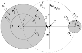
Figure 7: Influence of objects’ sizes on the probabilistic bisector

The next lemma shows the influence of a third object on the probabilistic bisector of two non-equi-range objects. (Note that the probabilistic bisector of two equi-range objects does not change with the influence of any other object (see Lemma 4.4)). Figure 8 shows an example, where object $o_{3}$ influences the probabilistic bisector of objects $o_{1}$ and $o_{2}$. In this figure, the dotted circle centered at $s_{1}$ with radius $dist(s_{1},c_{1})+r_{1}$ encloses one candidate object $o_{1}$, but only touches the third object $o_{3}$. Thus, the probability of $o_{3}$ being the NN to $s_{1}$ is zero. However, for any point between $s_{1}$ and $s_{2}$, $o_{3}$ has a non-zero probability of being the NN of that point, and thus $o_{3}$ influences $pb_{o_{1}o_{2}}$.

Lemma 4.7

Let $o_{i}$ and $o_{j}$ be two objects with non-equi-range uncertain circular regions $(c_{i},r_{i})$ and $(c_{j},r_{j})$, respectively, where $r_{i}<r_{j}$, and $bs_{c_{i}c_{j}}$ be the bisector of $c_{i}$ and $c_{j}$. An object $o_{k}$ influences the probabilistic bisector $pb_{o_{i}o_{j}}$ for the part of the segment $[s_{1},s_{2}]$ on the line $bs_{c_{i}c_{j}}$, where $dist(s,c_{i})+r_{i}>dist(s,c_{k})-r_{k}$ for $s\in bs_{c_{i}c_{j}}$.

Proof 4.7

Since $r_{i}<r_{j}$, we have $maxdist(s,o_{i})<maxdist(s,o_{j})$. Thus, if the minimum distance $mindist(s,o_{k})$ of an object $o_{k}$ from $s$ is greater than the maximum distance $maxdist(s,o_{j})$ of $o_{j}$ from $s$, i.e., $dist(s,c_{k})-r_{k}>dist(s,c_{i})+r_{i}$, the object $o_{k}$ cannot be the NN to the point $s$, otherwise $o_{k}$ has the possibility of being the NN to $s$ and hence $o_{k}$ influences $pb_{o_{i}o_{j}}$.

It is noted when the centers of two non-equal objects coincide each other, the probability of the smaller object dominates the probability of the larger object. Therefore, in those cases, we only consider the object with a smaller radius, and the other object is discarded. Also, if two objects are equal and their centers coincide each other, no probabilistic bisector exists between them, thus any one of these two objects is considered for computing the PVD.

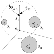
Figure 8: Influence of object $o_{3}$ on the probabilistic bisector of $o_{1}$ and $o_{2}$

Algorithms:

Based on the above lemmas, we propose algorithms to find the probabilistic bisector of any two uncertain 2D objects. We have shown in Lemma 4.4 that the probabilistic bisector of two circular uncertain objects is a straight line when the radii of two objects are equal. On the other hand, Lemma 4.5-Lemma 4.6 show that the probabilistic bisector is a curve when the radii of two objects are non-equal. However, to avoid the computational and maintenance costs, we maintain a bounding box (i.e., quadrilateral) that encloses the actual probabilistic bisector of two objects. Hence, we name the probabilistic bisector of two circular objects as the Probabilistic Bisector Region (PBR). For example, the bounding box that encloses the curve in Figure 6 is the PBR for two objects $o_{1}$ and $o_{2}$. In our algorithm, we first create an ordinary Voronoi diagram by using the centers of all uncertain objects. Then, from each Voronoi edge $e_{ij}$ (i.e., $bs_{c_{i}c_{j}}$) of two objects $o_{i}$ and $o_{j}$, we compute the PBR that encloses $pb_{o_{i}o_{j}}$.

Algorithm 3 computes the probabilistic bisector of two equi-range objects according to Lemma 4.4 (Line 32). Otherwise, it calls the function $FindProbBisector2D$ to determine $pb_{o_{i}o_{j}}$ for two non-equi-range objects $o_{i}$ and $o_{j}$.

if $r_{i}=r_{j}$ then  $pb_{o_{i}o_{j}}\leftarrow ProbBisector(o_{i},o_{j},e_{ij})$ AlgoLine0.0.1

else  $pb_{o_{i}o_{j}}\leftarrow FindProbBisector2D(o_{i},o_{j},e_{ij},O)$ AlgoLine0.0.2

  return $pb_{o_{i}o_{j}}$;

Algorithm 3 ProbBisector2D($o_{i},o_{j},e_{ij},O$)

0.2

0.2

The function $FindProbBisector2D$ (see Algorithm 4) takes two non-equi-range objects $o_{i}$, $o_{j}$, the bisector $e_{ij}$ (i.e., a Voronoi edge) of $c_{i}$ and $c_{j}$, and the set of objects $O$ as input, and returns $pbr$ for $pb_{o_{i}o_{j}}$. The algorithm finds lower ($lval$) and upper ($uval$) bounds representing the required deviations of the probabilistic bisector from the bisector of $c_{i}$ and $c_{j}$, such that the PBR can be computed by drawing two lines parallel to $e_{ij}$ at $lval$ and $uval$, respectively. Algorithm 4 first initializes $ipb$ with the intersection point of $e_{ij}$ and $\overline{c_{i}c_{j}}$ (Line 4.1). Then, the function $InitPBRBound$ computes initial lower ($lval$) and upper ($uval$) bounds of $pbr$ (Line 4.2). This function first determines a point $x^{\prime}$ on the line $\overline{c_{i}c_{j}}$ where $p(o_{i},x^{\prime})\approx p(o_{j},x^{\prime})$ (We use a similar search technique as described for the 1D space).

$ipb\leftarrow Intersect(e_{ij},\overline{c_{i}c_{j}})$AlgoLine0.0.1

$InitPBRBound(lval,hval,ipb)$AlgoLine0.0.2

$IL\leftarrow FindInfluencedPart(o_{i},o_{j},e_{ij})$AlgoLine0.0.3

for each $ls\in IL$ do  $UpdatePBRBound(lval,hval,ls)$ AlgoLine0.0.4

  $pbr\leftarrow[lval,hval]$AlgoLine0.0.5

return $pbr$;

Algorithm 4 FindProbBisector2D($o_{i},o_{j},e_{ij},O$)

If $x^{\prime}$ is to the left of $e_{ij}$, then $lval$ and $hval$ are set to $x^{\prime}$ and $x$, respectively. On the other hand, if $x^{\prime}$ is to the right of $e_{ij}$, then $lval$ and $hval$ are set to $x$ and $x^{\prime}$, respectively. After that, the function $FindInfluencePart$ finds a list $IL$ that contains different segments of the bisector $e_{ij}$, where other objects influence $pb_{o_{i}o_{j}}$ (see Lemma 4.7). The function returns $IL$ as an empty list when no other object influences the probabilistic bisector. In that case the current $lval$ and $hval$ defines $pbr$. In Lemma 4.6, we have seen that the maximum distance of $pb_{o_{i}o_{j}}$ from the bisector of $c_{i}$ and $c_{j}$ is on the line $\overline{c_{i}c_{j}}$. Thus, the initially computed $pbr$ encloses the curve of $pb_{o_{i}o_{j}}$. On the other hand, if $IL$ is not empty, then for each line segment $ls\in IL$, the function $UpdatePBRBound$ is called to update $lval$ and $hval$ based on the influence of other objects. As $lval$ and $hval$ represent the deviation of $pb_{o_{i}o_{j}}$ from $e_{ij}$, we need compute the deviations for each line segment $ls$, and then take the minimum of all $lval$s and the maximum of all $hval$s to compute the $pbr$. To avoid a brute-force approach of computing $lval$ and $hval$ for every point of an $ls\in IL$, we compute $lval$ and $hval$ for two extreme points and the mid-point of $ls$. Finally, the algorithm returns $pbr$ for $pb_{o_{i}o_{j}}$.

0.5

0.5

0.5

0.5

0.5

$PVD\leftarrow\emptyset$AlgoLine0.0.1

$VD\leftarrow VornoiDiagramOfCentroids(O)$AlgoLine0.0.2

AlgoLine0.0.3

for each Voronoi edge $e_{ij}\in VD$, where $o_{i},o_{j}\in O$ do  $PVD\leftarrow PVD\cup ProbBisector2D(o_{i},o_{j},e_{ij},O)$ AlgoLine0.0.4

  return $PVD$;

Algorithm 5 ProbVoronoi2D(O)

0.4

0.4

0.4

0.4

Algorithm 5 shows the steps of $ProbVoronoi2D$ that computes $PVD$ for a given set $O$ of 2D objects. In Line 5.2, the algorithm first creates a Voronoi diagram $VD$ for all centers $c_{i}$ of objects $o_{i}\in O$ using [22]. Then for each Voronoi edge $e_{ij}$ between two objects $o_{i}$ and $o_{j}$, the algorithm calls the function $ProbBisector2D$ to compute the probabilistic bisector as PBR between two candidate objects, and finally it returns the PVD for the given set $O$ of objects.

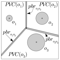
Figure 9: The PVD of three objects $o_{1}$, $o_{2}$, and $o_{3}$

Figure 9 shows the PVD for objects $o_{1}$, $o_{2}$, and $o_{3}$. In this figure, $PVC(o_{1})$, $PVC(o_{2})$, and $PVC(o_{3})$ represent the PVCs for objects $o_{1}$, $o_{2}$, and $o_{3}$, respectively. The boundaries between PVCs, i.e., PBRs of objects, $pbr_{o_{1}o_{2}}$, $pbr_{o_{2}o_{3}}$, and $pbr_{o_{1}o_{3}}$, are shown using grey bounded regions. For any point inside a PVC, the corresponding object is guaranteed to be the most probable NN. On the other hand, for any point inside a PBR, any of the two objects that share the PBR can be the most probable NNs. If more than two PBRs intersect each other in a region, any object associated with these PBRs can be the most probable NN to a query point in that region. Figure 9 shows a dark grey region where $pbr_{o_{1}o_{2}}$, $pbr_{o_{1}o_{3}}$, and $pbr_{o_{2}o_{3}}$ meets.

Complexity: The complexity of Algorithm 5 can be estimated as follows. The complexity of creating a Voronoi diagram (Line 5.2) is $O(n\log n)$ [22], where $n$ is the number of objects. The complexity of finding probabilistic bisectors (Lines 5.3-5.4) is $O(n_{e}C_{pb})$, where $n_{e}$ is the number of Voronoi edges and $C_{pb}$ is the expected cost of computing the probabilistic bisector between two circular objects. For real data sets, $n_{e}$ is expected to be a small integer since an object has only a small number of surrounding objects. The total complexity of the algorithm is $O(n\log n)$+$O(n_{e}C_{pb})$. $C_{pb}$ can be estimated as follows. Let $C_{b}$ be the cost of computing the probability of an object being the NN of a query point, $D$ be the expected distance between the initial probabilistic bisector $ipb$ and the actual probabilistic bisector, and $L$ be the expected number of points in the bisector that needs to be considered to find upper and lower bounds of the probabilistic bisector. Then we have $C_{pb}=O(LC_{b}\log_{2}D)$. This is because, the cost of finding a probabilistic bisector is $O(1)$ for the cases when our algorithm can directly compute the probabilistic bisector, and for other cases our algorithm first finds $ipb$ by $O(1)$ and then search for the actual probabilistic bisector by using Algorithm 4 by $O(L\log D)$. Note that, for both 1D and 2D, the run-time behavior of our algorithm is dominated by those cases for which there is no closed form for a given probabilistic bisector, i.e., the algorithm needs to search for the bisector by using the initial probabilistic bisector.

4.3 Discussion

PVD for Other Distributions: In this paper, we assume the uniform distributions for the pdf of uncertain objects to illustrate the concept of the PVD. However, the pdf that describes the distribution of an object inside the uncertainty region can follow arbitrary distributions, e.g., Gaussian. The concept of PVD can be extended for any arbitrary distribution. For example, for an object with Gaussian pdf having a circular uncertain region, the probability of the object of being around the center of the circular region is higher than that of the boundary region of the circle. For such distributions, a straightforward approach to compute the probabilistic bisector between any pair of objects is as follows. First, we can use the bisector of the centroids of two candidate objects as the initial probabilistic bisector. Then we can refine the initial probabilistic bisector to find the actual probabilistic bisector. Finding suitable initial probabilistic bisectors for efficient computation of probabilistic bisectors (e.g., lemmas for different cases for 1D and 2D data sets similar to the uniform pdf) for an arbitrary distribution is the scope of future investigation.

PVD for Higher Dimensions: We can compute the PVD for higher dimensional spaces, similar to 1D and 2D spaces. For example, in a 3D space, an uncertain object can be represented as a sphere instead of a circle in 2D. Then, the probabilistic bisector of two equal size spheres will be a plane bisecting the centers of two spheres. Using this as a base, similar to 2D, we can compute the PVD for 3D objects. We omit a detailed discussion on PVDs in spaces of more than 2 dimensions.

Higher order PVDs: In this paper, we focus on the first order PVD. By using this PVD, we can find the NN for a given query point. Thus, the PVD can be used for continuously reporting 1-NN for a moving query point. To generalize the concept for $k$NN queries, we need to develop the $k$-order PVD. The basic idea would be to find the probabilistic bisectors among size-$k$ subsets of objects. The detailed investigation of higher order PVDs is a topic of future study.

Handling Updates: To handle updates on the data objects, like traditional Voronoi diagrams, a straightforward approach is to recompute the entire PVD. There are algorithms [23, 24] to incrementally update a traditional Voronoi diagram. Similar ideas can be applied to the PVD to derive incremental update algorithms. We will defer such incremental update algorithms for future work.

It is noted that, to avoid an expensive computation of the PVD for the whole data set and to cope with updates for the data objects, we propose an alternative approach based on the concept of local PVD (see Section 5.5.2). In this approach, only a subset of objects that fall within a specified range of the current position of the query is retrieved from the server and then the local PVD is created for these retrieved objects to answer PMNN queries. If there is any update inside the specified range, the process needs to be repeated. Since, this approach works only with the surrounding objects of a query, updates from objects that are outside the range do not affect the performance of the system.

5 Processing PMNN Queries

In this section, based on the concept of PVD we propose two techniques: a pre-computation approach and an incremental approach for answering PMNN queries. In the pre-computation approach, we first create the PVD for the whole data set and then index the PVCs for answering PMNN queries. We name the pre-computation based technique for processing PMNN queries as P-PVD-PMNN. On the other hand, in the incremental approach, we retrieve a set of surrounding objects with respect the current query location and then create the local PVD for these retrieved data set, and finally use this local PVD to answer PMNN queries. We name this approach I-PVD-PMNN in this paper.

5.1 Pre-computation Approach

In the pre-computation approach, we first create the PVD for all objects in the database. After computing the PVD, we only need to determine the current Probabilistic Voronoi Cell (PVC), where the current query point is located. The query evaluation algorithm can be summarized as follows.

Initially, the query issuer requests the most probable NN for the current query position $q$. After receiving the PMNN request for $q$, the server algorithm finds the current PVC to which the query point falls into using a function $IdentifyPVC$ and updates $cpvc$ with the current PVC. The algorithm reports the corresponding object $p$ as the most probable NN and the cell $cpvc$ to the query issuer. Next time when $q$ is updated at the query issuer, if $q$ falls inside $cpvc$, no request is made to the server as the most probable NN has not been changed. Otherwise, the query issuer again sends the PMNN request to the server to determine the new PVC and the answer for the updated query position.

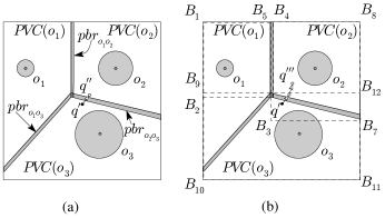
Figure 10: (a) The PVD, and (b) the MBRs of PVCs for objects $o_{1}$-$o_{3}$

As the PVD in a 1D space contains a set of non-overlapping ranges representing PVCs for objects, the algorithm returns a single object as the most probable NN for any query point. On the other hand, in a 2D space, the boundary between two PVCs is a region (i.e., PBR) rather than a line. When a query point falls inside a PBR, the algorithm can possibly return both objects that share the PBR as the most probable NNs, or preferably can decide the most probable NN by computing a top-1-PNN query. (Since, for a realistic setting a PBR is small region compared to that of PVCs, our approach incurs much less computational overhead than that of the sampling based approach for processing a PMNN query.)

Figure 10(a) shows that when the query point is at $q^{\prime}$, PVD-PMNN returns $o_{3}$ as the most probable NN as $q^{\prime}$ falls into PVC($o_{3}$). When the query point moves to $q^{\prime\prime}$, the algorithm returns $o_{2}$ as the answer.

A naive approach of identifying the desired PVC (i.e., $IdentifyPVC$ function) requires an exhaustive search of all the PVCs in a PVD, which is an expensive operation. Indexing Voronoi diagrams [25, 26, 27] is an well-known approach for efficient nearest neighbor search in high-dimensional spaces. Thus, for efficient search of the PVCs, we index the PVCs of the PVD using an $R^{*}$-tree [28], a variant of the $R$-tree [29, 27]. In a 1D space, each PVC is represented as a 1D range and is indexed using a 1D $R^{*}$-tree. Since there is no overlap among PVCs, a query point always falls inside a single PVC, where the corresponding object is the most probable NN to the query point. On the other hand, in a 2D space, each PVC cell is enclosed using a Minimum Bounding Rectangle (MBR), and is indexed using a 2D $R^{*}$-tree. Since the MBRs representing PVCs overlap each other, when a query point falls inside only a single MBR, the corresponding object is confirmed to be the most probable NN to the query point. However, when a query point falls inside the overlapping region of two or more MBRs, the actual most probable NN can be identified by checking the PVCs of all candidate MBRs. Figure 10(b) shows the MBRs $[B_{1},B_{2},B_{3},B_{4}]$, $[B_{5},B_{6},B_{7},B_{8}]$, and $[B_{9},B_{10},B_{11},B_{12}]$ for the PVCs of objects $o_{1}$, $o_{2}$, and $o_{3}$, respectively. In this example, the query point $q^{\prime}$ intersects both $[B_{5},B_{6},B_{7},B_{8}]$ and $[B_{9},B_{10},B_{11},B_{12}]$, and the actual most probable NN $o_{3}$ can be determined by checking the PVCs of $o_{3}$ and $o_{2}$; on the other hand, the query point $q^{\prime\prime\prime}$ only intersects a single MBR $[B_{5},B_{6},B_{7},B_{8}]$, so the corresponding object $o_{2}$ is the most probable NN to $q^{\prime\prime\prime}$.

Since the above approach only retrieves the current PVC of a moving query point, it needs to access the PVD using the $R^{*}$-tree as soon as the query leaves the current PVC. This may incur more I/O costs than what can be achieved. To further reduce I/O and improve the processing time, we use a buffer management technique, where instead of only retrieving the PVC that contains the given query point, we retrieve all PVCs whose MBRs intersect with a given range, called a buffer window, for a given query point. These PVCs are buffered and are used to answer subsequent query points of a moving query. This process is repeated for a PMNN query when the buffered cells cannot answer the query.

Since the creation of the entire PVD is computationally expensive, the pre-computation based approach is justified when the PVD can be re-used which is the case for static data, or when the query spans over the whole data space. To avoid expensive pre-computation, next, we propose an incremental approach which is preferable when the query is confined to a small region of the data space or when there are frequent updates in the database.

5.2 Incremental Approach

In this section, we describe our incremental evaluation technique for processing a PMNN query based on the concept of known region and the local PVD. Next, we briefly discuss the concept of known region, and then present the detailed algorithm of our incremental approach.

Known Region: Intuitively, the known region is an explored data space where the position of all objects are known. We define the known region as a circular region that bounds the top-$k$ probable NNs with respect to the current query point (i.e., the center point of the region). For a given point $q_{s}$, the server expands the search space to incrementally access objects in the order of their $mindist$ from $q_{s}$ until it finds top $k$ probable nearest neighbors with respect to $q_{s}$ (we use existing algorithm [8] to find top-$k$NN). Then the known region is determined by a circular region centered at $q_{s}$ that encloses all these $k$ objects. Figure 11 shows the known circular region $K(q_{s},r)$ using a dashed circle, where $k=3$. Then the radius $r$ of this known area is determined by $max(maxdist(q_{s},o_{1}),maxdist(q_{s},o_{2}),maxdist(q_{s},o_{3}))$. In this example, top-3 most probable nearest neighbors are $o_{1}$,$o_{2}$, and $o_{3}$.

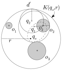
Figure 11: Known region and objects $o_{1}$, $o_{2}$, and $o_{3}$

The key idea of incremental approach is to consider only a sub-set of objects surrounding the moving query point while evaluating a PMNN query. For example, in a client-server paradigm, the client first requests the server for objects and the known region by providing the starting point of the moving query path as a query point. Then the client locally creates a PVD based on the retrieved objects, and uses the local PVD for answering the PMNN query. This process needs to be repeated as soon as the user’s request for the PMNN query cannot be satisfied by the already retrieved data at the client. Though this incremental approach applies to both centralized and client-server paradigms, without loss of generality, next we explain how to incrementally evaluate a PMNN query in the client-server paradigm.

Algorithm: After retrieving a set of objects from the server, the client locally computes a PVD for those objects. Then, the client can use the local PVD to determine the most probable nearest neighbor among the objects inside the known region. However, since the client does not have any knowledge about objects that are outside of the known region, the most probable nearest neighbor based on the local PVD formed for objects inside the known region, might not guarantee the most probable nearest neighbor with respect to all objects in the database. This is because, a PVC of the local PVD determines the region where the corresponding object is the most probable NN with respect to objects inside the known region. However, certain locations of the PVC can have other non-retrieved objects, which are outside the known region, as the most probable NN. Thus, we need to determine a region in the PVC for which the query result is guaranteed. That is, all locations inside this guaranteed region will have the corresponding object as the most probable NN. To define the guaranteed region for an object, we have two conditions.

Let $q$ be a query point and $o_{i}$ be an object inside the known region. Then, if the query point $q$ is inside a PVC cell of object $o_{i}$ and the condition in the following equation (see Equation 2) holds, then it is ensured that $o_{i}$ is the most probable NN among all objects in the database.

$$maxdist(q,c_{i})\leq r-dist(q,q_{s}).$$ (2)

The condition in Equation 2 ensures that no object outside the known region can be the nearest neighbor for the given query point. This is because, when a circle centered at $q$ completely contains an object, all objects outside this circle will have zero probability of being the NN to $q$.

To formally define a region based on the above inequality, we re-arrange Equation 2 as follows.

$$dist(q,c_{i})+r_{i}\leq r-dist(q,q_{s})$$

$$=>dist(q,c_{i})+dist(q,q_{s})\leq r-r_{i}$$

We can see that the boundary of the above formula forms an elliptic region in a 2D Euclidean space, where the two foci of the ellipse are $q_{s}$ and $c_{i}$. i.e., the sum of the distances from $q_{s}$ and $c_{i}$ to any point on the ellipse is $r-r_{i}$. Figure 11 shows an example, where the elliptical region for object $o_{2}$ is shown using dashed border. Figure 11 shows that when the query point is at $q_{1}$, the object $o_{2}$ is confirmed to be the most probable nearest neighbor, as $dist(q_{1},c_{2})+r_{2}<r-dist(q_{1},q_{s})$.

From the above discussion, we see that for an object $o_{i}$, the intersection region of the PVC and the elliptical region for $o_{i}$ forms a region where all points in this region has $o_{i}$ as the most probable NN. Figure 12 shows the PVD and elliptical regions for objects $o_{1}$, $o_{2}$, and $o_{3}$, and a moving query path from $q^{\prime}$ to $q^{\prime\prime\prime}$. In this figure, since $q^{\prime}$ is inside the intersection region of $PVC(o_{3})$ and elliptical region of $o_{3}$, thus $o_{3}$ is guaranteed to be the most probable NN for $q^{\prime}$ with respect to all objects in the database. Similarly, $o_{2}$ is the most probable NN when the query point moves to $q^{\prime\prime\prime}$.

If a query point is outside the intersection region of a PVC and the corresponding elliptical region, but falls inside the PVC, still there is a possibility that the object associated with this PVC is the most probable NN for the query point. For example, in Figure 11, when the query point is at $q_{2}$, then the condition in Equation 2 fails. For this case, our algorithm relies on the lower bound of the probability for the object $o_{2}$ of being the nearest neighbor from the query point $q_{2}$. We define the second condition based on the lower bound probability of an object.

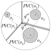
Figure 12: The incremental approach

We can compute the lower bound of probability, $lp(o_{i},q)$ for object $o_{i}$ of being the NN from the query point $q$, by using pessimistic assumption. For computing the lower bound probability, we assume that a non-retrieved virtual point object is located at the minimum distance from the query point and is just outside the boundary surface of the known region. For example, in Figure 11, when the client is at $q_{2}$, we assume that a point object exists at $d^{\prime}$. Then, we estimate the probability of the object $o_{2}$ being the NN to $q_{2}$, which gives us the lower bound of the probability.

By using the lower bound, the client can determine whether there is a possibility of other non-retrieved objects being the most probable NN from the current query location. If the probability of the virtual point object $o_{v}$, $p(o_{v},q)$ is less than the lower bound probability of the candidate object $o_{i}$, $lp(o_{i},q)$, then it is ensured that there is no other object in the database that has higher probability for being the NN of $q$ than that of $o_{i}$; otherwise there may exist other object in the database with higher probabilities for being the NN of $q$ than $o_{i}$. Thus, our second condition for the guaranteed region can be defined as follows:

$$lp(o_{i},q)\geq p(o_{v},q).$$ (3)

Based on the above observations, we define a probabilistic safe region for an object $o_{i}$, as a region where $o_{i}$ is guaranteed to be the most probable NN for every point inside that region. Thus, Equation 2 and Equation 3 form the guaranteed region for an object $o_{i}$.

We use the above two conditions and the local PVD to incrementally evaluate a PMNN query. The algorithm first retrieves a set of surrounding objects for the given query point $q$, and creates a PVD, named $lPVD$, for those objects. Then, the algorithm finds the PVC and the corresponding object $o_{i}$ as the most probable nearest neighbor of the query point $q$ with respect to the objects within the known region. If $q$ is inside a PVC cell, the object $o_{i}$ is returned as the most probable nearest neighbor if $q$ satisfies Equation 2 or Equation 3. If none of the above condition holds, the algorithm requests a new set of objects with respect to the current query point $q$, and repeats the above process on newly retrieved set of objects.

Discussion: Our pre-computation based approach computes the PVD for all objects in the database and then indexes the PVD using an $R$-tree to efficiently process PMNN queries. Since, the pre-computation of the PVD for the entire data set is computationally expensive, the pre-computation based approach is justified when the PVD can be re-used for large number of queries, as the cost is amortized among queries(e.g., [11, 20]). Thus, the pre-computation based approach is appropriate for the following settings: the data set largely remains static, there are large number of queries in the system, and the query spans over the whole data space.

On the other hand, in our incremental approach, we retrieve a set of surrounding objects for the current query location, and then incrementally process PMNN queries based only on these retrieved set of objects. Only data close to the given query are accessed for query evaluation. As the evaluation of this approach depends on the location of the query, this approach is also called the query dependent approach, as opposed to the data dependent approach (e.g., pre-computation based approach) where the location of queries are not taken into account. This incremental approach is preferred for the cases when there are updates in the database or the query is confined to a small region in the data space. A comparative discussion between the pre-computation approach and the incremental approach for point data sets can be found in [30, 20].

6 Experimental Study

We compare our PVD based approaches for the PMNN query (P-PVD-PMNN and I-PVD-PMNN) with a sampling based approach (Naive-PMNN), which processes a PMNN query as a sequence of static PNN queries at sampled locations. Though in Naive-PMNN we use the most recent technique of static top-1-PNN queries [8], any existing technique for static PNN queries [4, 5] can be used. Note that, by using the existing method in [6], for each uncertain object $o_{i}$, we could only define a region (or UV-cell) where $o_{i}$ has a non-zero probability of being the NN for any point in this region. Thus, this method cannot be used to determine whether an object has the highest probability of being the NN to a query point. Therefore, we compare our approach with a sampling based approach.

In our experiments, we measure the query processing time, the I/O costs, and the communication costs as the number of communications between a client and a server. Note that while the processing and I/O costs are the performance measurement metric for both centralized and client-server paradigms, the communication cost only applies to the client-server paradigm. In this paper, we run the experiments in the centralized paradigm, where the query issuer and the processor reside in the same machine. Thus, we measure the communication cost as the number of times the query issuer communicates with the query processor while executing a PMNN query.

6.1 Experimental Setup

We present experimental results for both 1D and 2D data sets.

For 2D data, we have used both synthetic and real data sets. We normalize the data space into a span of $10,000\times 10,000$ square units. We generated synthetic data sets with uniform (U) and Zipfian (Z) distributions, representing a wide range of real scenarios. For both uniform and Zipfian, we vary the data set size from 5K to 25K. To introduce uncertainty in data objects, we randomly choose the uncertainty range of an object between $5\times 5$ and $30\times 30$ square units, and approximated the selected range using a circle. For real data distributions, we use the data sets from Los Angeles (L) with 12K geographical objects described by ranges of longitudes and latitudes [31]. Note that, in both uniform and Zipfian distributions, objects can overlap each other. More importantly, in Zipfian distribution, most of the objects are concentrated within a small region in the space, thereby objects largely overlap with each other. Also, our real datasets include objects with large and overlapping regions. Thus, we do not present any sperate experimental results for overlapping objects.

For 1D data, we have only used syntectic data sets. In this case, we generated synthetic data sets with uniform (U) and Zipfian (Z) distributions in the data space of 10,000 units. The uncertainty range of an object is chosen as any random value between 5 and 30 units. We also vary the data set size from 100 to 500. These values are comparable to 2D data set sizes and scenarios.

For query paths, we have generated two different types of query trajectories, random (R) and directional (D), representing the query movement paths covering a large number of real scenarios. The default length of a trajectory is a fixed length of 1000 steps, and consecutive points are connected with a straight line of a length of 5 units. For each type of query path, we run the experiments for 20 different trajectories starting at random positions in the data space, and determine the average results. We present the processing time, I/O cost, and the communication cost for executing a complete trajectory (i.e., a PMNN query). In our experiments, since the trajectory of a moving query path is unknown, we use the generated trajectories as input, but do not provide these to the server in advance.

We run the experiments on a desktop computer with Intel(R) Core(TM) 2 CPU 6600 at 2.40 GHz and 2 GB RAM.

6.2 Performance Evaluation

In this section, we evaluate our proposed techniques: pre-computation approach (P-PVD-PMNN) and incremental approach (I-PVD-PMNN) in Sections 6.2.1 and 6.2.2, respectively.

It is well known that pre-computation based approach is suitable for settings when the PVD can be re-used (e.g., static data sets) for large number of queries or the query span the whole data space, and on the other hand the incremental or local approach is suitable for settings when the query is confined to a small space and there are frequent updates in the database (e.g., [30, 11, 20]). Since two approaches aim at two different environmental settings and also the parameters of these two techniques differ from each other, we independently evaluate them and compare them with the sampling based approach.

6.2.1 Pre-computation Approach

In the pre-computation approach, we first create the PVD for the entire data set and use an $R^{*}$-tree to index the MBRs of PVCs. On the other hand, for Naive-PMNN we use an $R^{*}$-tree to index uncertain objects. In both cases, we use the page size of 1KB and the node capacity of 50 entries for the $R^{*}$-tree.

Experiments with 2D Data Sets:

We vary the following parameters in our experiments: the length of a query trajectory, the data set size, and the size of the buffer window that determines the number of PVCs retrieved each time with respect to a query point.

Effect of the Length of a Query Trajectory: In this set of experiments, we vary the length of moving queries from 1000 to 5000 units of the data space. We run the experiments for data sets U(10K), Z(10K), and L(12K). Since the real data set size is 12K, the data set sizes for U and Z are both set to 10K. Figures 13 show the processing time, I/O costs, and the number of communications required for a PMNN query of different query trajectory length. Figures 13(a)-(c) present the results for U data sets, where we can see that, for both P-PVD-PMNN and Naive-PMNN, the processing time, I/O costs, and the number of communications increase with the increase of the length of the query trajectory, which is expected. Figures also show that our P-PVD-PMNN approach outperforms the Naive-PMNN by at least an order of magnitude in all metrics. This is because, P-PVD-PMNN only needs to identify the current PVC rather than computing top-1-PNN for every sampled location of the moving query.

The results for both Z (see Figures 13(d)-(f)) and L (see Figures 13(g)-(i)) data sets show similar trends with U data set as described above.

(a)	(b)	(c)

(d)	(e)	(f)

(g)	(h)	(i)

Figure 13: The effect of the query trajectory length in U (a-c), Z (d-f), and L (g-i)

(a)	(b)	(c)

(d)	(e)	(f)

Figure 14: The effect of the data set size in U (a-c), Z (d-f)

Effect of Data Set Size: In this set of experiments, we vary the data set size from 5K to 25K and compare the performance of our P-PVD-PMNN with Naive-PMNN for both U (see Figures 14(a)-(c)) and Z (see Figures 14(d)-(f)) distributions. In these experiments, we set the trajectory length to 5000 units.

Figures 14(a)-(f) show that, in general for P-PVD-PMNN, the processing time and I/O costs, and the number of communications increase with the increase of the data set size. The reason is as follows. For a larger data set, since the density of objects is high, we have smaller PVCs. Thus, for a larger data set, as the query point moves, it crosses the boundaries of PVCs more frequently than that of a smaller data set. This operation incurs extra computational overhead for a larger data set. On the other hand, for Naive-PMNN, the processing time, I/O costs, and the communication costs remain almost constant with the increase of the data set size. This is because, unless the $R^{*}$-tree has a new level due to the increase of the data set size, the processing costs for Naive-PMNN do not vary with increase of the data set size, which is the case in Figures 14(a)-(f)).

Figures also show that our P-PVD-PMNN outperforms Naive-PMNN by an order of magnitude in processing time, 2 orders of magnitude in I/Os and number of communications for all data sets. The results also show that P-PVD-PMNN performs similar for both directional (D) and random (R) query movement paths.

(a)	(b)	(c)

(d)	(e)	(f)

(g)	(h)	(i)

Figure 15: The effect of buffer window in U (a-c), Z (d-f), and L (g-i)

Effect of Buffer Window: In this set of experiments, we study the impact of introducing a buffer for processing a PMNN query. We vary the value of buffer window from 0 to 400 units of the data space, and then run the experiments for data sets U(10K), Z(10K), and L(12K). We set the trajectory length to 5000 units.

In these experiments, all PVCs whose MBRs intersect with a buffer window centered at $q$ having the length and width of the buffer window are retrieved from the $R^{*}$-tree and sent to the client. The client stores these PVCs in its buffer. When buffer window is 0, the algorithm only retrieves those PVCs whose MBRs contain the given query point. On the other hand, when buffer window is 100, all PVCs whose MBRs intersect with the buffer window centered at $q$ having the length and width of 100 units (i.e., the buffer window covers $100\times 100$ square units in the data space) are retrieved. In this setting, we expect that the I/O costs will be reduced for a larger value of buffer window, because the server does not need to access the $R^{*}$-tree as long as these buffered PVCs can serve the subsequent query points of a moving query.

Figures 15(a)-(c) show the processing time, the I/O costs, and the number of communications, respectively, for varying the size of the buffer window from 0 to 400 units for U data set. Figure 15(a) shows that for P-PVD-PMNN, in general the processing time increase with increase of buffer window. The reason is that for a very large buffer window, a large number of PVCs are buffered and the processing time increases as the algorithm needs to check these PVCs for a moving query. On the other hand, Figure 15(b) shows that for P-PVD-PMNN, I/O costs decrease with the increase of the buffer window. This is because, for a larger value of buffer window the algorithm fetches more PVCs at a time from the server, and thereby needs to access the PVD using the $R^{*}$-tree reduced number of times. The figure also shows that P-PVD-PMNN outperforms Naive-PMNN by an order of magnitude in processing time and 2 orders of magnitude in I/O. Figure 15(c) shows that the number of communications for P-PVD-PMNN continuously decreases with the increase of buffer window as the client fetches more PVCs at a time from the server. However, for Naive-PMNN, the client communicates with the server for each sampled location of the query, and thus the number of communications remain constant.

The results on Z (see Figures 15(d)-(f)) and L (see Figures 15(g)-(i)) data sets show similar trends with U data set described above.

(a)	(b)	(c)

(d)	(e)	(f)

Figure 16: The effect of the query trajectory length in U (a-c), Z (d-f) for 1D data

(a)	(b)	(c)

(d)	(e)	(f)

Figure 17: The effect of the data set size in U (a-c), Z (d-f) for 1D data

(a)	(b)	(c)

(c)	(d)

Figure 18: The effect of buffer window in U (a-c), Z (d-f) for 1D data

Experiments with 1D Data Sets:

For 1D data, we have run a similar set of experiments to 2D ones, where we vary the length of the query trajectory, the data set size, and the size of the buffer window.

Effect of the Length of a Query Trajectory: In this set of experiments, we vary the query trajectory length from 1000 to 5000 units while evaluating a PMNN query for 1D data sets. We run the experiments for both U (see Figures 16(a)-(c)) and Z (see Figures 16(d)-(f)) data sets. The data set size is set to 100. We can see that, for both P-PVD-PMNN and Naive-PMNN, the processing time, I/O costs, and number of communications increase with the increase of the query trajectory length for 1D sets, which is expected. Figures also show that our P-PVD-PMNN outperforms the Naive-PMNN by at least an order of magnitude in terms of processing time, I/Os, and communication costs.

Effect of Data Set Size: We also run the experiments with varying data set size (see Figures 17(a)-(c) for U and Figures 17(d)-(f) for Z data sets). In these experiments, the trajectory length is set to 5000 units. Figures show that, for P-PVD-PMNN, the processing time, I/O costs and number of communications increase with the increase of data set size for 1D sets. This is because, for a larger data set, we have smaller PVCs and thereby a moving query needs to check higher number of PBRs than that of a smaller data set. Figures 17(a)-(f) also show that our P-PVD-PMNN outperforms Naive-PMNN by at least an order of magnitude in all evaluation metrics. The results also show that P-PVD-PMNN performs similar for both directional (D) and random (R) query movement paths.

Effect of Buffer Window: In this set of experiments, we study the impact of introducing a buffer for processing a PMNN query. We vary the value of buffer window from 0 to 400 units, and then run the experiments for U (see Figures 18(a)-(c)) and Z (see Figures 18(d)-(f)) data sets. In these experiments, we set the data set size to 100 and the trajectory length to 5000 units. The experimental results show that P-PVD-PMNN outperforms Naive-PMNN by 1-2 orders of magnitude for I/O and processing costs, and 2-3 orders of magnitude in terms of communication costs.

6.2.2 Incremental Approach

In the incremental approach, we use an $R^{*}$-tree to index the MBRs of uncertain objects, for both I-PVD-PMNN and Naive-PMNN. In both cases, we use the page size of 1KB and the node capacity of 50 entries for the $R^{*}$-tree.

(a)	(b)	(c)

(d)	(e)	(f)

(g)	(h)	(i)

Figure 19: The effect of (k) in U (a-c), Z (d-f), and L (g-i)

Experiments with 2D Data Sets:

We vary the following parameters in our experiments: the value of $k$ (i.e., the number of objects retrieved at each step), the data set size, and the length of the query trajectory, and compare the performance of I-PVD-PMNN with Naive-PMNN.

Effect of $k$: In this set of experiments, we study the impact of $k$ in the performance measure for processing a PMNN query. We vary the value of $k$ from 10 to 50, and then run the experiments for all available data sets (U, Z, and L). In these experiments, for both U and Z, we have set the data set size to 10K. Figures 19(a)-(c) show the processing time, the I/O costs, and the number of communications, respectively, for varying $k$ from 10 to 50 for U data set. Figure 19(a) shows that the processing time almost remains constant for varying $k$. The processing time of I-PVD-PMNN is on average 6 times less for directional (D) query paths than that of Naive-PMNN, and on average 13 times less for random (R) query paths than that of Naive-PMNN. On the other hand, Figures 19(b)-(c) show that I/O costs and the number of communications decrease with the increase of $k$. This is because, for a larger value of $k$, the client fetches more data at a time from the server, and thereby needs to communicate less number of times with the server. Figures also show that our I-PVD-PMNN outperforms the Naive-PMNN by 2-3 orders of magnitude for both I/O and communication costs.

Figures 19(d)-(f) and (g)-(i) show the performance behaviors of Z and L data sets, respectively, which are similar to U data set.

(a)	(b)	(c)

(d)	(e)	(f)

Figure 20: The effect of the data set size in U (a-c), Z (d-f)

(a)	(b)	(c)

(d)	(e)	(f)

Figure 21: The effect of the query length in U (a-c), Z (d-f)

Effect of Data Set Size: In this set of experiments, we vary the data set size from 5K to 25K and compare the performance of our approach I-PVD-PMNN with Naive-PMNN. We set the trajectory length to 5000 units. Also, in these experiments, we have set the value of $k$ to 30. Figures 20 (a)-(c) and (d)-(f) show the processing time, I/O costs, and the number of communications for U and Z data sets, respectively. Figures also show that our I-PVD-PMNN outperforms Naive-PMNN by 1-3 orders of magnitude for all data sets.

Effect of the Length of a Query Trajectory: We vary the length of moving queries from 1000 to 5000 units of the data space. In these experiments, for both U and Z, we have set the data set size to 10K. Also, in these experiments, we have set the value of $k$ to 30. Figures 21 show that the processing time, I/O costs, and the number of communications increase with the increase of the length of the query trajectory for both U and Z data sets, which is expected. The processing time of I-PVD-PMNN is on average 5 times less for directional (D) query path and is on average 10 times less for random (R) query paths compared to Naive-PMNN. Also I-PVD-PMNN outperforms Naive-PMNN by at least an order of magnitude for both I/O and communication costs.

(a)	(b)	(c)

(d)	(e)	(f)

Figure 22: The effect of (k) in U (a-c), Z (d-f) for 1D data

(a)	(b)	(c)

(d)	(e)	(f)

Figure 23: The effect of the data set size in U (a-c), Z (d-f) for 1D data

Experiments with 1D Data Sets: We also evaluate our incremental approach with 1D data sets by varying the following parameters: the value of $k$, the data set size, and the length of the query trajectory.

Effect of $k$: In this set of experiments, we study the impact of $k$ in the performance measure of I-PVD-PMNN for 1D data sets. Figures 22(a)-(e) show the results of U and Z data sets, for varying $k$ from 10 to 50. In these experiments, we have set the data set size to 100. Figure 22(a) shows that the processing time almost remains constant for varying $k$. Moreover, the processing time of I-PVD-PMNN is on average 6 times less for directional (D) query paths than that of Naive-PMNN, and on average 10 times less for random (R) query paths than that of Naive-PMNN. Figures 22(b)-(c) show that the I/O costs and the number of communications decrease with the increase of $k$. Figures also show that our I-PVD-PMNN outperforms Naive-PMNN by 2-3 orders of magnitude in terms of both I/O costs and communication costs.

Figures 22(d)-(f) show the results for Z data set, which is similar to U data set.

Effect of Data Set Size: In this set of experiments, we vary the data set size from 100 to 500 and compare the performance of our approach I-PVD-PMNN with Naive-PMNN. In these experiments, we have set the value of $k$ to 30 and the trajectory length to 5000 units. Figures 20 (a)-(c) and (d)-(f) show the processing time, I/O costs, and the number of communications for U and Z data sets, respectively. The results reveal that the processing time, I/O costs, and the communications costs increase with the increase of the data set size. Figures also show that our I-PVD-PMNN outperforms Naive-PMNN by at least an order of magnitude for all data sets.

(a)	(b)	(c)

(d)	(e)	(f)

Figure 24: The effect of the query length in U (a-c), Z (d-f) for 1D data

Effect of the Length of a Query Trajectory: We also vary the length of the query trajectory for 1D data sets and the results (Figures 24) for 1D data sets exhibit similar behavior to 2D data sets. In these experiments, we vary the trajectory length from 1000 to 5000 units of the data space. Also, we have set the data set size to 100, and the value of $k$ to 30. Figures 24 show that for both U and Z data sets, the processing time, I/O costs, and the communication costs increase with the increase of the trajectory length. Figures also show that our I-PVD-PMNN outperforms Naive-PMNN in all evaluation metrics.

7 Summary

In this paper, we have introduced the concept of Probabilistic Voronoi Diagrams (PVDs). A PVD divides the data space using a probability measure. Based on the PVD, we developed two different techniques: a pre-computation approach and an incremental approach, for efficient processing of Probabilistic Moving Nearest Neighbor (PMNN) queries. Our experimental results show that our techniques outperform the sampling based approach by up to two orders of magnitude in our evaluation metrics.

Our work on PVD opens new avenues for future work. Currently our approach finds the most probable NN for a moving query point; in the future we aim to extend it for top-$k$ most probable NNs. PVDs for other types of probability density functions such as normal distribution are to be investigated. We also plan to have a detailed investigation on PVDs of higher dimensional spaces.

References

- [1] G. Trajcevski, O. Wolfson, K. Hinrichs, S. Chamberlain, Managing uncertainty in moving objects databases, ACM TODS 29 (3) (2004) 463–507.
- [2] S. Madden, M. J. Franklin, J. M. H. W. Hong, The design of an acquisitional query processor for sensor networks, in: SIGMOD, 2003, pp. 491–502.
- [3] Q. Liu, W. Yan, H. Lu, S. Ma, Occlusion robust face recognition with dynamic similarity features, in: ICPR, 2006, pp. 544–547.
- [4] R. Cheng, D. V. Kalashnikov, S. Prabhakar, Evaluating probabilistic queries over imprecise data, in: SIGMOD, 2003, pp. 551–562.
- [5] R. Cheng, S. Prabhakar, D. V. Kalashnikov, Querying imprecise data in moving object environments, IEEE TKDE 16 (9) (2004) 1112–1127.
- [6] R. Cheng, X. Xie, M. L. Yiu, J. Chen, L. Sun, UV-Diagram: A Voronoi diagram for uncertain data, in: ICDE, 2010.
- [7] H.-P. Kriegel, P. Kunath, M. Renz, Probabilistic nearest-neighbor query on uncertain objects, in: DASFAA, 2007, pp. 337–348.
- [8] G. Beskales, M. A. Soliman, I. F. IIyas, Efficient search for the top-k probable nearest neighbors in uncertain databases, Proc. VLDB Endow. 1 (1) (2008) 326–339.
- [9] C. Re, N. Dalvi, D. Suciu, Efficient top-k query evaluation on probabilistic data, in: ICDE, 2007, pp. 886–895.
- [10] M. A. Soliman, I. F. Ilyas, Top-k query processing in uncertain databases, in: ICDE, 2007, pp. 896–905.
- [11] A. Okabe, B. Boots, K. Sugihara, S. N. Chiu, Spatial Tessellations: Concepts and Applications of Voronoi Diagrams, John Wiley & Sons, Inc., 2000.
- [12] W. Evans, J. Sember, Guaranteed voronoi diagrams of uncertain sites, in: CCCG, 2008.
- [13] R. Cheng, J. Chen, M. F. Mokbel, C.-Y. Chow, Probabilistic verifiers: Evaluating constrained nearest-neighbor queries over uncertain data, in: ICDE, 2008, pp. 973–982.
- [14] G. Trajcevski, R. Tamassia, H. Ding, P. Scheuermann, I. F. Cruz, Continuous probabilistic nearest-neighbor queries for uncertain trajectories, in: EDBT, 2009, pp. 874–885.
- [15] X. Lian, L. Chen, Probabilistic group nearest neighbor queries in uncertain databases, IEEE TKDE 20 (6) (2008) 809–824.
- [16] X. Dai, M. L. Yiu, N. Mamoulis, Y. Tao, M. Vaitis, Probabilistic spatial queries on existentially uncertain data, in: SSTD, 2005, pp. 400–417.
- [17] M. L. Yiu, N. Mamoulis, X. Dai, Y. Tao, M. Vaitis, Efficient evaluation of probabilistic advanced spatial queries on existentially uncertain data, IEEE TKDE 21 (1) (2009) 108–122.
- [18] T. Mitchell, Machine Learning, Mcgraw-Hill, 1997.
- [19] Y. Tao, D. Papadias, Time-parameterized queries in spatio-temporal databases, in: SIGMOD, 2002, pp. 334–345.
- [20] J. Zhang, M. Zhu, D. Papadias, Y. Tao, D. L. Lee, Location-based spatial queries, in: SIGMOD, 2003, pp. 443–454.
- [21] M. I. Karavelas, Voronoi diagrams for moving disks and applications, in: WADS, 2001, pp. 62–74.
- [22] S. Fortune, A sweepline algorithm for voronoi diagrams, Algorithmica 2 (1987) 153–174.
- [23] M. de Berg, K. Dobrindt, O. Schwarzkopf, On lazy randomized incremental construction, in: STOC, 1994, pp. 105–114.
- [24] M. A. Mostafavi, C. Gold, M. Dakowicz, Delete and insert operations in voronoidelaunay methods and applications, Computers & Geosciences 29 (4) (2003) 523–530.
- [25] S. Berchtold, B. Ertl, D. A. Keim, H.-P. Kriegel, T. Seidl, Fast nearest neighbor search in high-dimensional space, in: ICDE, 1998, pp. 209–218.
- [26] S. Berchtold, D. A. Keim, H.-P. Kriegel, T. Seidl, Indexing the solution space: A new technique for nearest neighbor search in high-dimensional space, IEEE TKDE 12 (1) (2000) 45–57.
- [27] H. Samet, Foundations of Multidimensional and Metric Data Structures, Morgan Kaufmann, CA, 2006.
- [28] N. Beckmann, H. Kriegel, R. Schneider, B. Seeger, The R*-Tree: an efficient and robust access method for points and rectangles, in: SIGMOD, 1990, pp. 322–331.
- [29] A. Guttman, R-trees: A dynamic index structure for spatial searching, in: SIGMOD, 1984, pp. 47–57.
- [30] S. Nutanong, R. Zhang, E. Tanin, L. Kulik, The V*-diagram: a query-dependent approach to moving knn queries, VLDB 1 (1) (2008) 1095–1106.
- [31] TIGER, http://www.census.gov/geo/www/tiger/.