Susceptibility divergence, phase transition and multistability of a highly turbulent closed flow

Abstract

Using time-series of stereoscopic particle image velocimetry data, we study the response of a turbulent von Kármán swirling flow to a continuous breaking of its forcing symmetry. Experiments are carried over a wide Reynolds number range, from laminar regime at $Re=10^{2}$ to highly turbulent regime near $Re=10^{6}$. We show that the flow symmetry can be quantitatively characterized by two scalars, the global angular momentum $I$ and the mixing layer altitude $z_{s}$, which are shown to be statistically equivalent. Furthermore, we report that the flow response to small forcing dissymetry is linear, with a slope depending on the Reynolds number: this response coefficient increases non monotonically from small to large Reynolds number and presents a divergence at a critical Reynolds number $Re_{c}=40\,000\pm 5\,000$. This divergence coincides with a change in the statistical properties of the instantaneous flow symmetry $I(t)$: its pdf changes from Gaussian to non-Gaussian with multiple maxima, revealing metastable non-symmetrical states. For symmetric forcing, a peak of fluctuations of $I(t)$ is also observed at $Re_{c}$: these fluctuations correspond to time-intermittencies between metastable states of the flow which, contrary to the very-long-time-averaged mean flow, spontaneously and dynamically break the system symmetry. We show that these observations can be interpreted in terms of divergence of the susceptibility to symmetry breaking, revealing the existence of a phase transition. An analogy with the ferromagnetic-paramagnetic transition in solid-state physics is presented and discussed.

Keywords: Turbulence, Metastable states, Critical exponents and amplitudes (Experiments), Classical phase transitions (Experiments)

1 Introduction

Symmetry breaking is an essential ingredient of classical phase transitions [1]. Remarkably, it also governs the transition to turbulence, that usually proceeds, as the Reynolds number $Re$ increases, through a sequence of bifurcations breaking successively the various symmetries allowed by the Navier-Stokes equations coupled to the boundary conditions [2]. Finally, at large Reynolds number, when the fully developed turbulent regime is reached, all the broken symmetries are restored in a statistical sense [3].

Beside this well-established scenario, some experiments in closed flows have raised intriguing features proceeding during transition to turbulence [4, 5, 6, 7, 8, 9, 10, 11]. For instance, Tabeling et al. have evidenced a local peak in the flatness of velocity derivative in a von Kármán flow of helium around $Re=2\times 10^{5}$ [8] that was claimed to exhibit some characteristics of a second-order phase transition [9] and suggested to be associated with the breakdown of small-scale vortical structures. However, since then, no numerics or experiments ever confirmed this scenario, leaving this flatness peak as an unsolved problem. More recently, a transition has been evidenced in another von Kármán flow around $Re=10^{4}$ [10, 11] which consists in a global bifurcation of the mean flow from the basic symmetric flow topology towards two other flow topologies which spontaneously break the symmetry of the driving apparatus. This transition is associated with an hysteresis and a divergence of transition times, two features classically observed in phase transitions. Even more recently, in a von Kármán flow very similar to the flow considered here, de la Torre and Burguete observed a time-intermittency of the large Reynolds number turbulent state, switching in between two metastable symmetry-breaking states [12, 13]. Such transitions with dynamical symmetry breaking of mean patterns of the turbulent state are observed in 2D turbulence simulations [14, 15], where they have been claimed to have strong geophysical and astrophysical relevance. They have also been observed and modeled in dynamo regimes of a liquid-sodium turbulent flow [16, 17].

Turbulent flows being intrinsically out-of-equilibrium systems, there is a priori no reason to describe them using tools borrowed from thermodynamics. However, in recent years, developments of out-of-equilibrium thermodynamics led, in particular, to a number of interesting applications to turbulence [18, 19, 20]. In this context, one may wonder whether the observed turbulent transitions can be interpreted in terms of phase transitions with a symmetry-breaking or susceptibility divergence signature. In the above mentioned works, while the Reynolds number appears as the natural control parameter, the equivalent of an order parameter and its associated susceptibility has not been clearly identified.

In this paper, we consider a von Kármán turbulent flow and its averaged large-scale patterns. We introduce a susceptibility to symmetry breaking for this flow and investigate its evolution as $Re$ increases from $10^{2}$ to $10^{6}$ using Stereoscopic Particle Image Velocimetry (SPIV). We show that this susceptibility is as much as 50 times higher for the turbulent flow at very high Reynolds number than for the laminar flow. Furthermore, in a intermediate Reynolds number range —$20\,000\lesssim Re\lesssim 200\,000$—, we measure susceptibilities values as high as 300 times the laminar value and conclude to the existence, at a critical Reynolds number $Re_{c}=40\,000\pm 5\,000$, of a divergence of this susceptibility to symmetry breaking. We also show that this phenomenon is associated with a peak in the amplitude of the fluctuations of the flow instantaneous symmetry. These observations complete the results of reference [21] with new complementary measurements at $Re\lesssim Re_{c}$ and with a re-processing of all the time-series. These new statistical analysis allow us to consider not only the mean values of the distributions but also their most-probable values. In particular, the divergence of the susceptibility and the peak of fluctuations which were previously found to occur at different values of $Re$ [21] are now observed at the same Reynolds number if we consider the susceptibility based on most-probable values instead of mean values. This result sets the threshold for a “turbulent phase transition” at critical Reynolds number $Re_{c}=40\,000\pm 5\,000$. We relate the especially large fluctuations observed close to the transition to time-intermittencies associated with an ergodic exploration of a band of metastable states with spontaneous symmetry breaking.

2 System, flow, symmetries and order parameters

2.1 Experimental setup

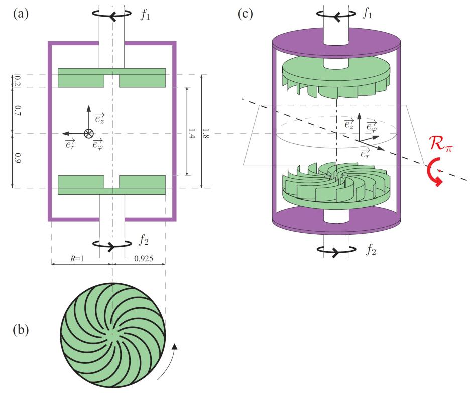
Our experimental setup consists of a Plexiglas cylinder of radius $R=100$ mm filled up with either water or water-glycerol mixtures (cf. figure 1(a)). The fluid is mechanically stirred by a pair of coaxial impellers rotating in opposite sense. The impellers are flat disks of radius $0.925\,R$, fitted with 16 radial blades of height $0.2\,R$ and curvature radius $0.4625\,R$ (cf. figure 1(b)). The disks inner surfaces are $1.8\,R$ apart setting the axial distance between impellers from blades to blades to $1.4\,R$. The impellers rotate, with the convex face of the blades pushing the fluid forward, driven by two independent brushless 1.8 kW motors. The rotation frequencies $f_{1}$ and $f_{2}$ can be varied independently from $1$ to $12$ Hz, speed servo loop control ensuring a precision of $2\permil$ for the mean frequency $f=(f_{1}+f_{2})/2$ and, for the relative frequency difference $\theta=(f_{1}-f_{2})/(f_{1}+f_{2})$, an absolute precision of $1\times 10^{-3}$ and a stability along time better than $0.5\times 10^{-3}$.

Velocity measurements are performed with a SPIV system provided by DANTEC Dynamics. The cylinder is mounted inside a water or glycerol filled square Plexiglas container in order to reduce optical deformations. Two digital cameras are aiming at a meridian plane of the flow through two perpendicular faces of the square container providing 2D-maps of the three-components velocity field. Correlation calculations are performed on $32\times 32$ pixels² windows with $50\%$ overlap. As a result, each velocity is averaged on a $4.16\times 4.16$ mm² window over the $1.5$ mm laser sheet thickness. The spatial resolution is $2.08$ mm. The data provide the radial $u_{r}$, axial $u_{z}$ and azimuthal $u_{\varphi}$ velocity components on a 95$\times$66 points grid through time series of $400$ to $27\,000$ fields regularly sampled, at frequencies from 1 to 15 Hz, depending on the turbulence intensity and the related need for statistics.

The control parameters of the studied von Kármán flow are:

1. the Reynolds number $Re=2\pi fR^{2}/\nu$, where $\nu$ is the fluid viscosity, which controls the intensity of turbulence and,

2. the rotation number $\theta=(f_{1}-f_{2})/(f_{1}+f_{2})$, which controls the asymmetry of the forcing conditions.

     

Figure 1: Schematic view of (a) the experimental setup and (b) the impellers blade profile. The arrow indicates the rotation sense. (c) 3D-view and symmetry : the system is symmetric with respect to any $\cal{R}_{\pi}$-rotation of angle $\pi$ around any line in the equatorial plane which crosses the rotation axis.

2.2 System symmetry vs. flow symmetry

With exact counter-rotation of the impellers, i.e. when $\theta=0$, the experimental system (cf. figure 1(a)) is symmetric with respect to any $\cal{R}_{\pi}$-rotation exchanging the two impellers: the problem conditions are invariant under $\pi$-rotation around any radial axis passing through the center of the cylinder (cf. figure 1(c)). The symmetry group for such experimental system is $O(2)$ [22]. When the motors frequencies differ, i.e. when $\theta\neq 0$, the experimental system is no longer $\cal{R}_{\pi}$-symmetric and the symmetry switches to the $SO(2)$ group of rotations. However, the parameter $\theta$, when small but non-zero, can be considered as a measure of the distance to the exact $O(2)$ symmetry: the stricto sensu $SO(2)$ system at small $\theta$ can be considered as a slightly broken $O(2)$ system. Such perturbative approach of the symmetry breaking has been successfully applied [23, 24] for the 1:2 spatial resonance (or $k-2k$ interaction mechanism) with slightly broken reflection symmetry.

Driven at a given $\theta$ and a given $Re$, the system produces a flow. This flow —or at least its time-average at high $Re$— may be —or may not be— $\cal{R}_{\pi}$-symmetric. The problem is now to define a scalar quantity $S$, equivalent to an order parameter, which can quantify the distance of the flow to the $\cal{R}_{\pi}$-symmetry. The evolution of $S$ with $\theta$ will measure the response of the flow to the symmetry of the forcing and $\chi=\partial S/\partial\theta$ will measure the corresponding susceptibility. Identification of relevant $S$ can be made by studying the flow topology in the laminar and steady regime, at low Reynolds number, i.e. for $Re\lesssim 200$.

2.3 The von Kármán flow topology: the laminar case

Figure 2: Maps of velocity fields in the meridian plane $(r,z)$ —the rotation axis is vertical at $r=0$ and the $r\leftrightarrow-r$ symmetry of the maps reveals the flow axisymmetry— for the laminar ($Re=120\pm 25$) von Kármán flow for different values of the symmetry control parameter $\theta$: (a) $\theta=0$, (b) $\theta=-0.11$, (c) $\theta=-0.19$, (d) $\theta=-1$. The color maps, from blue to red (“jet” colormap), the azimuthal velocity $u_{\varphi}$, whereas the arrows map the $(u_{r},u_{z})$ field. The resolution of the fields has been reduced by a factor 2 for better visibility. Positions $r$ and $z$ are given in units of vessel radius $R$.

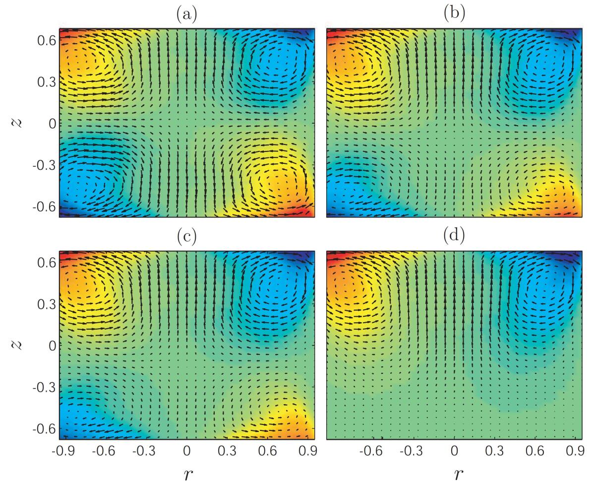
When $\theta=0$, the produced laminar flow is steady and composed of two toric recirculation cells separated by an azimuthal shear layer located at $z=0$ (cf. figure 2(a)) reflecting the $\cal{R}_{\pi}$-symmetry of the system. Actually, each impeller pumps the fluid located near the rotation axis into its center before expelling it radially. This centrifugal pumping creates a toric recirculation cell in front of each impeller. In parallel, in each of the two toric cells, the fluid is rotating in the azimuthal direction following the nearest impeller. Then, when the motors frequencies differ, i.e. when $\theta\neq 0$, the shear layer moves towards the slowest impeller, breaking the symmetry of the flow, but keeping the two-cells topology (cf. figures 2(b-d)). As $\theta$ tends to $\pm 1$, the flow continuously tends to a one-cell topology i.e. a topology with a single toric recirculation cell.

2.4 Identification of two order parameters and associated susceptibilities

We will use two different order parameters to quantify the distance of the flow to the $\cal{R}_{\pi}$-symmetry. First, we consider a local quantity: the $z$-position of the shear layer of the flow, i.e. the position $z_{s}$ of the stagnation point on the rotation axis. The stagnation point position $z_{s}$ is only defined when the flow has the particular two-recirculation-cells axisymmetric structure and will not be suitable —because non-defined— to monitor the distance of the instantaneous flow to the $\cal{R}_{\pi}$-symmetry when it is turbulent. For this purpose, we prefer a second order parameter, a global quantity, the normalized and space-averaged angular momentum $I(Re,\theta,t)$ :

$$I(t)=\frac{1}{\cal{V}}\int_{\cal{V}}rdrd\varphi dz\,\frac{ru_{\varphi}(t)}{\pi\,R^{2}\,(f_{1}+f_{2})}$$ (1)

where $\cal{V}$ is the volume of the flow. Practically, $I(t)$ is computed from SPIV-data restricted to a meridian plane only but, since azimuthal flow fluctuations are strong, time-average over several impeller rotation periods —statistically equivalent to spatial azimuthal averaging— estimate correctly the 3D-value of $I(t)$ (see details in reference [25]).

Figure 3: Global angular momentum $I(t)$ as a function of non-dimensional time $f.t$ for experiments performed at $Re=126\,700\pm 200$ with (a) $\theta=0\pm 10^{-4}$ and (b) $\theta=-0.0084$ and (c) at $Re=890\,000$ and $\theta=0$. Green thin signals are SPIV data $I(t)$ sampled at 15 Hz and blue thick signals correspond to low-pass filtered data $I_{f}(t)$. Corresponding right figures shows the probability density functions (PDF) of the signals with same color code. The red lines indicate the most-probable values of $I_{f}(t)$.

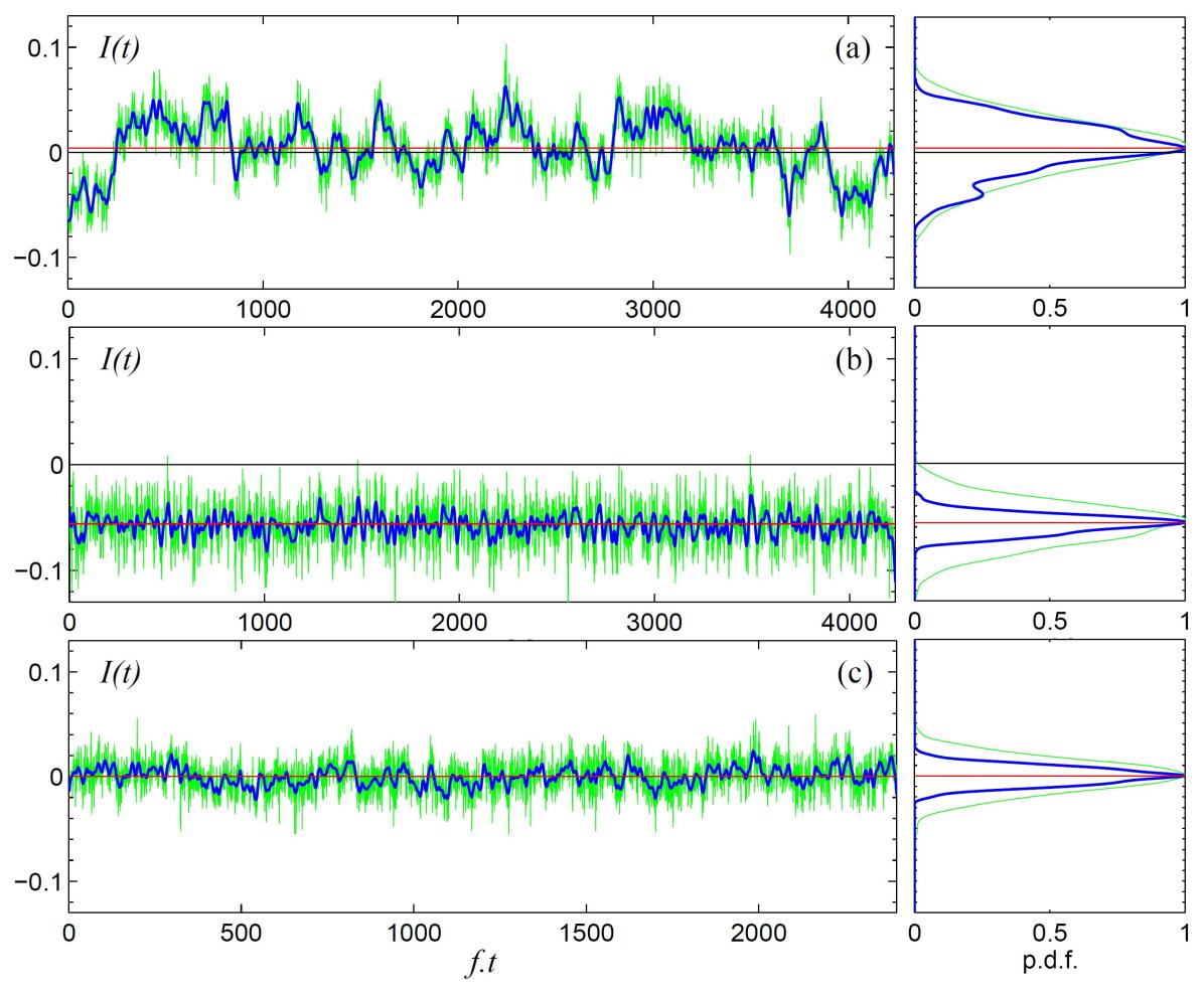
Examples of time-series of $I(t)$ in turbulent regimes are provided below in figure 3 and reveal that strong spontaneous symmetry fluctuations can occur (cf. figure 3(a) for $Re=126\,000$, $\theta=0$). We assume that ergodicity holds, meaning that the instantaneous turbulent flow is exploring along time its energy landscape according to its statistical probability. In this framework, the time average value $\overline{I}$ of $I(t)$ is equivalent to a statistical mechanics ensemble average providing the average is performed over a long enough duration —comparable to the averaging time needed to measure $z_{s}$— in order to correctly sample the slowest time-scales. The quantity $I$ shows the major advantage of being, contrary to $z_{s}$, a robust observable since it is defined for each instantaneous velocity field whatever the structure of the flow and therefore even for turbulent flows. When observing the statistics of the fluctuations of $I$, we will sometimes encounter non-Gaussian and even multi-peaked distributions. Therefore, we will consider the time average $\overline{I}$, the most probable value(s) $I_{*}$ and the fluctuations $I(t)$ of the global angular momentum $I$ to characterize the mean, most-probable and instantaneous symmetry of the flow.

Then, using order parameter $I$, we define two susceptibilities of the flow to symmetry breaking $\chi_{I}$ and $\tilde{\chi}_{I}$, based respectively on the mean and most-probable values of $I$, as:

$$\chi_{I}=\left.\frac{\partial\overline{I}}{\partial\theta}\right|_{\theta=0}\;\;\;\rm{and}\;\;\;\tilde{\chi_{I}}=\left.\frac{\partial{I_{*}}}{\partial\theta}\right|_{\theta=0}.$$ (2)

Another susceptibility may also be defined using $z_{s}$ as:

$$\chi_{z}=\left.\frac{dz_{s}}{d\theta}\right|_{\theta=0}.$$ (3)

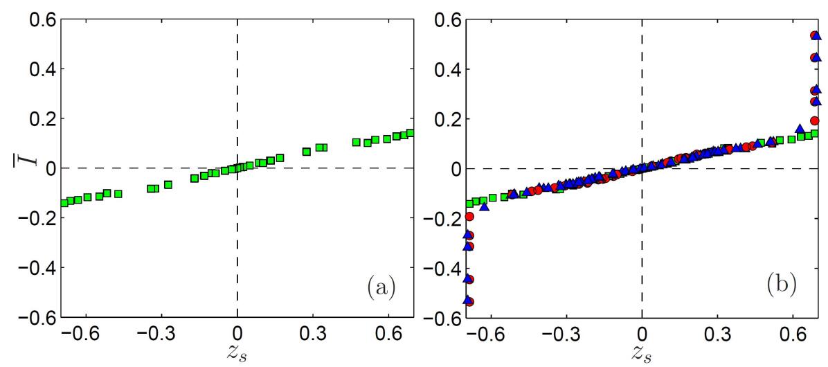
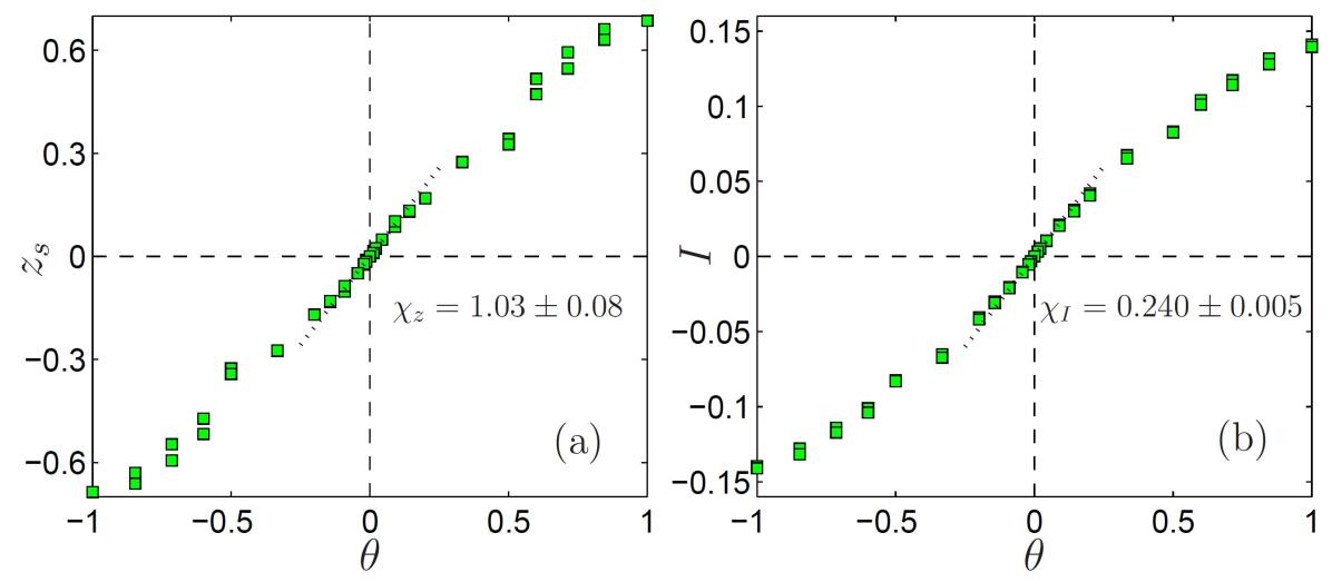
Finally, since our observations (cf. figure 4) have shown that $\overline{I}$ is strictly proportional to the mean altitude $z_{s}$ of the shear layer, with $\overline{I}/z_{s}=0.23\pm 0.01$ whatever $Re$, we may simply use the susceptibilities $\chi=\chi_{I}=0.23\chi_{z}$ and $\tilde{\chi}=\tilde{\chi}_{I}$. In the sequel, we investigate the influence of turbulence on these order parameters —$z_{s}$ and $I(t)$— and the associated susceptibilities as $Re$, and therefore turbulence intensity, increases from $10^{2}$ to $10^{6}$.

Figure 4: Experimental observation of proportionality between time-averaged global angular momentum $\overline{I}$ and mean shear layer altitude $z_{s}$ for (a) laminar flow $Re=120\pm 25$ (green squares, $\overline{I}/z_{s}=0.235\pm 0.005$) and (b) turbulent flows at $Re=67\,000$ (red circles, $\overline{I}/z_{s}=0.227\pm 0.005$) and $Re=890\,000$ (blue triangles, $\overline{I}/z_{s}=0.23\pm 0.01$). Each data series is obtained through plotting $\overline{I}(\theta,Re)$ as a function of $z_{s}(\theta,Re)$ for varying $\theta$ and constant $Re$. At high $Re$, this proportionality holds for $-0.1\lesssim\theta\lesssim 0.1$, i.e. while the shear layer position $z_{s}$ is not saturated to the impellers positions $\pm 0.7\,R$.

2.5 About the statistics of the time-series and high-frequency noise

The statistics of the long time series of $I(t)$ obtained from SPIV data represent a crucial step in our study but they are limited by storage space and computing time. Our results are partly based on the mean values $\overline{I}$ and its equivalent $z_{s}$ computed on mean velocity fields and these lowest moments are well converged for all the data presented. Since statistical physics generally considers the most probable value of a distribution rather than its mean value and since some signals appear multivalued (cf. figure 3(a) and figure 8 below), we are also interested in measuring absolute and relative most-probable values. However, the PDFs of the all raw signals $I(t)$ are almost Gaussian and symmetric. Low-pass-filtering applied on $I(t)$ with a typical $0.15$Hz-cutoff removes some high-frequency noise, due in particular to the small scales of turbulence, and leads to PDFs with relevant non-Gaussian shapes. The best example is the high-resolution time-series corresponding to the highest fluctuation-level measured at $Re=39\,000$, presented in figure 8. The most-probable values are computed accordingly, but because of statistical limitations, these value are less converged than mean values.

2.6 Formal analogy with ferromagnetic systems

In the non-fluctuating laminar case, when $\theta=0$, $\overline{I}$ is strictly equal to zero due to the symmetry of the flow. In contrast, as $\theta$ drifts away from $0$, the value of the angular momentum $\overline{I}$ becomes more and more remote from zero as the asymmetry of the flow grows. In the turbulent regimes, the same behavior is observed but with higher susceptibilities to symmetry breaking, i.e. higher sensitivity to $\theta$.

In such a framework, the Reynolds number —or a function of it [26]— is the equivalent of a statistical temperature and we are entitled to propose the following formal analogy between ferromagnetic systems and von Kármán systems:

• Order parameter: magnetization $M$ $\Leftrightarrow$ angular momentum $I$;

• Symmetry breaking parameter: external applied field $h$ $\Leftrightarrow$ relative driving asymmetry $\theta$;

• Control parameter: temperature $T$ $\Leftrightarrow$ Reynolds number $Re$, or a function of it.

3 Laminar and turbulent flow: influence of $\theta$ and $Re$

Figure 5: (a) axial position $z_{s}$ of the stagnation point and (b) global angular momentum $I=\overline{I}$ as a function of $\theta$ for the laminar flows at $Re=120\pm 25$.

3.1 The laminar susceptibility

The evolutions of the symmetry parameters $z_{s}$ and $\overline{I}$ as a function of $\theta$ in the laminar flow at $Re=120\pm 25$ are provided in figure 5. In this case $\overline{I(t)}=I(t)$ and $z_{s}$ are defined for each instantaneous field. We see that $z_{s}$ evolves almost linearly with $\theta$ from $z_{s}=-0.7\,R$ (position of impeller 1) for $\theta=-1$ to $z_{s}=0.7\,R$ (position of impeller 2) for $\theta=1$, through $z_{s}=0$ for $\theta=0$ (cf. figure 5(a)). Variation of $I$ with $\theta$ is similar. In the central region, the linearity is excellent and we measure $\chi_{z}=1.03\pm 0.08$ and $\chi_{I}=0.240\pm 0.005$.

3.2 Flow topology : the turbulent case

Figure 6: Maps of mean velocity fields of the turbulent von Kármán flow at $Re=890\,000$ for different values of $\theta$: (a) $\theta=0$, (b) $\theta=-0.0036$, (c) $\theta=-0.0147$, (d) $\theta=-1$, with same layout as figure 2. The $r\leftrightarrow-r$ symmetry of the maps reveals that the time-averaged mean fields are axisymmetric.

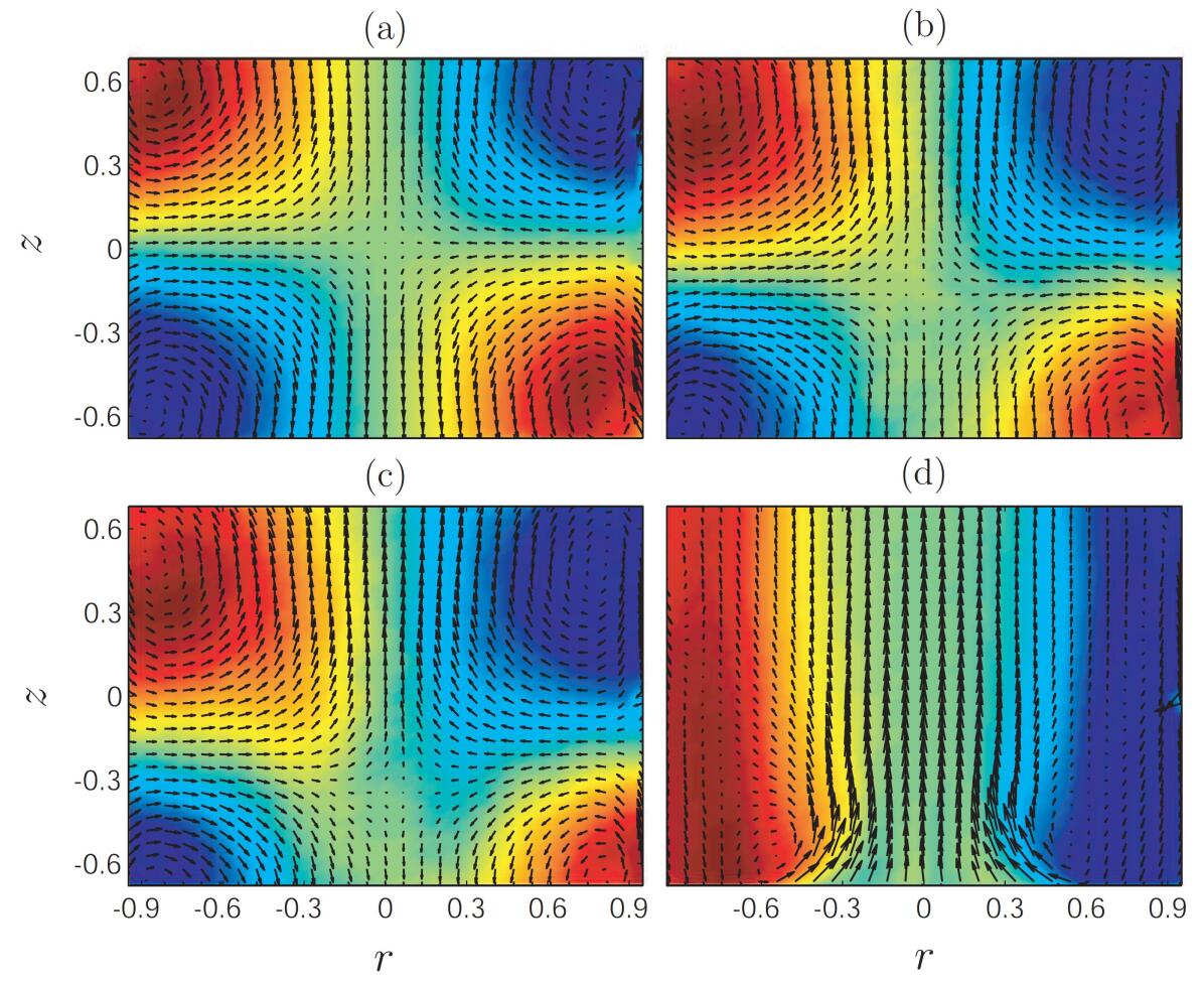
Increasing the Reynolds number, one expects to reach fully developed turbulence around $Re=10\,000$ [11]. In this turbulent regime and at $\theta=0$, the $\cal{R}_{\pi}$-symmetry is broken for the instantaneous flow. However, as usually observed for classical turbulence, this symmetry is restored for the time-averaged flow (cf. figure 6(a)). Then, as in the case of the laminar flow, when $\theta$ is varied, we observe the breaking of the $\cal{R}_{\pi}$-symmetry of the turbulent mean flow, the structure of which matches quite well the laminar flow topologies, however with a higher sensitivity to $\theta$ (cf. figures 6(b-d)).

3.3 The turbulent susceptibility

Figure 7: Turbulent regimes at $Re=67\,000\pm 2\,000$ (red circles) and $Re=890\,000\pm 140\,000$ (blue triangles): axial position of the stagnation point $z_{s}$ (a-b) and global angular momentum $I$ —mean $\overline{I(t)}$ (c-d) and standard error $\sigma_{I}$ (e-f)— as a function of $\theta$. Wide span $-0.3<\theta<0.3$ on the left side (a,c,e) and $\times 10$ zoom $-0.03<\theta<0.03$ on the right side (b,d,f). Data for the laminar regime at $Re=120$ (green squares) from figure 5 are also plotted for comparison. The data have been symmetrized with respect to $\theta=0$. Dashed lines in (d) indicates the tilted plateaus independent of $Re$ and their extrapolations to $\pm I_{0}$.

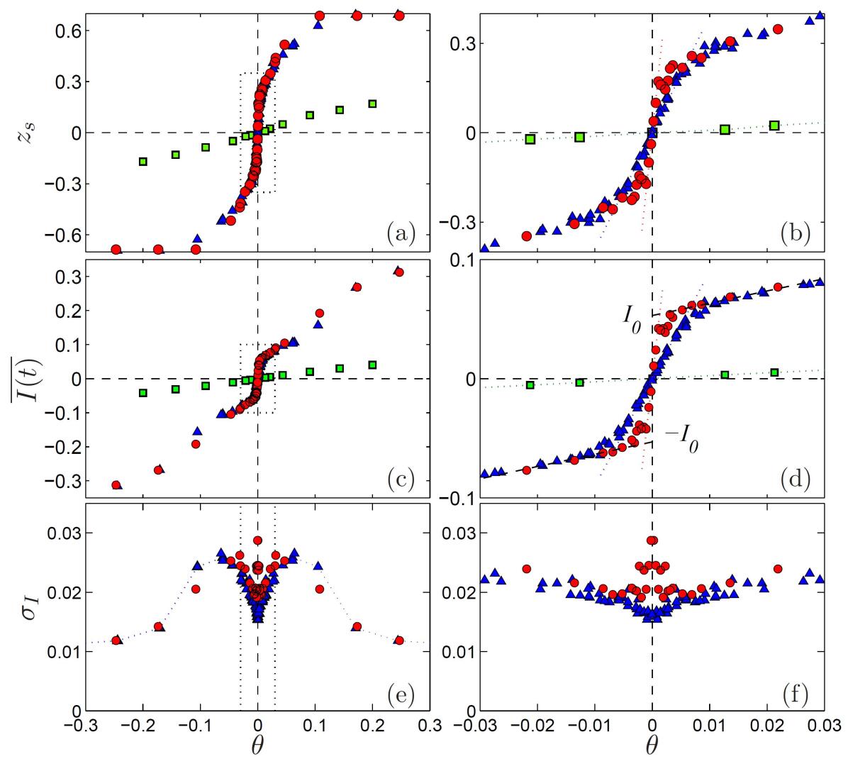
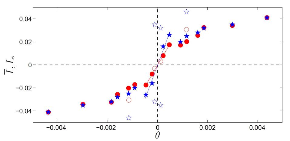
The main properties of $z_{s}$ and $I$ with respect to $\theta$ can be observed in figure 7 which combines the measurements obtained at an intermediate Reynolds number $Re=67\,000\pm 2\,000$ (red circles) as well as at the highest reachable Reynolds number in our experiment $Re=890\,000\pm 140\,000$ (blue triangles). The left-hand-side figures give a global view over a large span in $\theta$: at this scale the two high-Reynolds-number series appear very close to each other and show much higher susceptibilities than the laminar flow series (green squares): turbulence enhances dramatically the sensitivity of the flow to symmetry breaking. The turbulent susceptibilities are at least 10 times larger than the laminar susceptibility since $z_{s}$ saturates —the shear layer disappears into one impeller— for $|\theta|$ larger than a finite and small value $\theta_{c}=0.10\pm 0.02$, close to the value predicted in [27] for flat disks and 10 times smaller than in the laminar case where the shear layer disappears asymptotically as $\theta\rightarrow\pm 1$ (cf. figure 2 and 5(a)). These disappearances of the shear layer into impeller 1 or impeller 2 correspond to the transitions of the flow topology from two recirculation cells —at small $|\theta|$— to a single recirculation cell —at large $|\theta|$. In figure 7(e), we observe two maxima for $\sigma_{I}$, the level of fluctuations of $I$, around $\pm\theta_{c}$, which are characteristic of these transitions. Such transitions have already been studied for other counterrotating von Kármán flows in subcritical cases [10, 25].

The effect of the Reynolds number on turbulent flow responses is revealed by the $\times 10$-zooms in $\theta$ on the right-hand-side of figure 7. It is clear that, in a narrow region $|\theta|\lesssim 0.01$, we encounter two major differences between the $Re=67\,000$ and $Re=890\,000$ experiments:

• The susceptibilities are very different: $\chi_{I}=42\pm 1$ at $Re=67\,000$ and $\chi_{I}=9\pm 1$ at $Re=890\,000$ (cf. figure 7(b,d)), respectively $175$ and $37$ times the laminar value.

• The fluctuation level $\sigma_{I}(\theta)$ presents a sharp and narrow peak at $\theta=0$ for $Re=67\,000$, but not for $Re=890\,000$ (cf. figure 7(f)).

This peak is typical of all data in the intermediate Reynolds number range $20\,000\lesssim Re\lesssim 200\,000$ where the susceptibility is clearly higher than around the highest Reynolds number reached $Re\sim 10^{6}$. Note that outside the active region of high susceptibility and high fluctuations $|\theta|\lesssim 0.01$, there is no more $Re$-dependency for $\overline{I}(\theta)$: in the medium range $0.01\lesssim|\theta|\lesssim 0.05$, not too close from the two-cells/one-cell transition at $\pm\theta_{c}$, all curves collapse on tilted plateaus which —if extrapolated— cross the $\theta=0$ axis at $I_{0}\simeq\pm 0.05$ whatever $Re$.

3.4 Fluctuation level near $\theta=0$

For all Reynolds numbers in the intermediate range, we observe a sharp and narrow peak for the fluctuation level $\sigma_{I}(\theta)$ around $\theta=0$. This is illustrated by two time-series at $Re=127\,000$, in figure 3(a) and (b), for $\theta\simeq 0$ and $\theta=0.0084$ which correspond respectively to the top and the bottom of the fluctuation peak in figure 7(f). The difference between the two signals is striking and reveals that the fluctuation peak is due to the presence non-Gaussian intermittencies. These intermittencies have been observed in the range $|\theta|\lesssim 5\times 10^{-3}$ exclusively. The $I(t)$ time-series at $Re=890\,000$ and $\theta=0$, in figure 3(c), corresponds however to the minimum fluctuation level of figure 7(f): the corresponding PDF is narrow, symmetric and has a single central maximum.

3.5 Mean vs. most-probable values for highly intermittent regimes

Figure 8: (a) Global angular momentum $I(t)$ for an experiment performed at $Re=39\,000$ for $\theta=\overline{\theta(t)}=0$. The green thin line is SPIV data $I(t)$ sampled at 15 Hz and the blue thick line corresponds to 0.15 Hz low-pass filtered data $I_{f}(t)$. (b) Probability density functions (PDF) with the same color code. Blue dashed lines indicate the two most-probable values $\pm I_{*}$ of $I_{f}(t)$ and green dash-dot lines indicate the mean value $\overline{I}$. (c) Time-series of $\theta(t)$ as produced by the motor regulation in unit of $10^{-3}$: the correlation with $I(t)$ is negligible (see text).

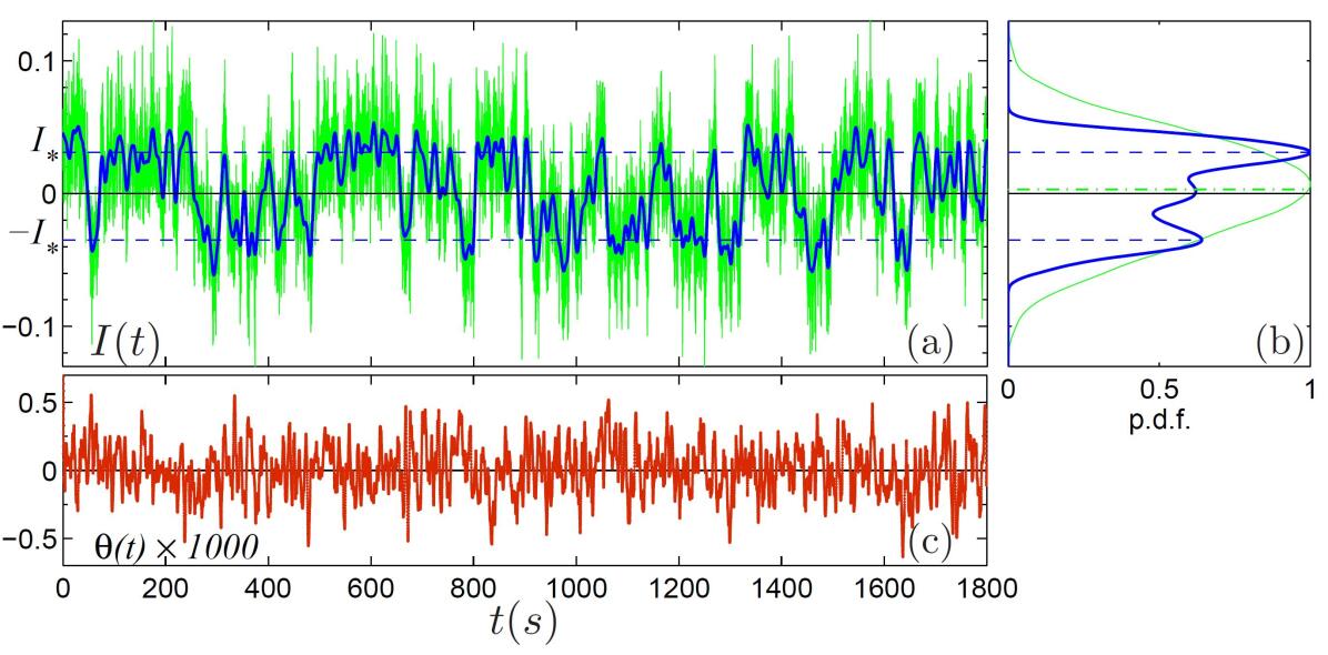
In the above paragraphs and figures we have presented the evolution of mean values of $I(t)$ with $\theta$ for different $Re$. Globally, most-probable values differ from mean values only when the susceptibility is high and are, in absolute value, greater than mean values. This difference is especially noticeable for $Re$ around $40\,000$. The data set which corresponds to the maximum fluctuation level is presented in figure 8 where $\overline{I}\simeq 0$. It shows strong temporal intermittency between states of different angular momentum values revealed by the multi-peak PDF.

The most-probable values of $I(t)$ are plotted in figure 9, with respect to $\theta$ very close to $\theta=0$. We observe that for $Re=37\,000\pm 2\,000$, the slope $\tilde{\chi}$ for most-probable values is approximately twice the slope $\chi$ for mean values at $\theta=0$. We also reported points obtained from three high-resolution time-series at $Re=39\,000$ (figure 8) and $43\,000$. For these data sets, we plot the first two most-probable values $\pm I_{*}$ of $I(t)$ corresponding to the two almost symmetric peaks of the PDFs with are exchanging their relative importance around $\theta=0$. These values are significantly higher than those of the $Re=37\,000$-data series. This can be due to either the proximity of the critical value $Re_{c}$ or to the limited statistics of the $Re=37\,000$-data series. Anyhow, these results suggest that the corresponding susceptibility $\tilde{\chi}$ is diverging at $Re=41\,000\pm 2\,000$ as it will be discussed in the next section.

Figure 9: Mean $\overline{I}$ (red circles) and most-probable $I_{*}$ (blue stars) values of the global angular momentum $I(t)$ for $Re\sim 40\,000$. Close symbols come from a set of moderate-resolution data at $Re=37\,000\pm 2\,000$ ($f=12$Hz, $1\,200$ SPIV fields acquired at $1.7$Hz), whereas open symbols come from high-resolution time-series at $Re=41\,000\pm 2\,000$ ($f=8$Hz, $9\,000$ or $27\,000$ SPIV fields acquired at $15$Hz as, e.g., in figure 8) acquired in a different glycerol-water mixture. The data have been symmetrized with respect to $\theta=0$ and, for the data point at $\theta\simeq 0$ of the second series, we plot the two most-probable values $\sim\pm I_{*}$ corresponding to the two peaks of the PDFs as in figure 8(b).

3.6 Divergence of the susceptibility at $Re\simeq 40\,000$

From the above results it is clear that the effect of the Reynolds number is to be studied for $\theta=0$. The present section deals with the susceptibilities and the fluctuation level at $\theta=0$ and for $Re$ covering the whole study range $10^{2}-10^{6}$.

Figure 10: Reynolds number dependence of the symmetry-breaking susceptibility of the von Kármán flow at $\theta=0$ (a) and its inverse (b). Black open symbols correspond to susceptibility $\chi=\chi_{I}=0.23\chi_{z}$ obtained from mean values $\overline{I}$ (squares) and $z_{s}$ (diamond); red full circles stands for $\tilde{\chi}_{I}$ obtained from most-probable values $I_{*}$ of $I$. The red full star corresponds to the region ($Re=41000\pm 2000$) where infinite susceptibility is inferred from the strong multistability of the signal (cf. figures 8 and 9). Dashed lines are fits of the most-probables values above and below the star as linear functions of $1/\log(Re)$ as proposed in the discussion of section 6.2. (c) Standard deviation $\sigma_{I}$ of the unfiltered global angular momentum $I(t)$ at $\theta=0$.

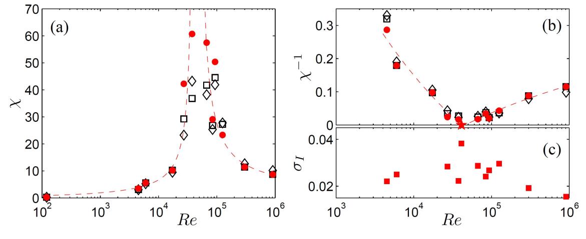
In figure 10(a), we plot susceptibility measurements —$\chi$ and $\tilde{\chi}$, cf. equation 2— as a function of $Re$. Figure 10(b) shows the inverses of these values and figure 10(c) the corresponding standard deviation $\sigma_{I}$ of $I(t)$. The susceptibility $\tilde{\chi}$ based on the most probable values $I_{*}$ of $I(t)$ and the fluctuations of $I(t)$ are both maximum for $Re\simeq 40\,000$. However, as reported earlier [21], the susceptibility $\chi$ based on the mean values of $I(t)$ reaches a maximum for higher $Re\simeq 90\,000$. We also note that $\tilde{\chi}\apprge\chi$, whatever $Re$, and that the highest measured susceptibilities are of the order of the highest measurable values considering the $\theta$-precision of our setup.

All the above results suggest a divergence of $\tilde{\chi}(Re)$ which clearly appears with the fits in figures 10(a) and (b): $\tilde{\chi}(Re)$ diverges at $Re=Re_{c}=40\,000\pm 5\,000$ with critical exponent $-1$ [illustrated in figure 10 with respect to $1/\log(Re)$ (see discussion in section 6.2)] and resembles a classical magnetic susceptibility divergence at the ferromagnetic/paramagnetic phase transition. In the next section, we investigate further this transition by looking at the equivalent of the spontaneous magnetization of magnets, i.e. how, around $Re_{c}$, the angular momentum $I(t)$ spontaneously and dynamically transits between different finite values.

4 Dynamic multistability near $Re_{c}$ and spontaneous “momentization”

4.1 Observation of the dynamics at $Re=39\,000$

Close to the susceptibility divergence, we observe a complex dynamics for the global angular momentum $I(t)$, as illustrated in figure 8 at $Re=39\,000$ and $\theta=0$. Indeed, one observes that $I(t)$ does not just fluctuate randomly around zero —its mean value— but shows a tendency to lock for some times, preferentially around $\pm I_{*}$ with $I_{*}$ of the order of $0.03$-$0.04$, estimated from the main peaks of the PDF of the filtered signal $I_{f}(t)$ (cf. figure 8(b)).

In order to understand the nature of the fluctuations of $I(t)$, we have first checked that $I(t)$ is uncorrelated with the control parameter $\theta(t)$ (correlation coefficient $C(I,\theta)=\overline{I(t)\,\theta(t)}/\sigma_{I}\,\sigma_{\theta}<0.02$, cf. figures 8(a,c)) and thus reveals only spontaneous fluctuations. Actually, $I(t)$ fluctuates with two separate time scales: (i) fast fluctuations related to “traditional” small-scale turbulence and (ii) intermittencies corresponding to residence time of typically few tens of seconds and certainly due to the proximity of the susceptibility divergence. If one performs a time-average of the velocity field over one of these intermittent periods, one obtains a time localized “mean” flow, analogous to what is obtained for true mean flows when $\theta\neq 0$ as presented in figures 6(b-c), and with its own level of spontaneous symmetry breaking. To go one step further with the correspondence between $I(t)$ and the amount of symmetry breaking or the position of the shear layer, we have computed bin-averages of the velocity field for a time-series $I(t)$ in 11 bins ranging from $-0.075$ to $+0.075$. In figures 11(a-c), we have plotted three examples of such bin-averaged fields. The pattern is $\cal{R}_{\pi}$-symmetric for the bin around zero (cf. figure 11(b)) and non-symmetric otherwise (cf. figures 11(a) and (c)). From the resulting series of conditionally-averaged velocity fields we measure the stagnation point axial position $z_{s}$ and report it as a function of the mean bin value (cf. figure 11(d)). There is a very good matching between these bin-averaged data and the time-averaged data already presented in figure 4 for different $\theta$: beyond the proportionality between $z_{s}$ and $\overline{I}$, $I(t)$ can thus definitively be used as a quantitative instantaneous symmetry measurement. For example, the two symmetrical most-probable values $\pm I_{*}$ of $I(t)$ correspond typically to $|z_{s}|\simeq 0.2\,R$.

Figure 11: Bin-averaging of the velocity field with respect to $I(t)$ for $Re=39\,000$ and $\theta=0$ (same data series as in figure 8). Three bin-averaged velocity fields are presented for bins: (a) $-0.075<I_{f}(t)<-0.050$, (b) $-0.0125<I_{f}(t)<0.0125$ and (c) $0.0375<I_{f}(t)<0.0625$. (d) Corresponding stagnation point axial position $z_{s}$ measured for 11 such bin-averaged fields for $I$ between $-0.075$ and $+0.075$ (green stars), superimposed to regular time-averaged data for varying $\theta$ at $Re=67\,000$ (red circles) and $Re=890\,000$ (blue triangles) as in figure 4(b).

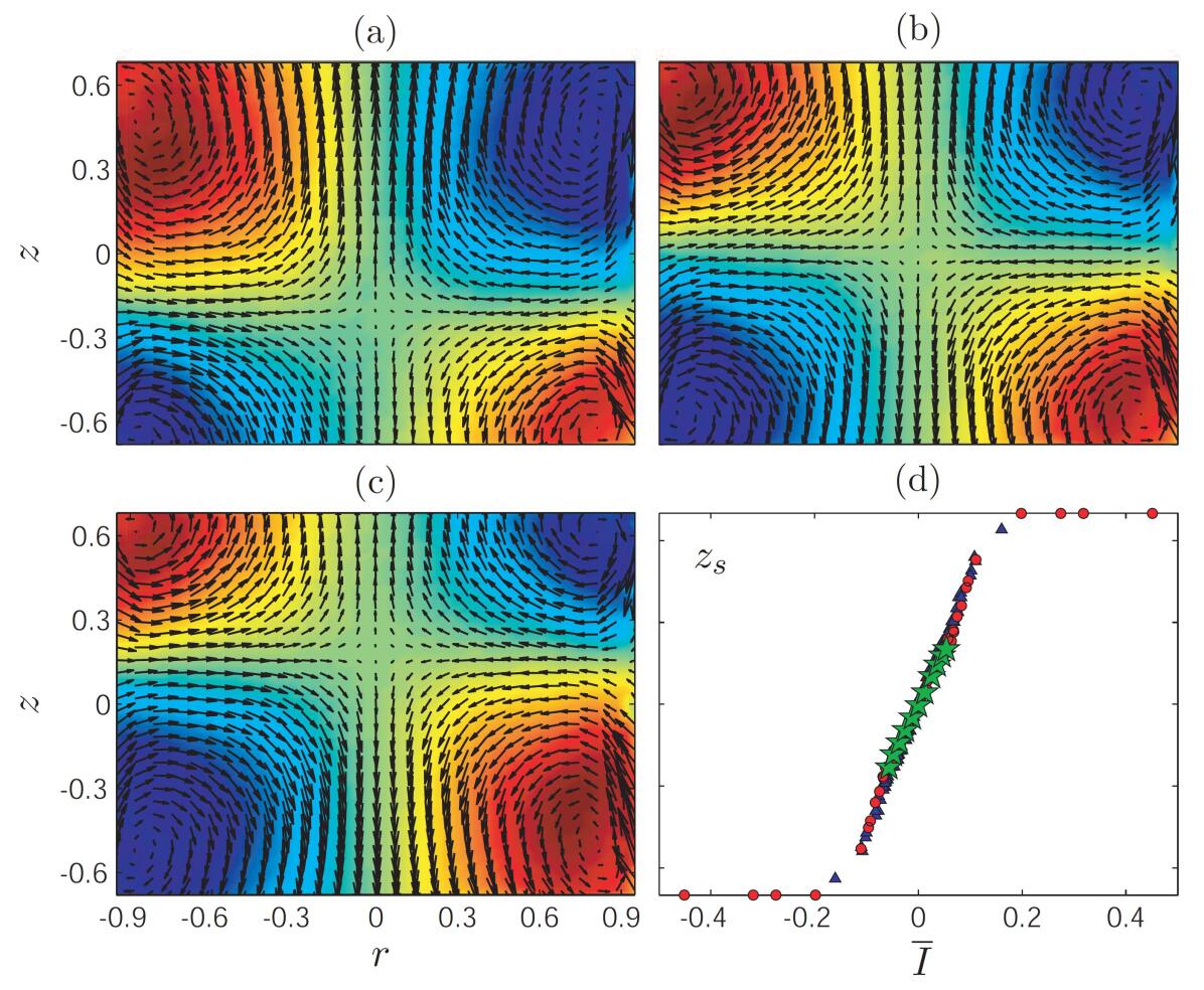
From the above observations, we can conclude that, very close to $Re_{c}$, the turbulent flow explores a band of metastable symmetry breaking patterns evidenced by $-I_{*}\lesssim I_{f}(t)\lesssim+I_{*}$, where $I_{f}(t)$ is the $0.15$Hz low-pass filtered value of $I(t)$, the three most-visited states being $-I_{*}$, $0$, and $+I_{*}$. Farther from $Re_{c}$, signals and PDFs also reveal coexisting preferred values for $I(t)$ when $\theta$ is very small.

4.2 The “momentization”

The dynamical spontaneous symmetry breaking observed in our experiment can be seen as the coexistence of multistable/metastable steady states of different symmetry which are explored dynamically along time. By analogy with magnetization we propose to describe this as successive “momentization” patterns observed in time, thanks to ergodicity which arises from the very high level of fluctuations.

With respect to magnetism, the main difference is that the spontaneous momentization occurs along time and mainly very close to the critical point. Furthermore, owing to the statistical limitations, we cannot conclude if momentization occurs only on one side of the transition —as it is for the ferro/para transition— or on both sides.

4.3 Statistics of the dynamic multistability

The metastable/multistable states of finite lifetime ($\tau$) observed in time-series such as in figure 8(a) can be characterized by their angular momentum averaged over their lifetime and noted $\overline{I}^{\tau}$, to avoid confusion with the full-signal mean value $\overline{I}$. The $\overline{I}^{\tau}$ are distributed along the angular momentum axis and we note ${\cal{I}}(Re,\theta)$ the $I$-interval containing the distribution for experiments at $(Re,\theta)$.

Multistability is systematically observed in the high susceptibility zone limited by $Re\in{\cal{I}}_{Re}\sim[20\,000,200\,000]$ and $\theta\in{\cal{I}}_{\theta}\sim[-0.01,+0.01]$. Whatever $Re$ and $\theta$ in ${\cal{I}}_{Re}$ and ${\cal{I}}_{\theta}$, we observe that ${\cal{I}}(Re,\theta)$ is confined in $[-I_{0},+I_{0}]$ ($I_{0}$ has been defined at the end of section 3.3 and is shown in figure 7). When $Re\simeq Re_{c}$, the interval ${\cal{I}}(Re,\theta)\simeq[-I_{*},+I_{*}]$ is symmetric and close to $[-I_{0},+I_{0}]$ (cf. figure 8): the whole band is almost populated. However, farther from $Re_{c}$, the interval ${\cal{I}}(Re,\theta)$ is smaller and evolves inside $[-I_{0},+I_{0}]$ with $\theta$.

5 Complementary investigation about the azimuthal structure of the flow

Before discussing our results in the next section, it is important to note that all the above results concern 2D-velocity-fields in a meridian plane: the azimuthal spatial structure is ignored by our 2D-SPIV process since the azimuthal patterns —moving and fluctuating— are averaged along time and not resolved in space at all. In this section, we investigate some preliminary experimental results about the 3D-structure of the flow, gathered by visual observation with bubble seeding and white light [11, 25]. With a high density of bubbles we mostly see the patterns on the outer cylinder which are the radial vortices due to the shear-layer destabilization. In practice, we experience that, even in the flow is turbulent, the azimuthal number $m$ of vortices can be a well defined integer over some ranges of Reynolds number and/or some periods of time. So, exactly as for small dynamical systems, changes in $m$ can reveal an Eckhaus instability for the 3D-mean pattern .

This dynamics has been observed for $22\,000\apprle Re\apprle 300\,000$. Despite the vortices are strongly fluctuating, we can report the following observations of the average number $m$ of vortices around the perimeter of the shear layer at $\theta=0$:

• $m=3$ for $22\,000\apprle Re\apprle 47\,000$,

• $m=4$ for $86\,000\apprle Re\apprle 300\,000$.

Between these two regions, the fluctuations are generally too strong to draw precise conclusions, but at least a clear observation of $m=4$ has been made once at $Re\simeq 51\,000$. So, we conclude that some kind of $m=3\leftrightarrow m=4$ Eckhaus transition occurs between $Re=47\,000\sim Re_{c}$ and $Re=86\,000\sim 2Re_{c}$, in the region of very high susceptibility.

6 Discussion

We have reported the experimental study, for a von Kármán swirling flow, of (i) the response of the mean flow to a continuous breaking of the $\cal{R}_{\pi}$-symmetry of the system and (ii) the spontaneous symmetry fluctuations of the instantaneous flow, from the laminar regime at $Re\sim 10^{2}$ to the highly turbulent regime at $Re\sim 10^{6}$. The divergence of the susceptibility $\tilde{\chi}(Re)$ for $Re=Re_{c}=40\,000\pm 5\,000$ reveals the existence of a phase transition or a bifurcation. In the following, we discuss the implications of this phase transition for turbulence, the critical behaviors and the analogy with the para-ferromagnetic transition.

6.1 A Reynolds-dependent turbulence

This new transition makes some non-dimensional characteristic quantities of the flow still $Re$-dependent at very high $Re$. The turbulence is thus definitively not fully developed in this closed turbulent flow, contrary to the most common observations in this Reynolds number range. In other closed flows, the literature reports some examples of transitions occurring at Reynolds number of the order of $10^{5}$, a decade in $Re$ beyond where the turbulence already looks like fully developed. First, in various type of turbulent fluid experiments, several authors report transitions and symmetry breaking at high Reynolds number (cf., e.g., references [4, 5, 6, 7]). Moreover, in a similar von Kármán flow, de la Torre and Burguete [12, 13] observed a bistability between two broken $O(2)$-symmetry states with $z_{s}/R=\pm 0.19$. Although the slow dynamics is very different from what is reported here, both experiment are likely to belong to a common framework (see below). Finally, in a liquid helium von Kármán flow, Tabeling et al. report a local peak in the flatness of velocity derivative around $R_{\lambda}=700$ —corresponding to $Re=2\times 10^{5}$ [8]. An interpretation in terms of a second-order phase transition was proposed [9]. Velocity derivatives cannot be measured in our experiment because of the low spatial resolution of our SPIV system. However, if one could establish that the observations of Tabeling et al. are indeed connected with ours, then our work would prove that their transition is related to the global structure of the mean flow and thus does not result from the breakdown of small-scale vortical structures as proposed in reference [9].

6.2 Critical behaviors and analogy with magnetism

6.2.1 The control parameter: a function of $\log Re$ —

Since our study covers 4 orders of magnitude in Reynolds number, it is natural to acquire and plot results along a logarithmic scale. However, we could search for critical behaviors with either $Re$ or $\log Re$ as control parameter. Indeed, critical behaviors are asymptotic behaviors around a given threshold $Re_{c}$ and therefore both $(Re-Re_{c})$ and $(\log Re-\log Re_{c})$ are mathematically equivalent. However, it is very common in non-linear physics, that asymptotic behaviors or normal forms correctly describe the dynamics, not only asymptotically, but over finite —and even large— ranges around thresholds using one particular control parameter. This is exactly what happens here and because of the quality of the $1/\tilde{\chi}(Re)$ fit in figure 10(b), we conclude that a relevant control parameter for this critical phenomenon can be $\log Re$ or a gentle function of it.

Within the formal turbulence/magnetism analogy, we actually use Castaing’s proposition [26] for a temperature of turbulent flows which is $T\sim 1/\log Re$.

6.2.2 Critical behavior of the susceptibility —

The divergence appears clearly in figure 10(b) where $1/\tilde{\chi}(Re)$ goes to zero at $Re=Re_{c}=40\,000\pm 5\,000$ in a way that can be fitted with a $-1$ critical exponent by:

$$\tilde{\chi}\propto\left|\frac{1}{\log Re}-\frac{1}{\log Re_{c}}\right|^{-1}$$ (4)

with different prefactors below and above $Re_{c}$. This expression can be interpreted as the combination of the Castaing statistical temperature of turbulence $T\sim 1/\log Re$ with the classical mean-field-theory expression for susceptibility at a critical point:

$$\tilde{\chi}\propto\left|T-T_{c}\right|^{-1},$$

Expression (4) has already been successfully used in reference [21] to describe the “mean” susceptibility $\chi$ computed with mean values —instead of most probable values for $\tilde{\chi}$— of $I(t)$ and with a more limited set of data. As already underlined, this rather fair agreement between mean-field-theory and our turbulent measurements is at first surprising. However, recent theoretical developments suggest that in turbulent von Kármán flow the interactions are long-range like [29, 30] supporting therefore the idea that mean field theory is nearly applicable in our system.

6.3 Momentization vs. magnetization

Within the proposed analogy between our observations and the para-ferromagnetism transition, the equivalence between the magnetization and the momentization is the most questioning aspect. In particular, the shape of the $\overline{I}(\theta)$-curves is more similar to the magnetization response curves of a single magnetic domains than to poly-domains.

For the para-ferromagnetism transition, the magnetization increases with the distance below the critical temperature while here, as stated in section 4.3, the spontaneous momentization is finite, limited in amplitude by $I_{0}$, and decreases with the distance to $Re_{c}$. The system may share some characteristics with reentrant noise-induced phase transition similar to that observed in the annealed Ising model [31, 32]. Our system is definitively of finite size and it is thus coherent that both the level of fluctuation $\sigma_{I}(Re_{c})$ and the band of spontaneous fluctuations for $I(t)$ —which corresponds to a finite excursion of the shear layer position along $z$— remain finite at critical point (figure 10(c)).

In their von Kármán experiment at $\theta=0$ and $Re\simeq 4\times 10^{5}$, de la Torre and Burguete ([12, 13]) also observe multistability of three and only three states with can be interpreted, within our framework, as $\overline{I}^{\tau}=-I_{*}$, $0$ and $+I_{*}$. While the amplitude of the $\overline{I}^{\tau}=0$ mode is constant along time, their system switches between the two $\overline{I}^{\tau}=\pm I_{*}$ modes with a very slow dynamics (hours) and very fast transitions. This dynamics does not seem to depend on $Re$ once $Re\gtrsim 2\times 10^{4}$, the symmetric $\overline{I}^{\tau}=0$ state being dominant below. Within our framework, we could propose that, in this experiment, the susceptibility is infinite whatever $Re$ above $2\times 10^{4}$ (cf. figure 5(a) of reference [12]).

6.4 Specificity of turbulent fluctuations with respect to classical thermal noise

In our turbulent system, the observed time-dynamics seems to be due to the very high level of intrinsic turbulent fluctuations, which are very different from classical thermal fluctuations that pilot the dynamics of magnetic momentums. These turbulent fluctuations are considered as the noise or the statistical temperature origin of our system. In classical close-to-equilibrium thermodynamical systems, thermal fluctuation are generally considered as regular additive noise exactly as for the classical treatment of instabilities in the presence of noise where an external noise —additive or multiplicative— is introduced as a perturbation of a regular system [33]. For turbulent flows in general and for our von Kármán flow in particular, the situation is different: the flow itself is intrinsically highly fluctuating so that fluctuations are of the same order of magnitude than the mean values [25] and cannot be treated as perturbations. So, the specific problem our experiment addresses is the behavior of the instability of an average global quantity such as $I(t)$ in an intrinsically fluctuating or noisy system. This is similar to the problem of the experimental dynamo instability [34, 35] which can only occur in turbulent flows because of the nature of the existing conducting fluids of the Universe. Therefore, non-classical behaviors are likely to be observed for bifurcations or phase-transitions in such highly-turbulent flows and our system represents a unique tool to study these transitions.

References

- [1] Landau L D and Lifchitz E M, 1976 Statisticheskaya Fisika Third edition (Moscow: Nauka)
- [2] Manneville P, 1990 Dissipative Structures and Weak Turbulence (Boston: Academic Press)
- [3] Frisch U, 1995 Turbulence - The Legacy of A N Kolmogorov (Cambridge: Cambridge University Press)
- [4] Chillá F, Rastello M, Chaumat S and Castaing B, 2004 Eur. Phys. J. B 40 223
- [5] Mujica N and Lathrop D P, 2006 J. Fluid. Mech. 551 49
- [6] Gibert M, Pabiou H, Tisserand J-C, Gertjerenken B, Castaing B, and Chillà F, 2009 Phys. Fluids 21 035109
- [7] Weiss S, Stevens R J A M, Zhong J-Q, Clercx H J H, Lohse D and Ahlers G, 2010 Phys. Rev. Lett. 105, 224501
- [8] Tabeling P, Zocchi G, Belin F, Maurer J and Willaime H, 1996 Phys. Rev. E 53 1613
- [9] Tabeling P and Willaime H, 2002 Phys. Rev. E 65 066301
- [10] Ravelet F, Marié L, Chiffaudel A and Daviaud F, 2004 Phys. Rev. Lett. 93 164501
- [11] Ravelet F, Chiffaudel A and Daviaud F, 2008 J. Fluid. Mech. 601 339
- [12] de la Torre A and Burguete J, 2007 Phys. Rev. Lett. 99 054101;
- [13] Burguete J and de la Torre A, 2009 Int J. Bifurcation Chaos 19 2695
- [14] Molenaar D, Clercx H J H and van Heijst G J F, 2004 Physica D 196 329
- [15] Bouchet F and Simmonet E, 2009 Phys. Rev. Lett. 102 094504
- [16] Berhanu M et al., 2007 Europhys. Lett. 77 59001
- [17] Petrelis F and Fauve S, 2008 J. Phys.: Condens. Matter 20 494203
- [18] Ciliberto S, Garnier N, Hernandez S, Lacpatia C, Pinton J-F and Chavarria G R, 2004 Physica A 340 240
- [19] Grenard V, Garnier N B and Naert A, 2008 J. Stat. Mech. L09003
- [20] Monchaux R, Cortet P-P, Chavanis P-H, Chiffaudel A, Daviaud F, Diribarne P and Dubrulle B, 2008 Phys. Rev. Lett. 101 174502
- [21] Cortet P-P, Chiffaudel A, Daviaud F and Dubrulle B, 2010 Phys. Rev. Lett. 105 214501
- [22] Nore C, Tuckerman L S, Daube O and Xin S, 2003 J. Fluid Mech. 477 1
- [23] Chossat P, 1993 Nonlinearity 6 723
- [24] Porter J and Knobloch E, 2005 Physica D 201 318
- [25] Cortet P-P, Diribarne P, Monchaux R, Chiffaudel A, Daviaud F and Dubrulle B, 2009 Phys. Fluids 21 025104
- [26] Castaing B, 1996 J. Phys. II 6 105
- [27] Dijkstra G and van Heijst G J F, 1983 J. Fluid Mech. 128 123
- [28] Prigent A, Dauchot O, 2000 Phys. Fluids 12 2688
- [29] Naso A, Monchaux R, Chavanis P-H and Dubrulle B, 2010 Phys. Rev. E 81 066318
- [30] Naso A, Thalabard S, Collette G, Chavanis P-H and Dubrulle B, 2010 J. Stat. Mech. P06019
- [31] Thorpe M and Beeman D, 1976 Phys. Rev. B 14 188
- [32] Genovese W, Munoz M and Garrido P, 1998 Phys. Rev. E 58 6828
- [33] van Kampen N G, 1981 Stochastic Processes in Physics and Chemistry (Amsterdam: North-Holland Personal Library, Elsevier).
- [34] Monchaux R et al., 2007 Phys. Rev. Lett. 98 044502
- [35] Monchaux R et al., 2009 Phys. Fluids 21 035108