Non-Markovian Second-Order Quantum Master Equation and Its Markovian Limit: Electronic Energy Transfer in Model Photosynthetic Systems

Abstract

A direct numerical algorithm for solving the time-nonlocal non-Markovian master equation in the second Born approximation is introduced and the range of utility of this approximation, and of the Markov approximation, is analyzed for the traditional dimer system that models excitation energy transfer in photosynthesis. Specifically, the coupled integro-differential equations for the reduced density matrix are solved by an efficient auxiliary function method in both the energy and site representations. In addition to giving exact results to this order, the approach allows us to computationally assess the range of the reorganization energy and decay rates of the phonon auto-correlation function for which the Markovian Redfield theory and the second order approximation is valid. For example, the use of Redfield theory for $\lambda>10~{}\textrm{cm}^{-1}$ in systems like Fenna-Mathews-Olson (FMO) type systems is shown to be in error. In addition, analytic inequalities are obtained for the regime of validity of the Markov approximation in cases of weak and strong resonance coupling, allowing for a quick determination of the utility of the Markovian dynamics in parameter regions. Finally, results for the evolution of states in a dimer system, with and without initial coherence, are compared in order to assess the role of initial coherences.

I Introduction

The quantum mechanics of open systems, i.e. systems interacting with an external environment, is currently the focus of widespread attentionkuhn ; hpb ; schlosshauer . Of particular recent interest is the issue of the extent to which quantum coherence of the system is maintained in the presence of the environment. Two significant modern examples may be noted: (a) the need to maintain coherence in order to implement methods for quantum mechanically controlling molecular processesourbook , and (b) issues of the role of such quantum coherent processes in natural environments, such as the observed long-lived coherent electronic energy transfer (EET) in photosynthesisgs .

In either of these cases, and in many other examples as well, dynamical evolution of the open system provide a significant computational challenge. As such, a variety of approximations are often invoked to propagate the system, such as the second Born approximation to master equations and the Markov approximation, both of which are the focus of this paper. In particular, in this paper we introduce a simple method to solve the second Born quantum master equation without doing the Markov approximation on the slowly decaying envelope of the density matrix. In addition to being straightforward, this approach allows, by comparing to results using the Markov approximation, a reliable determination of the range of coupling strengths and decay rates of the bath auto-correlation function, over which one can use the Markovian theory and the second order approximation. In addition, by examining the size of the fourth order term, this approach affords an estimate of the range of validity of the widely used second-order approximation for model photosynthetic systems.

Although the method developed here is applicable to general systems with exponential bath correlation functions, for computational simplicity we study, as do others, the dimer system, generally regarded as a simple photosynthesis EET model. In this case our Markovian analysis contrasts with, for example, that in Ref. if in which Markovian Redfield theory is used apriori and its consequences analyzed, as opposed to comparison with exact results.

The particular challenge arising from these EET types of systems relates to the parameter range in which the dynamics occurs. Specifically, quantum dynamics can be readily analyzed in two limiting cases defined by the relative contributions of the inter- system coupling $V$ responsible for excitation energy transfer (EET), and system-bath coupling constant $\alpha_{SB}$, responsible for decoherence. These parameters define two important time scales: the excitation transfer time scale $\tau_{transfer}\equiv\hbar/V$, and the decoherence time scale $\tau_{deco}\equiv\hbar/\alpha_{SB}$. If the system-bath coupling is very weak and $\tau_{deco}\gg\tau_{transfer}$, the system is almost closed and the Schrödinger equation can be used to study the dynamics. In the opposite case $\tau_{deco}\ll\tau_{transfer}$ (strong system-bath coupling), the system is open, the decoherence rate is very fast, the dynamics is almost incoherent and a simple Pauli type master equation description suffices. These limiting regimes are well understood. Many real systems, such as a number of harvesting systems tf ; books ; kn ; kk ; r1 ; r2 ; r3 ; r4 ; r5 ; r6 ; r7 ; r8 , however, fall between these extremes. Recent observations gs of the long-lived EET has reactivated interest in these systems.

The standard approach used to treat this intermediate regime is to use the second Born quantum master equation kuhn , a perturbative master equation up to second order in system-bath interaction with weak system-bath coupling, plus its Markovian approximation (e.g., as in the Redfield master equation). Recently, two approaches have been studied for arbitrary coupling regimes. One is based on weakening the system-bath coupling removal of system-bath interaction and repartitioning the Hamiltonian term using a polaron transformation, followed by the standard second Born master equation jang . The second approach is based on a reduced hierarchy equation of Kubo and Tanimura, starting from the path integral approach for quantum dissipative systems if2 . Additional methods are also being developed by the community. Here, as noted above, we introduce and utilize a particularly direct approach.

In the following section (Section II) we outline the basic model for a dimer. In Section III we introduce the second Born quantum master equation and phonon correlation function, diagonalize the Hamiltonian and cast the master equation into both the site and energy representations. Section IV gives a new auxiliary function method of solving these equations, and provides an analysis of results in the Markovian approximation. Discussion of the results and the underlying physical picture is given at the end of Section V. In Section VI we discuss the regime of validity of the second order approximation in the master equation by estimating the order of magnitude of the fourth order term.

The vast majority of treatments in the literature utilize coherence-free initial conditions and study the subsequent dynamics. Results for these initial conditions are compared to that obtained with model excitation with weak light in Section VII. The last section provides a brief conclusion.

II The Model: Dimer System

Consider a model dimer system given by the following standard Frenkel exciton Hamiltonian if :

$$H_{tot} = H^{el}+H^{reorg}+H^{ph}+H^{el-ph}$$ (1)

$$H^{el} = \sum_{n=1}^{2}\epsilon_{n}^{0}|n\rangle\langle n|+J(|1\rangle\langle 2|+|2\rangle\langle 1|)$$ (2)

$$H^{reorg} = \sum_{n=1}^{2}\lambda_{n}|n\rangle\langle n|,~{}~{}~{}\lambda_{n}=\sum_{i}\hbar\omega_{i}d_{ni}^{2}/2$$ (3)

$$H^{ph} = \sum_{n=1}^{2}h_{n}^{ph},~{}~{}~{}~{}h_{n}^{ph}=\sum_{i}\hbar\omega_{i}(p_{i}^{2}+q_{i}^{2})/2$$ (4)

$$H^{el-ph} = \sum_{n=1}^{2}V_{n}u_{n},~{}~{}~{}~{}~{}~{}V_{n}=|n\rangle\langle n|,~{}~{}~{}u_{n}=-\sum_{i}\hbar\omega_{i}d_{ni}q_{i}$$ (5)

Here $|n\rangle$ represents the state in which only the $n^{th}$ site is excited and all others are in the ground state. The quantity $\epsilon_{n}^{0}$ is the excited electronic energy of the $n^{th}$ site in the absence of phonons, and $J$ is the electronic coupling between the sites which is responsible for EET. The ground state energies of the donor and acceptor are set equal to zero and $\lambda_{j}$ is the reorganization energy of the $j^{th}$ site that is dissipated in the bath after the electronic transition occurs. The quantity $d_{ji}$ is the dimensionless displacement of the equilibrium configuration of the $i^{th}$ phonon mode between the ground and the excited electronic state of the $j^{th}$ site, and $q_{i},p_{i}$ are the dimensionless coordinates and momenta of the $i^{th}$ phonon mode of frequency $\omega_{i}$.

III The second-Born quantum master equation

The method of projection operators used to obtain open system master equations is well known hpb . With the help of projection operators one can obtain the following quantum master equation for the reduced density matrix of the system in the second Born approximation, which is valid when system-bath coupling is weak as compared to the characteristic energy scale of the system [see, e.g., Ref. kuhn ].

$$\frac{\partial\rho^{I}(t)}{\partial t}= - \frac{i}{\hbar}\sum_{j=1}^{2}\langle u_{j}\rangle[V_{j}^{I},\rho^{I}]-\frac{1}{\hbar^{2}}\sum_{i,j=1}^{2}\int_{0}^{t}d\tau$$ (6)

$$\left(C_{ij}(t-\tau)[V_{i}^{I}(t),V_{j}^{I}(\tau)\rho^{I}(\tau)]-C_{ij}^{*}(t-\tau)[V_{i}^{I}(t),\rho^{I}(\tau)V_{j}^{I}(\tau)]\right)$$

Here, the interaction representation has been used, which is defined for system operators as,

$$\hat{O}^{I}(t)=U^{\dagger}_{S}(t)\hat{O}U_{S}(t)$$ (7)

where $U_{S}(t)=\exp(-\frac{i}{\hbar}\hat{H}_{s}t)$ is the time evolution operator, and $\hat{H}_{s}=\sum_{n=1}^{2}(\epsilon_{n}^{0}+\lambda_{n})|n\rangle\langle n|+J(|1\rangle\langle 2|+|2\rangle\langle 1|)$ is the system Hamiltonian. Here, the bath is assumed to be a continuum of harmonic oscillators, and the bath correlation functions are defined as

$$C_{ij}(t)\equiv\langle u_{i}(t)u_{j}(0)\rangle-\langle u_{i}\rangle\langle u_{j}\rangle~{}.$$ (8)

Below, the canonical average of the bath operators, $\langle u_{j}\rangle$, which involve the averaging over the product of displacement and bath position co-ordinates is taken to be zero. The above master equation [Eq. (6)] is also termed the time convolution equation and can be obtained from the Nakajima-Zwanzig equation with a zeroth order approximation to the time evolution operator in the kernel hpb .

Converting this master equation [Eq. (6)] back to the Schrödinger representation gives

$$\frac{\partial\rho(t)}{\partial t}=-\frac{i}{\hbar}[H_{s},\rho(t)]-\frac{1}{\hbar^{2}}\sum_{i,j=1}^{2}\int_{0}^{t}d\tau$$ (9)

$$\left(C_{ij}(t-\tau)[V_{i}(t),U_{s}(t-\tau)V_{j}\rho(\tau)U_{s}^{\dagger}(t-\tau)]-C_{ij}^{*}(t-\tau)[V_{i},U_{s}(t-\tau)\rho(\tau)V_{j}U_{s}^{\dagger}(t-\tau)]\right).$$

We consider the case where the characteristics of the bath as seen by both the sites are the same, and there is no bath correlation between the sites. The bath correlation function is then of the form $C_{ij}(t)=C(t)\delta_{ij}$, where

$$C(t)=\int_{-\infty}^{+\infty}\frac{d\omega}{2\pi}C(\omega)e^{-i\omega t}.$$ (10)

$$C(\omega)=2\hbar(1+n(\omega))J(\omega),$$ (11)

where $n(\omega)$ is the Bose-Einstein distribution function. Assuming the Drude-Lorentz model for the spectral density $J(\omega)=2\lambda\frac{\omega\gamma}{\omega^{2}+\gamma^{2}}$ where $\lambda$ is the reorganization energy, and assuming the high temperature approximation ($\frac{\hbar\omega}{k_{B}T}<<1$), as is appropriate for the systems like the FMO model [see Refs. if and if2 ], we obtain the correlation function as,

$$C(t)=\frac{2\lambda}{\beta}e^{-\gamma t},~{}~{}~{}\beta=\frac{1}{k_{B}T}$$ (12)

III.1 Explicit Site Representation of the Non-Markovian Master Equation

For the explicit site representation we need the eigensystem of the Hamiltonian. Assuming $\lambda_{1}=\lambda_{2}\equiv\lambda$ the eigenvalues $E_{i}$ and eigenvectors $|e_{i}\rangle$ for the system Hamiltonian

$$H_{s}=\sum_{n=1}^{2}(\epsilon_{n}^{0}+\lambda_{n})|n\rangle\langle n|+J(|1\rangle\langle 2|+|2\rangle\langle 1|)$$ (13)

can be easily obtained as

$$E_{1,2}=\frac{1}{2}(\epsilon_{1}^{0}+\epsilon_{2}^{0}+2\lambda\mp\sqrt{(\epsilon_{1}^{0}+\epsilon_{2}^{0}+2\lambda)^{2}-4(\epsilon_{1}^{0}\epsilon_{2}^{0}-J^{2}+\lambda(\epsilon_{1}^{0}+\epsilon_{2}^{0})+\lambda^{2})})$$

$$|e_{1}\rangle=\frac{1}{\sqrt{\alpha_{1}^{2}+1}}\binom{\alpha_{1}}{1},~{}~{}~{}|e_{2}\rangle=\frac{1}{\sqrt{\alpha_{2}^{2}+1}}\binom{\alpha_{2}}{1}$$

$$\alpha_{1,2}=\frac{1}{2J}(\Delta\mp\sqrt{\Delta^{2}+4J^{2}}),~{}~{}~{}\Delta=\epsilon_{1}^{0}-\epsilon_{2}^{0}.$$ (14)

Here the column vectors denote components in the site basis, the eigenkets are normalized and, since $\alpha_{1}\alpha_{2}=-1$, they are orthogonal. With lengthy but straightforward calculations, Eq. (9) for the reduced density operator can be written explicitly in the site representation, using Eqs. (10) and (11), and as a set of coupled integro-differential delay equations,

$$\frac{dx(t)}{dt}= -2\frac{J}{\hbar}y_{2}(t)$$

$$\frac{dy_{1}(t)}{dt}= \frac{\Delta}{\hbar}y_{2}(t)-\frac{4\lambda}{\beta\hbar^{2}}e^{-\gamma t}\int_{0}^{t}d\tau e^{\gamma\tau}$$

$$\left[\eta_{1}\cos(E_{12}(t-\tau))y_{1}(\tau)+\eta_{2}\sin(E_{12}(t-\tau))y_{2}(\tau)\right]$$

$$\frac{dy_{2}(t)}{dt}= -\frac{\Delta}{\hbar}y_{1}(t)-\frac{J}{\hbar}(1-2x(t))-\frac{4\lambda}{\beta\hbar^{2}}e^{-\gamma t}\int_{0}^{t}d\tau e^{\gamma\tau}$$ (15)

$$\left[-\eta_{2}\sin(E_{12}(t-\tau))y_{1}(\tau)+\eta_{3}\cos(E_{12}(t-\tau))y_{2}(\tau)+2\Omega y_{2}(\tau)\right]$$

with $\eta_{1}=1,~{}~{}~{}\eta_{2}=-\frac{\Delta}{\sqrt{\Delta^{2}+4J^{2}}},~{}~{}~{}\eta_{3}=\frac{\Delta^{2}}{\Delta^{2}+4J^{2}},~{}~{}~{}~{}E_{12}=(E_{1}-E_{2})/\hbar=-\frac{\sqrt{\Delta^{2}+4J^{2}}}{\hbar},~{}~{}~{}\Omega=\frac{2J^{2}}{\Delta^{2}+4J^{2}}$. Here $x(t)\equiv\rho_{11}(t)\equiv\langle 1|\hat{\rho}(t)|1\rangle$ (site), $y_{1}(t)\equiv\textrm{Re}[\rho_{12}(t)]$, and $y_{2}(t)\equiv\textrm{Im}[\rho_{12}(t)]$, with subscripts denoting the sites.

III.2 Energy Representation of the Non-Markovian Master Equation

The kets $|e_{1,2}\rangle$ in Eq. (14) are the eigenstates of the Hamiltonian $H_{s}$. The equation for a general element of the reduced density matrix in energy representation

$$\rho_{ab}^{e}(t)\equiv\langle e_{a}|\hat{\rho}(t)|e_{b}\rangle,$$ (16)

is obtained from Eqs. (9) and (10) as

$$\frac{d\rho_{ab}^{e}(t)}{dt}= -i\omega_{ab}\rho_{ab}^{e}-\frac{1}{\hbar^{2}}\sum_{i,c,d=1}^{2}\int_{0}^{t}d\tau C(t-\tau)$$ (17)

$$\left[V_{i}^{ac}V_{i}^{cd}e^{-i\omega_{cb}(t-\tau)}\rho_{db}^{e}(\tau)-V_{i}^{ac}V_{i}^{db}e^{-i\omega_{ad}(t-\tau)}\rho_{cd}^{e}(\tau)\right]$$

$$-C^{*}(t-\tau)\left[V_{i}^{ac}V_{i}^{db}e^{-i\omega_{cb}(t-\tau)}\rho_{cd}^{e}(\tau)-V_{i}^{cd}V_{i}^{db}e^{-i\omega_{ad}(t-\tau)}\rho_{ac}^{e}(\tau)\right],$$

with $\omega_{ab}=(E_{a}-E_{b})/\hbar$ and

$$V_{1}^{ac}=\frac{\alpha_{a}\alpha_{c}}{\sqrt{\alpha_{a}^{2}+1}\sqrt{\alpha_{c}^{2}+1}},~{}~{}~{}V_{2}^{ac}=\frac{1}{\sqrt{\alpha_{a}^{2}+1}\sqrt{\alpha_{c}^{2}+1}}.$$ (18)

Results in the energy representation, using Eq. (12) are discussed below.

IV Method of solution: Non-Markovian

To obtain a solution for the non-Markovian case, we first convert the coupled integro-differential equations in the site representation [Eq. (15)] to a larger number of coupled ordinary differential equations, a transformation made possible by the exponential form of the correlation function. The resultant coupled ordinary differential equations can be numerically solved easily. This transformation is performed as follows. First, for computational simplicity we put $\tau^{\prime}=\gamma\tau$ in Eq. (15) and then $\gamma t=t^{\prime}$ in the resulting equations, and define three auxiliary functions $f_{i}(t^{\prime})$:

$$f_{1}(t^{\prime})\equiv\int_{0}^{t^{\prime}}d\tau^{\prime}e^{\tau^{\prime}}\left[\cos[\frac{E_{12}}{\gamma}(t^{\prime}-\tau^{\prime})]\tilde{y}_{1}(\tau^{\prime})+\eta_{2}\sin[\frac{E_{12}}{\gamma}(t^{\prime}-\tau^{\prime})]\tilde{y}_{2}(\tau^{\prime})\right],$$

$$f_{2}(t^{\prime})\equiv\int_{0}^{t^{\prime}}e^{\tau^{\prime}}\tilde{y}_{2}(\tau^{\prime})d\tau^{\prime},$$

$$f_{3}(t^{\prime})\equiv\int_{0}^{t^{\prime}}d\tau^{\prime}e^{\tau^{\prime}}\left[-\eta_{2}\sin[\frac{E_{12}}{\gamma}(t^{\prime}-\tau^{\prime})]\tilde{y}_{1}(\tau^{\prime})+\eta_{3}\cos[\frac{E_{12}}{\gamma}(t^{\prime}-\tau^{\prime})]\tilde{y}_{2}(\tau^{\prime})\right].$$ (19)

Here, $\tilde{y}_{1}(t^{\prime})\equiv y_{1}(t^{\prime}/\gamma),~{}~{}\tilde{y}_{2}(t^{\prime})\equiv y_{2}(t^{\prime}/\gamma)$ and we also define $\tilde{x}(t^{\prime})\equiv x(t^{\prime}/\gamma)$. We then obtain six coupled ordinary differential equations, three from Eq. (15) and three from differentiating the three auxiliary functions, giving:

$$\dot{\tilde{x}}(t^{\prime})=-\frac{2J}{\gamma\hbar}\tilde{y}_{2}(t^{\prime}),$$

$$\dot{\tilde{y}}_{1}(t^{\prime})=\frac{\Delta}{\gamma\hbar}\tilde{y}_{2}(t^{\prime})-\frac{4\lambda}{\beta\gamma^{2}\hbar^{2}}e^{-t^{\prime}}f_{1}(t^{\prime}),$$

$$\dot{\tilde{y}}_{2}(t^{\prime})=-\frac{\Delta}{\gamma\hbar}\tilde{y}_{1}(t^{\prime})-\frac{J}{\gamma\hbar}+2\frac{J}{\gamma\hbar}\tilde{x}(t^{\prime})-\frac{8\lambda}{\beta\gamma^{2}\hbar^{2}}\Omega e^{-t^{\prime}}f_{2}(t^{\prime})-\frac{4\lambda}{\beta\gamma^{2}\hbar^{2}}e^{-t^{\prime}}f_{3}(t^{\prime}),$$

$$\ddot{f}_{1}(t^{\prime})-e^{t^{\prime}}\dot{\tilde{y}}_{1}(t^{\prime})=e^{t^{\prime}}\tilde{y}_{1}(t^{\prime})+\frac{E_{12}}{\gamma}e^{t^{\prime}}\eta_{2}\tilde{y}_{2}(t^{\prime})-\left(\frac{E_{12}}{\gamma}\right)^{2}f_{1}(t^{\prime}),$$

$$\dot{f}_{2}(t^{\prime})=e^{t}y_{2}(t),$$

$$\ddot{f}_{3}(t^{\prime})-e^{t^{\prime}}\eta_{3}\dot{\tilde{y}}_{2}(t^{\prime})=e^{t^{\prime}}\eta_{3}\tilde{y}_{2}(t^{\prime})-\frac{E_{12}}{\gamma}\eta_{2}{\gamma}e^{t^{\prime}}\tilde{y}_{1}(t^{\prime})-\left(\frac{E_{12}}{\gamma}\right)^{2}f_{3}(t^{\prime})~{},$$ (20)

where overdots denote derivatives with respect to $t^{\prime}$. These equations can be efficiently solved numerically.

For comparison with other studies, results are given below for the particular initial conditions: $\rho_{11}(0)=\tilde{x}(0)=1,~{}~{}\tilde{y}_{1}(0)=\tilde{y}_{2}(0)=0,~{}~{}f_{1}(0)=f_{2}(0)=f_{3}(0)=\dot{f}_{1}(0)\dot{f}_{3}(0)=0$. These initial conditions (corresponding to all the population being on site 1, and no coherences), are those which have been used extensively in previous investigations [see Ref.if ] but are somewhat unphysical, because they lack initial coherences which become important in photo-excitation. We treat this problem of initial conditions and state preparation with a more plausible model in Section VII.

V Energy representation and Markovian limit

V.1 Formalism

To consider the Markov approximation, we note that it is particularly simple to invoke in the energy representation. Hence, below we first utilize the energy basis and then convert the result back to the site representation for comparison with the non-Markovian solution.

The Markov approximation can be performed when the time scale on which the envelope of the density matrix decays is much longer than the decay time of the phonon correlation function kuhn . Then one can introduce the following approximation:

$$\rho_{ab}^{e}(t-\tau)\equiv e^{-i\omega_{ab}(t-\tau)}\tilde{\rho}_{ab}^{e}(t-\tau)\simeq e^{-i\omega_{ab}(t-\tau)}\tilde{\rho}_{ab}^{e}(t)=e^{i\omega_{ab}\tau}\rho_{ab}^{e}(t).$$ (21)

As discussed in Ref. if , the non-Markovian regime is marked by slow dissipation of the reorganization energy (i.e., the slow decay of the phonon correlation function as compared to relaxation dynamics time scale, the decay of the envelope part of the density matrix). Transitions occur in accord with the vertical Franck-Condon principle. In the Markovian regime phonon relaxation is very fast (e.g., large $\gamma$) as compared to the decay of the envelope of the density matrix. Thus, phonons remain effectively in equilibrium during the EET process in the Markovian regime if .

To obtain the equations in the Markov approximation, Eq. (17) is first converted to dimensionless form with $\tau^{\prime}=\gamma\tau$ and $t^{\prime}=\gamma t$. Putting $t-\tau=\tau^{\prime}$ in the resulting equation in the energy representation and then implementing the above approximation on the density matrix elements allows the time integration to be performed easily for the case of exponential phonon correlation function [Eq. (11)]. The result is the set of Markovian equations;

$$\dot{\tilde{\rho}}_{ab}^{e}(t^{\prime})=-i\bar{\omega}_{ab}\tilde{\rho}_{ab}^{e}(t^{\prime})$$

$$-\frac{2\lambda}{\beta\hbar^{2}\gamma^{2}}\sum_{i,c,d}\left(\frac{V_{i}^{ac}V_{i}^{cd}}{1-i\bar{\omega}_{dc}}\tilde{\rho}_{db}^{e}(t^{\prime})-\frac{V_{i}^{ac}V_{i}^{db}}{1+i\bar{\omega}_{db}}\tilde{\rho}_{cd}^{e}(t^{\prime})\right)$$

$$+\frac{2\lambda}{\beta\hbar^{2}\gamma^{2}}\sum_{i,c,d}\left(\frac{V_{i}^{ac}V_{i}^{db}}{1-i\bar{\omega}_{ca}}\tilde{\rho}_{cd}^{e}(t^{\prime})-\frac{V_{i}^{cd}V_{i}^{db}}{1+i\bar{\omega}_{cd}}\tilde{\rho}_{ac}^{e}(t^{\prime})\right).$$ (22)

Here $\rho^{e}_{ab}(t^{\prime}/\gamma)\equiv\tilde{\rho}^{e}_{ab}(t^{\prime}),~{}~{}\bar{\omega}_{ab}\equiv\frac{\omega_{ab}}{\gamma}$. Equation (22) constitutes a system of coupled ordinary differential equations that can be solved with given initial conditions.

The results can then be transformed back to the site representation using the transformation

$$\rho_{ij}(t)=\langle i|{\rho}(t)|j\rangle=\sum_{a,b}\langle i|e_{a}\rangle\rho_{ab}^{e}\langle e_{b}|j\rangle.$$ (23)

where $\rho_{ij}$ is in site representation, $\rho_{ab}^{e}$ is in energy representation, and $i,j,a,b\in\{1,2\}$. Equation (23) constitutes four linear equations that provides the relationship between the representations.

V.2 Limiting Cases: Analytical Results

V.2.1 Strong Coupling Case: $J\gg\Delta$

For $J\gg\Delta$, we have [from Eq. (14)] $\alpha_{1}\simeq 1,~{}~{}\alpha_{2}\simeq-1,$ and $V_{1}^{ij}\simeq 1/2$ for $i=j$ and $\simeq-1/2$ for $i\neq j~{}~{}(\{i,j\}=1,2)$ and $V_{2}^{i,j}\simeq 1/2$ for all $i,j$. One can then analytically solve Eqs. (22) to obtain the simple expression

$$\tilde{\rho}_{11}^{e}(t^{\prime})=\frac{1}{2}(e^{-\frac{4\lambda}{\beta(4J^{2}+\hbar^{2}\gamma^{2})}t^{\prime}}+1),$$ (24)

for the traditional initial conditions $\tilde{\rho}_{11}^{e}(t^{\prime}=0)=1,~{}~{}\tilde{\rho}_{12}^{e}(t^{\prime}=0)=\tilde{\rho}_{21}^{e}(t^{\prime}=0)=0$. The Markov approximation can be performed when the time scale on which the envelope of the density matrix decays is much longer than the decay time of the phonon auto-correlation function. Hence, $\frac{4\lambda}{\beta(4J^{2}+\hbar^{2}\gamma^{2})}\ll 1$ must hold for the Markov approximation to be valid in the $J\gg\Delta$ domain. (Note that the decay time constant for the phonon auto-correlation function is unity, since we defined $t^{\prime}=\gamma t$.)

V.2.2 Weak Coupling Case: $J\ll\Delta$

For $J\ll\Delta$, we have [from Eq. (14)], $\alpha_{1,2}=\frac{1}{2J}(\Delta\mp\sqrt{\Delta^{2}+4J^{2}})\simeq\frac{\Delta}{2J}(1\mp 1)$. Hence, in this domain $\alpha_{1}\simeq 0$, and $\alpha_{2}\simeq\Delta/J$. This leads to $V_{1}^{11}=V_{1}^{12}=V_{1}^{21}\simeq 0,~{}~{}V_{1}^{22}\simeq 1$. $V_{2}^{11}\simeq 1,~{}~{}V_{2}^{12}=V_{2}^{21}\simeq J/\Delta$, and $V_{2}^{22}=(\frac{J}{\Delta})^{2}$. From Eq. (22) we then have

$$\dot{\tilde{\rho}}_{11}^{e}(t^{\prime})=$$

$$\frac{2/\lambda}{\hbar^{2}\beta\gamma^{2}}\left(2(J/\Delta)^{2}(\Gamma+\Gamma^{\ast})-4(J/\Delta)^{2}(\Gamma+\Gamma^{\ast})\tilde{\rho}_{11}^{e}(t^{\prime})+2(J/\Delta)(\tilde{\rho}_{12}^{e}(t^{\prime})+\tilde{\rho}_{21}^{e}(t^{\prime}))\right),$$ (25)

$$\dot{\tilde{\rho}}_{12}^{e}(t^{\prime})=\frac{i\Delta}{\hbar\gamma}\tilde{\rho}_{12}^{e}(t^{\prime})+$$

$$+\frac{4\lambda}{\hbar^{2}\beta\gamma^{2}}\left((J/\Delta)\Gamma^{\ast}(2\tilde{\rho}_{11}^{e}(t^{\prime})-1)-(1+2\Gamma(J/\Delta)^{2})\tilde{\rho}_{12}^{e}(t^{\prime})+2(J/\Delta)^{2}\Gamma^{\ast}\tilde{\rho}_{21}^{e}(t^{\prime})\right).$$ (26)

where $\Gamma=\frac{1}{1+i\frac{\Delta}{\hbar\gamma}}$.

The reduction from a large number (33) of terms in Eq. (22) to the smaller number of terms [in Eq. (26)] is made possible by neglecting small terms of the order of $(J/\Delta)^{3}$. However, even in this approximation the above equations do not admit a simple analytic solution, and no simple analytic expression can be given for the range of validity of the Markov approximation. Hence, we invoke a further approximation, neglecting second order terms $(J/\Delta)^{2}$ as compared to first order $J/\Delta$. By separating real and imaginary parts as $\tilde{\rho}_{12}^{e}(t^{\prime})=x(t^{\prime})+iy(t^{\prime})$ and writing $\tilde{\rho}_{11}^{e}(t^{\prime})=r(t^{\prime})$, Eqs. (25) and (26) become

$$\dot{r}(t^{\prime})=(\frac{J}{\Delta})\frac{4\lambda}{\hbar^{2}\beta\gamma^{2}}x(t^{\prime}),$$

$$\dot{x}(t^{\prime})=-\frac{\Delta}{\hbar\gamma}y(t^{\prime})-\frac{4\lambda}{\hbar^{2}\beta\gamma^{2}}x(t^{\prime}),$$

$$\dot{y}(t^{\prime})=\frac{\Delta}{\hbar\gamma}x(t^{\prime})-\frac{4\lambda}{\hbar^{2}\beta\gamma^{2}}y(t^{\prime}).$$ (27)

These coupled ordinary differential equations have the straightforward solution:

$$r(t^{\prime})=\frac{1}{\eta^{2}+\xi^{2}}(\eta^{2}+\xi^{2}+[a\xi-b\eta]\epsilon\xi$$

$$[b\eta-a\xi]\epsilon\xi\cos(\eta t^{\prime})e^{-\xi t^{\prime}}+[a\eta+b\xi]\epsilon\xi\sin(\eta t^{\prime})e^{-\xi t^{\prime}}),$$

$$x(t^{\prime})=e^{-\xi t^{\prime}}(a\cos(\eta t^{\prime})-b\sin(\eta t^{\prime})),$$

$$y(t^{\prime})=e^{-\xi t^{\prime}}(a\sin(\eta t^{\prime})+b\cos(\eta t^{\prime})).$$ (28)

with initial conditions $r(t^{\prime}=0)=1,~{}~{}x(t^{\prime}=0)=a,~{}~{}y(t^{\prime}=0)=b$. Here $\xi=\frac{4\lambda}{\hbar^{2}\beta\gamma^{2}},~{}~{}\eta=\frac{\Delta}{\hbar\gamma},$ and $\epsilon=\frac{J}{\Delta}$. Interestingly, for $a=b=0$ the density matrix elements do not change with time. This is due to our approximations of only retaining terms first order in $J/\Delta$. Thus, for the condition of Markov approximation to hold requires $\xi=\frac{4\lambda}{\beta\hbar^{2}\gamma^{2}}\ll 1$ (again noting that the decay time constant for the phonon auto-correlation function is unity since $t^{\prime}=\gamma t$).

These analytic results are summarized in Table I, and these inequalities have been numerically verified (e.g., see Fig. 1). Note that the $J\gg\Delta$ result goes over to the $J\ll\Delta$ result as $J$ gets smaller.

Table 1: Regimes of validity of the Markov approximation

Case	Approx. matrix elements	Markovian approximation
$J>>\Delta$	$V_{k}^{ij}\simeq(-1)^{k(i+j)}\frac{1}{2},~{}~{}i,j,k=1,2$	$\frac{4\lambda}{\beta(4J^{2}+\hbar^{2}\gamma^{2})}<<1$
$J<<\Delta$	$~{}V_{k}^{ij}\simeq\delta_{k1}\delta_{i2}\delta_{j2}+\delta_{k2}(\delta_{i1}\delta_{j1}+(\frac{J}{\Delta})^{2}\delta_{i2}\delta_{j2}+\frac{J}{\Delta}(\delta_{i1}\delta_{j2}+\delta_{i2}\delta_{j1}))$	$\frac{4\lambda}{\hbar^{2}\beta\gamma^{2}}<<1$

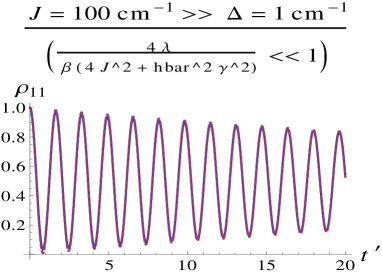
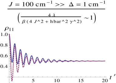
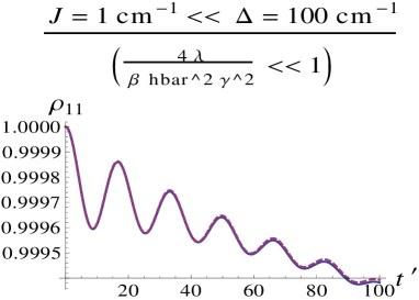
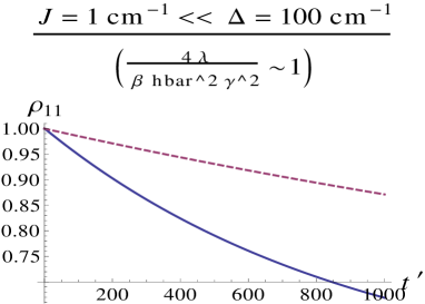
Figure 1: Verification of the analytic inequalities (Table I). Time evolution of population on site 1: blue (solid) curve is the non-Markovian solution and red (dotted) curve is the Markovian approximation. Upper row (case $J>>\Delta$): $\frac{4\lambda}{\beta(4J^{2}+\hbar^{2}\gamma^{2})}=0.04<<1,~{}~{}\lambda=2$ (upper left graph), and $\frac{4\lambda}{\beta(4J^{2}+\hbar^{2}\gamma^{2})}=0.9\sim 1,~{}~{}\lambda=50$(upper right graph). Lower row (case $J<<\Delta$): $\frac{4\lambda}{\beta\hbar^{2}\gamma^{2}}=0.02<<1,~{}~{}\lambda=2$ (lower left graph), and $\frac{4\lambda}{\beta\hbar^{2}\gamma^{2}}\sim 3,~{}~{}\lambda=10$ (lower right graph). Clearly, graphs are in accord with Table I. Time $t^{\prime}$ is the dimensionless time, $10$ units on this scale are equivalent to one ps.

V.3 Computational Results

In other parameter regimes, the validity of the Markov approximation [Eq. (22)] must be determined by numerical comparisons with the exact result [Eq. (20)]. Figure 2 compares the solution for the Markovian master equation to the non-Markovian results for the standard electronic coupling parameter values in photosynthetic EET: $\gamma^{-1}=100~{}\textrm{fs},~{}~{}J=50~{}\textrm{cm}^{-1},~{}~{}\Delta=100~{}\textrm{cm}^{-1},~{}~{}T=300~{}$K , a regime in which the estimates in Table I do not apply. The initial excitation is assumed to be on site one. The Markovian approximation is seen to be very good for $\lambda=1~{}\textrm{cm}^{-1}$, fair for $\lambda=2~{}\textrm{cm}^{-1}$ and invalid for reorganization energies $\lambda\geq 10~{}\textrm{cm}^{-1}$.

To explore regimes of validity of the Markovian approximation for other values of the physical constants, we present sample results in Figs. 3 and 4, obtained by varying $(J,\lambda)$ and $(\gamma^{-1},\lambda)$, keeping $\Delta=100$ cm^-1. The results show for these cases that the Markovian approximation is poor for large $\lambda$ and “small’ $J$ and for large $\gamma^{-1}$ and small $\lambda$. Other parameter values can be readily examined computationally using this approach.

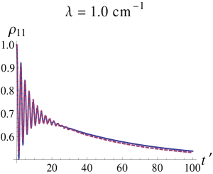
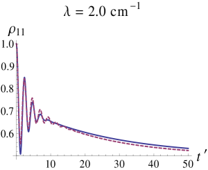
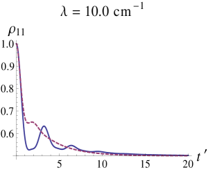
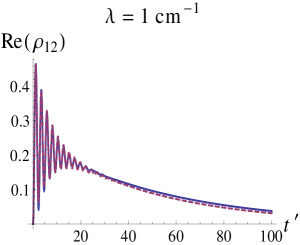
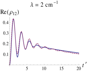
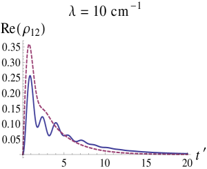
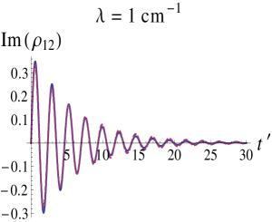
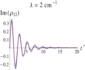
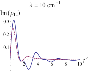
Figure 2: Time evolution of population on site 1 [$\rho_{11}(t)$] and the coherences [$\rho_{12}(t)$] [blue (solid) curve is the non-Markovian solution and red (dotted) curve is the Markovian approximation], for various values of $\lambda$ (in cm^-1). Other parameter are: $\Delta=100cm^{-1},~{}~{}J=50cm^{-1},~{}~{}\gamma=10^{13}sec^{-1}$. The breakdown of the Markov approximation at $\lambda=10~{}$cm^-1 is clearly visible. The time $t^{\prime}$ is dimensionless, with 10 units on this scale being equivalent to one ps.

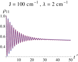
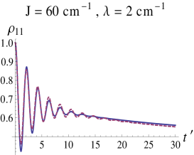
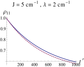
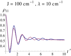
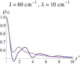
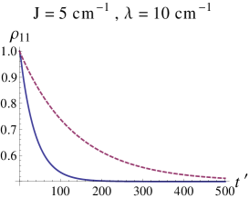
Figure 3: Time evolution of population on site 1: blue (solid) curve is the non-Markovian solution and red (dotted) curve is the Markovian approximation) for various values of the reorganization energy $\lambda$ and inter-site coupling $J$. The level separation $\Delta=100~{}\textrm{cm}^{-1}$ and $\gamma^{-1}=100$ fs. It is clear that Markovian approximation is poor for large $\lambda$ and small $J$. Time $t^{\prime}$ is the dimensionless time, $10$ units on this scale are equivalent to one ps.

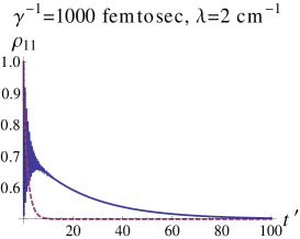
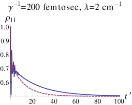
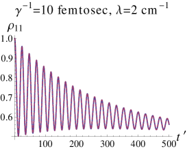
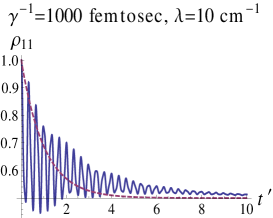
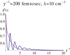
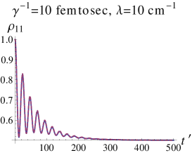
Figure 4: Time evolution of population on site 1 [blue (solid) curve is the non-Markovian solution and red (dotted) curve is the Markovian approximation] for various values of the reorganization energy $\lambda$ and phonon relaxation time $\gamma^{-1}$. The level separation $\Delta=100~{}\textrm{cm}^{-1}$ and $J=50~{}\textrm{cm}^{-1}$. It is clear that Markovian approximation is poor for large relaxation times $\gamma^{-1}$ and small $\lambda$, and it better for small $\gamma^{-1}$. $t^{\prime}$ is the scaled time, as in the figure above.

VI Regime of validity of the second-order approximation

We have considered the master equation up to the second order in system-bath interaction. The aim of this section is to determine the system-bath interaction energy range (as represented by the reorganization energy $\lambda$) over which the second order master equation [or coupled system of equations (Eq. (20)] can be used. To do so we compare estimates of the second order and the fourth order terms. This can be done analytically for the parameter regime where $J\sim\Delta$. To do so we note that up to the second order, with the master equation written in dimensionless time form [Eq. (20)], the magnitude of the second order term is of the order of $\frac{\lambda}{\beta\hbar^{2}\gamma^{2}}$ for the case $J\sim\Delta$. This arises by noting that $|H_{SR}|^{2}\sim\lambda$, and the integral $\int_{0}^{t^{\prime}}d\tau^{\prime}e^{\tau^{\prime}-t^{\prime}}\left[\cos[\frac{E_{12}}{\gamma}(t^{\prime}-\tau^{\prime})]\tilde{y}_{1}(\tau^{\prime})+\eta_{2}\sin[\frac{E_{12}}{\gamma}(t^{\prime}-\tau^{\prime})]\tilde{y}_{2}(\tau^{\prime})\right]\sim 1$, for the standard set of parameters ($\gamma^{-1}=100~{}\textrm{fs},~{}~{}J=20~{}\textrm{cm}^{-1},~{}~{}\Delta=100~{}\textrm{cm}^{-1},~{}~{}T=300~{}$K).

Similarly, we can estimate the parameter dependence of the fourth order term. To estimate this we recall the Nakajima-Zwanzig master equation (valid to all orders)

$$\frac{\partial\hat{\rho}^{I}(t)}{\partial t}=-\int_{0}^{t}d\tau tr_{R}\left(\mathcal{L}_{SR}^{I}\mathcal{S}(t,\tau)\mathcal{Q}\mathcal{L}_{SR}^{I}(\tau)\hat{R}_{eq}\right)\hat{\rho}^{I}(\tau).$$ (29)

where the time evolution operator is

$$\mathcal{S}(t,\tau) \equiv \mathcal{T}^{\rightarrow}\exp[-i\int_{\tau}^{t}d\tau^{\prime}\mathcal{Q}\mathcal{L}_{SR}^{I}(\tau^{\prime})]$$ (30)

$$= 1-i\int_{\tau}^{t}d\tau^{\prime}\mathcal{Q}\mathcal{L}_{SR}^{I}(\tau^{\prime})-\int_{\tau}^{t}d\tau_{2}\int_{\tau}^{\tau_{2}}d\tau_{1}\mathcal{Q}\mathcal{L}_{SR}^{I}(\tau_{2})\mathcal{Q}\mathcal{L}_{SR}^{I}(\tau_{1})+...$$

Here, $\mathcal{Q}=I-\mathcal{P}$ is the well know projection operator and $\mathcal{L}_{SR}^{I}$ is the system-bath Liouvillian ($-\frac{i}{\hbar}[H_{SR}^{I},.]$). The time ordering operator $\mathcal{T}^{\rightarrow}$ orders time dependent operators from left to right with decreasing time arguments, to take into account the non-commutation of operators at different times.

The zeroth order approximation to the time evolution operator $\mathcal{S}(t,\tau)$ gives the second order quantum master equation, the first order approximation to the time evolution operator gives the third order contribution which vanishes as the bath average of odd bath operators vanish (see Ref. hpb ), and the second order approximation to $\mathcal{S}$ gives the fourth order contribution. In order to estimate the magnitude of the latter term we write the fourth order term A₄ from Nakajima-Zwanzig equation as

$$\textrm{A}_{4}=\frac{1}{\hbar^{4}}\int_{0}^{t}d\tau\int_{\tau}^{t}d\tau_{2}\int_{\tau}^{\tau_{2}}d\tau_{1}tr_{R}\left\{[H_{SR}^{I}(t),\mathcal{Q}[H_{SR}^{I}(\tau_{2}),\mathcal{Q}[H_{SR}^{I}(\tau_{1}),\mathcal{Q}[H_{SR}^{I}(\tau),R_{eq}\hat{\rho}(\tau)]]]]\right\}.$$ (31)

We start from the interior commutator $(1-\mathcal{P})[H_{SR}^{I}(\tau),R_{eq}\hat{\rho}(\tau)]$ and recall that $\mathcal{P}\hat{O}=R_{eq}tr_{R}{\hat{O}}$ and $H_{SR}^{I}=V_{i}^{I}u_{i}^{I}$ (where the summation convection is used). The bath average of single bath operators vanish [$tr_{R}(u_{j}(\tau)R_{eq})=0$] so that $\mathcal{Q}$ times the interior commutator gives $[V_{i}^{I}(\tau)u_{i}(\tau),R_{eq}\hat{\rho}(\tau)]$. Similarly, writing $\mathcal{Q}=1-\mathcal{P}$ for the second from the interior commutator, and simplifying, the bath trace operation gives us the two time bath correlation functions $\langle u_{i}(\tau)u_{i}(\tau_{1})\rangle_{R}$. Repeating the same operations for the remaining commutators, noting that the bath averaging for the odd bath operators vanish and using the Wick theorem $\langle u_{i}u_{j}u_{k}u_{l}\rangle_{R}=\langle u_{i}u_{j}\rangle_{R}\langle u_{k}u_{l}\rangle_{R}+\langle u_{i}u_{k}\rangle_{R}\langle u_{j}u_{l}\rangle_{R}+\langle u_{i}u_{l}\rangle_{R}\langle u_{j}u_{k}\rangle_{R}$, we obtain that the fourth order term includes the product of two time bath correlation functions i.e., $\langle u_{i}(\tau)u_{i}(\tau_{1})\rangle_{R}\langle u_{j}(\tau_{1})u_{j}(\tau_{2})\rangle_{R}$. On converting the equation into dimensionless time form as described in Section IV, and using the high temperature approximation for the correlation function, we conclude that the order-of-magnitude of the fourth order term is;

$$\textrm{A}_{4}\sim\frac{\lambda^{2}}{\gamma^{4}\beta^{2}\hbar^{4}}.$$ (32)

The ratio $R_{42}$ of the fourth-order term to the second-order term is therefore $R_{42}=\frac{\lambda}{\gamma^{2}\beta\hbar^{2}}$, which is of the order of $0.074$ for $\lambda=1~{}\textrm{cm}^{-1}$, and $\sim 0.74$ for $\lambda=10~{}\textrm{cm}^{-1}$. This suggests that the second order approximation for the master equation is good for $\lambda\sim 1$ for the standard set of parameters ($\gamma^{-1}=100~{}\textrm{fs},~{}~{}J=20~{}\textrm{cm}^{-1},~{}~{}\Delta=100~{}\textrm{cm}^{-1},~{}~{}T=300~{}$K). However, for large $\lambda\sim 10$ the fourth order term cannot be neglected. Interestingly, the domain of applicability of the second-order approximation in this $J\sim\Delta$ regime has a dependence on the same collection of parameters, $(\lambda/\gamma^{2}\beta\hbar^{2}$ small), as does the Markov approximation in the $J\ll\Delta$.

VII Initial state preparation by an ultra-short laser pulse

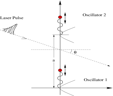
Figure 5: Two harmonic oscillators excited by an ultra-short laser pulse.

VII.1 Formulation

To understand the effect of initial coherences on the subsequent quantum dynamics, we consider a model of two 1-D harmonic oscillators separated by a distance $a$ that are excited by an ultra short laser pulse (Fig. 5). The results of this excitation are used below as sample coherent initial conditions for dimer propagation. Note that we restrict attention, as do most treatments of excitation of light-harvesting systems, to the “one-exciton manifold”, i.e. single excitations on each site. This model is useful to examine the dynamics, but should be augmented by excitation of states with bi-excitons of examining issues like entanglement, where the contributions from higher exciton states, no matter how small in magnitude, affect the entanglement measure.

In the system (Fig. 5) the wave vector of the laser pulse along the propagation direction makes an angle $\theta$ with the line perpendicular that joining the oscillators. The laser field is treated semiclassically with the field sufficiently weak to allow first order perturbation theory for the light-oscillator interaction schiff . The total Hamiltonian in the coordinate representation is then

$$H_{T} = H_{sys}+H_{int}$$

$$H_{sys} = -\frac{\hbar^{2}}{2m}\frac{\partial^{2}}{\partial y_{1}^{2}}+\frac{1}{2}k_{1}y_{1}^{2}-\frac{\hbar^{2}}{2m}\frac{\partial^{2}}{\partial y_{2}^{2}}+\frac{1}{2}k_{2}y_{2}^{2}$$

$$H_{int} = \frac{ie\hbar}{2mc}\bf{A}.\bf{\nabla}$$

$${\bf{A}}.{\bf{\nabla}} = A_{1}(y_{1},\theta,t)\hat{\epsilon}.\hat{j}\frac{\partial}{\partial y_{1}}+A_{2}(y_{2},\theta,a,t)\hat{\epsilon}.\hat{j}\frac{\partial}{\partial y_{2}}~{},$$ (33)

with the vector potential ${{\bf A}(y,\theta,t)}=\sum_{{\bf{k}}}\hat{\epsilon}_{\bf{k}}(A_{k}e^{i(ky\sin\theta-\omega t)}+A_{k}^{\ast}e^{-i(ky\sin\theta-\omega t)})$. For a coherent laser pulse, $\hat{\epsilon}_{\bf k}=\hat{\epsilon}$. If $A^{\ast}(-\frac{\omega}{c})=A(\frac{\omega}{c})$, where $c$ is the speed of light, then changing the summation to integration assuming continuous distribution of modes, we have

$${\bf A}(y,\theta,t)=\hat{\epsilon}\int_{-\infty}^{\infty}d\omega A(\omega/c)\exp[i\omega(y\sin(\theta)/c-t)].$$ (34)

For a Gaussian pulse $A(\omega/c)=A_{0}\exp[-\eta(\omega-\omega_{0})^{2}]$, where $\omega_{0}$ is the central pulse frequency and $\eta$ defines the pulse width. The vector potentials take the form

$$A_{1}(y_{1},\theta,t)= A_{0}\sqrt{\frac{\pi}{\eta}}~{}\exp\left[i\omega_{0}\left(\frac{y_{1}\sin\theta}{c}-t\right)\right]\exp\left[-\frac{1}{4\eta}\left(\frac{y_{1}\sin\theta}{c}-t\right)^{2}\right]$$

$$A_{2}(y_{1},\theta,a,t)= A_{0}\sqrt{\frac{\pi}{\eta}}\exp\left[i\omega_{0}\left(\frac{y_{2}\sin\theta}{c}-\frac{a}{c}\sin(\theta)-t\right)\right]$$ (35)

$$\exp\left[-\frac{1}{4\eta}\left(\frac{y_{2}\sin\theta}{c}-\frac{a}{c}\sin(\theta)-t\right)^{2}\right]$$

The laser frequency is assumed tuned so as to excite the first excited state, with both oscillators initially (at $t=-\infty$) in their ground states.

The eigensystems of oscillators 1 and 2 are

$$E_{n}^{(1)}=\hbar\omega_{c1}(n+1/2),~{}~{}u_{0}^{(1)}=\frac{\sqrt{\alpha_{1}}}{\pi^{1/4}}\exp[-\frac{1}{2}\alpha_{1}^{2}y_{1}^{2}],~{}~{}~{}u_{1}^{(1)}=\frac{\sqrt{2}}{\pi^{1/4}}\alpha_{1}^{3/2}y_{1}\exp[-\frac{1}{2}\alpha_{1}^{2}x_{1}^{2}]$$

$$E_{n}^{(2)}=\hbar\omega_{c2}(n+1/2),~{}~{}u_{0}^{(2)}=\frac{\sqrt{\alpha_{2}}}{\pi^{1/4}}\exp[-\frac{1}{2}\alpha_{2}^{2}y_{2}^{2}],~{}~{}~{}u_{1}^{(2)}=\frac{\sqrt{2}}{\pi^{1/4}}\alpha_{2}^{3/2}y_{2}\exp[-\frac{1}{2}\alpha_{2}^{2}y_{2}^{2}].$$ (36)

with $\omega_{ci}=\sqrt{k_{i}/m}$ and $\alpha_{i}^{4}=mk_{i}/\hbar^{2},~{}~{}i=1,2$. The total wavefunction of the system is

$$\Psi(y_{1},y_{2},t)=\sum_{m,n}a_{mn}(t)u_{n}^{(1)}(y_{1})u_{m}^{(2)}(y_{2})\exp[-\frac{i}{\hbar}(E_{n}^{(1)}+E_{m}^{(2)})t],~{}~{}~{}~{}a_{mn}(t=-\infty)=\delta_{n0}\delta_{m0}.$$ (37)

Standard first-order perturbation theory gives the coefficients as

$$a_{nm}(t)=\frac{e\cos\theta}{2mc}\int_{-\infty}^{t}dt^{\prime}\int_{-\infty}^{+\infty}dx_{1}\int_{-\infty}^{+\infty}dx_{2}u_{n}^{(1)}(x_{1})u_{m}^{(2)}(x_{2})$$

$$\times\left(A_{1}(x_{1},\theta,t^{\prime})(\frac{\partial}{\partial x_{1}})+A_{2}(x_{2},\theta,a,t^{\prime})(\frac{\partial}{\partial x_{2}})\right)u_{0}^{(1)}(x_{1})u_{0}^{(2)}(x_{2})\exp[-i\omega_{nm}t^{\prime}]$$ (38)

Using the dipole approximation, the spatial integrals for both $a_{01}$ and $a_{10}$ can be done exactly. The remaining time integral is treated as follows: the laser pulse is assumed to be ultrashort compared to the subsequent quantum dynamics. For times much greater than $t/\sqrt{\eta}$, the exponential $e^{-(t^{2}/4\eta)}$ in time integration will be small, and the upper limit of the time integration can be extended to $+\infty$. The integration can then be performed exactly, giving

$$a_{10}=-\zeta\sqrt{\mu}\cos\theta e^{-\eta\omega_{0}^{2}(1+\nu_{10})^{2}}~{}~{},$$

$$a_{01}=-\zeta\frac{\cos\theta}{\sqrt{\mu}}e^{-\eta\omega_{0}^{2}(1+\nu_{01})^{2}}.$$ (39)

Here $\mu=\alpha_{1}/\alpha_{2}=(k_{1}/k_{2})^{1/4},~{}~{}\zeta=\pi A_{0}e\sqrt{\alpha_{1}\alpha_{2}}/{\sqrt{2}}mc,~{}~{}\nu_{01}=\omega_{01}/\omega_{0},~{}~{}\nu_{10}=\omega_{10}/\omega_{0}$, with $\omega_{mn}=(E_{0}^{(1)}+E_{0}^{(2)}-E_{m}^{(1)}-E_{n}^{(2)})/\hbar$.

The first excited states of the both oscillators ($E_{1}^{(1)},~{}~{}E_{1}^{(2)}$) constitute our relevant system (they are separated by about 100 cm^-1 in typical systems like FMO), and quantum dynamics takes place between them. The superposition of the excited states is written as

$$|\psi\rangle=a_{10}|10\rangle+a_{01}|01\rangle,$$ (40)

where $|10\rangle$ indicates that the first oscillator is excited and the second is in the ground state. The density matrix at the initial time is

$$\rho_{0}=|\psi\rangle\langle\psi|=|a_{10}|^{2}|10\rangle\langle 10|+|a_{01}|^{2}|01\rangle\langle 01|+a_{10}a_{01}^{\ast}|10\rangle\langle 01|+a_{01}a_{10}^{\ast}|01\rangle\langle 10|.$$ (41)

This initial density matrix corresponds to a particular orientation angle $\theta$. For excitation of an ensemble we average over theta,

$$\langle\rho_{0}\rangle_{\theta}\equiv\frac{1}{2\pi}\int_{0}^{2\pi}\rho_{0}d\theta,$$ (42)

with the normalization

$$\rho_{11}+\rho_{22}\equiv\langle|a_{10}|^{2}\rangle_{\theta}+\langle|a_{01}|^{2}\rangle_{\theta}=1.$$ (43)

Thus,

$$\rho_{11} = \frac{\langle|a_{10}|^{2}\rangle_{\theta}}{\langle|a_{10}|^{2}\rangle_{\theta}+\langle|a_{01}|^{2}\rangle_{\theta}}$$

$$\rho_{22} = \frac{\langle|a_{01}|^{2}\rangle_{\theta}}{\langle|a_{10}|^{2}\rangle_{\theta}+\langle|a_{01}|^{2}\rangle_{\theta}}$$

$$\rho_{12} = \rho_{21}^{*}=\frac{\langle a_{10}a_{01}^{\ast}\rangle_{\theta}}{\langle|a_{10}|^{2}\rangle_{\theta}+\langle|a_{01}|^{2}\rangle_{\theta}}.$$ (44)

with

$$\langle|a_{10}|^{2}\rangle_{\theta} = \frac{1}{2}\zeta^{2}\mu e^{-2\eta\omega_{0}^{2}(1+\nu_{10})^{2}},~{}~{}~{}\langle|a_{01}|^{2}\rangle_{\theta}=\frac{1}{2}\zeta^{2}\frac{1}{\mu}e^{-2\eta\omega_{0}^{2}(1+\nu_{01})^{2}}$$

$$\langle a_{10}a_{01}^{\ast}\rangle_{\theta} = \frac{c}{a\omega_{01}}\zeta^{2}J_{1}(\frac{a\omega_{01}}{c})e^{-\eta\omega_{0}^{2}[(1+\nu_{10})^{2}+(1+\nu_{01})^{2}]}.$$ (45)

Here $J_{1}(.)$ is the Bessel function of first kind and of order $1$. This constitutes the initial density matrix for the relevant system.

VII.2 Numerical Results

Let $\eta=10^{-4}$ ps², the separation between the two oscillators $a=2$  nm,  $\omega_{01}=-\omega_{c2}=-10^{14}$ Hz, and $\omega_{10}=\sqrt{\mu}\omega_{01}$. Figure 6 shows the density matrix elements [i.e. the initial state given by Eqs. (44) and (45)] as a function of the ratio of oscillator for constants $k_{1}/k_{2}$ for various values of the excitation laser frequency.

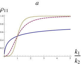
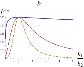
Figure 6: (a) Population of angle averaged energy state $|10\rangle\langle 10|$, and (b) Coherence $\rho_{12}$ as a function of $\mu=\frac{k_{1}}{k_{2}}$. Solid line, laser frequency $\omega_{0}=10^{14}$Hz, dashed line $5\times 10^{14}$ Hz (Orange), dotted line $10^{15}$ Hz. Note that Im$\rho_{12}=0$.

This initial state can then be used as a model for the initial conditions for the numerical solution of the non-Markovian equations [Eq. (15)] for the dimer. Figure 7 (in the site representation) compares the time evolution of $\rho_{11}(t)$ for an initial “no-coherence” state (only populations) and the model generated state with “initial coherence”, for various values of $k_{1}/k_{2}$.

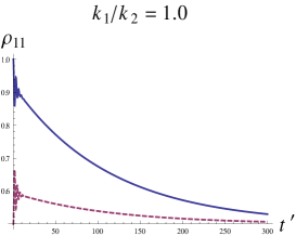
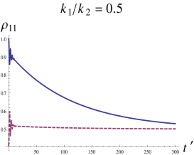
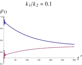
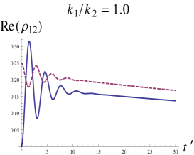
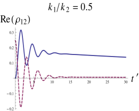
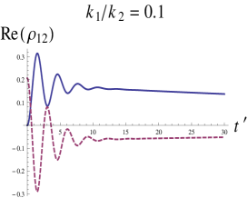
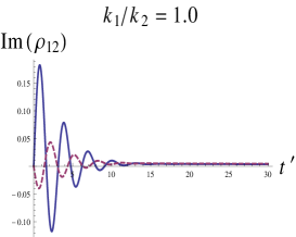
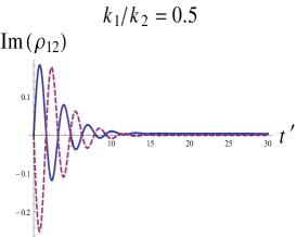
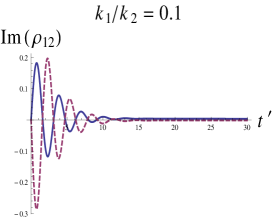
Figure 7: The effect of initial coherence on the of relaxation dynamics. Long time behavior for various values of $k_{1}/k_{2}$. Here $\lambda=1$ cm^-1 and $\omega_{0}=10^{14}$. The blue (solid) curve is for “no-coherence” initial condition , and red (dotted) curve is for the “initial coherence” condition, i.e., initial value of the density matrix elements for the model photo-excitation studied above. The second and third row shows the dynamics of the off-diagonal elements.

One may identify two time scales associated with the electronic energy transfer, the time scale over which the site occupation $\rho_{11}$ becomes relatively constant, and the rate at which this occurs. From the plots of $\rho_{11}$ in Fig. 7, it appears that the presence of initial coherence ( at $t=0$) effects both of these time scales, but has little effect on the overall damping-out of the coherence, i.e. the overall decay of oscillations in both the real and imaginary parts of $\rho_{1,2}$. By contrast, the fall-off rate for the decay of $\rho_{11}$ is far faster for the case with initially no-coherence than it is for the case where there initially is coherence. In cases other than $k_{1}/k_{2}=1.0$ the time at which the system reaches the equilibrium value of 1/2 seems similar in both the cases where there is coherence initially and where there is not.

VIII Conclusion

A straightforward approach to solving the second order Born master equation, with and without the Markov approximation, has been introduced. In addition to obtaining numerical results showing the range of validity of these approximations, a number of analytical estimates, shown in Table I, of parameter ranges over which these approximations can be used has been obtained. For the case of the traditional dimer model for electronic energy transfer in photosynthesis, surprisingly small reorganization energies (a few cm^-1) are required for the validity of the Markovian approximation. In addition, we note that for dimer coupling strengths on the order of the energy difference between site energies, higher order terms than second order in the system-bath coupling are required if $4\lambda/(\hbar^{2}\beta\gamma^{2})<<1$ is not satisfied, where $\lambda$ is the reorganization energy, and $\gamma$ defines the exponential falloff rate of the bath correlation function. Once again, the limitation to small reorganization energies, not well appreciated in the past, is made explicit.

We have also provided an example of the role of initial coherences in the subsequent evolution of the dimer dynamics for typical parameters associated with model photosynthetic light harvesting systems.

IX Acknowledgment

Financial support from the Natural Sciences and Engineering Research Council of Canada and from the U.S. Air Force Office of Scientific Research under grant number FA9550-10-1-0260 is gratefully acknowledged.

References

• (1) V. May and O. Kuhn, Charge and Energy Transfer Dynamics in Molecular Systems (Wiley-VCH, New York, 2004).
• (2) H.-P. Breuer and F. Petruccione, The Theory of Open Quantum Systems (Oxford University Press, New York, 2002).
• (3) M. Schlosshauer, Decoherence and the Quantum to Classical TransitionSpringer, New York, 2008
• (4) M. Shapiro and P. Brumer, Principles of the Quantum Control of Molecular ProcessesWiley, New York, 2003; M. Shapiro and P. Brumer, Quantum Control of Molecular Processes Wiley-VCH, New York, in press;
• (5) G. S. Engel, T. R. Calhoun, E. L. Read, T. K. Ahn, T. Mancal, Y.-C. Cheng, R. E. Blankenship and G. R. Fleming, Nature 446, 782 (2007); H. Lee, Y. C. Cheng, G. R. Fleming, Science 316, 1462 (2007); E. Collini, G. D. Scholes, Science 323, 369 (2009); E. Collini, C. Y. Wong, K. E. Wilk, P. M. G. Curmi, P. Brumer and G. D. Scholes, Nature 463, 644 (2010).
• (6) A. Ishizaki and G. R. Fleming, J. Chem. Phys. 130, 234110 (2009).
• (7) T. Förster, Ann. Phys. 437, 55 (1948); R. Silbey, Annu. Rev. Phys. Chem. 27, 203 (1976).
• (8) H. Van Amerongen, L. Valkunas and R. Van Grondelle, Photosynthesis Excitons (World Scientific, Singapore, 2000); R. E. Blankenship, Molecular Mechanisms of Photosynthesis (World Scientific, London, 2002).
• (9) V. M. Kenkre and R. S. Knox, Phys. Rev. B. 9, 5279 (1974).
• (10) V. M. Kenkre, Phys. Rev. B. 12, 2150 (1975).
• (11) M. B. Plenio and S. F. Huelga, New J. Phys. 10, 113019 (2008).
• (12) M. Sarovar, Y.-C. Cheng and K. B. Whaley (2009).
• (13) M. Sarovar, A. Ishizaki, G. R. Fleming and K. B. Whaley, Nat. Phys. 6 462 (2010)
• (14) A. Ishizaki and G. R. Fleming, New J. Phys. 12 (2010) 055004.
• (15) F. Caruso, A. W. Chin, A. Datta, S. F. Huelga and M. B. Plenio, Phys. Rev. A 81, 062346 (2010).
• (16) F. Fassiolo, A. Olaya-Castro, New J. Phys. 12, 085006 (2010).
• (17) M. Mohseni, P. Rebentrost, S. Lloyd and A. Aspuru-Guzik, J. Chem. Phys. 129, 174106 (2008).
• (18) P. Rebentrost, M. Mohseni and A. Aspuru-Guzik, J. Phys. Chem. B 113, 9942 (2009).
• (19) S. Jang, Y. Cheng, D. R. Reichman and J. D. Eaves, J. Chem. Phys. 129, 101104 (2008).
• (20) A. Ishizaki and G. R. Fleming, J. Chem. Phys. 130, 234111 (2009); Y. Tanimura and R. Kubo, J. Phys. Soc. Jpn. 58, 101 (1989).
• (21) A short description of the technique is outlined in N. Singh and P. Brumer, Faraday Discuss. 153 (in press).
• (22) L. I. Schiff, Quantum Mechanics, (McGraw-Hill, N.Y. , 1968)