Local Moment Formation of an Anderson Impurity on Graphene

Abstract

We study the property of a magnetic impurity on a single-layer graphene within an Anderson impurity model. Due to the vanishing local density of states at the Fermi level in graphene, the impurity spin cannot be effectively screened out. Treating the problem within the Gutzwiller approximation, we found a region in the parameter space of $U$-$E^{f}$ where the impurity is in the local moment state, which is characterized by a zero effective hybridization between the bath electron and the magnetic impurity. Here $U$ is the onsite Coulomb repulsion of the impurity electrons and $E^{f}$ the impurity energy level. The competition between $U$ and $E^{f}$ is also discussed. While larger $U$ reduces double occupation and favors local moment formation, a deeper impurity level prefers double occupation and a nonzero hybridization and thus a Kondo screened state. For a fixed $U$, by continuously lowering the impurity level, the impurity first enters from a Kondo screened state into a local moment state and then departs from this state and re-enters into the Kondo screened state.

I Introduction

The research on a single layer of graphite – graphene – has been advanced tremendously after its successful exfoliation, Novoselov et al. (2004) the importance of which cannot be overstated. Due to its exceptional electronic, thermal, and mechanical properties, graphene virtually finds its potential in every aspect of modern technology. For example, it could have tremendous applications in microelectronics due to its high electron mobility. It also has a great deal of potential in spintronics, Son et al. (2006); Moghaddam and Zareyan (2010) where the spin current is utilized. From the theoretical perspective, it has been a test ground for many fundamental physics laws due to its similarity to massless Dirac fermions, Semenoff (1984); DiVincenzo and Mele (1984) where the “speed of light” is replaced by the graphene Fermi velocity $v_{F}\sim 10^{6}\nicefrac{\mathrm{m}}{\mathrm{s}}$.

The property of a magnetic impurity in a metallic host is an important problem in condensed matter physics. In a conventional metal, the Kondo effect, where the itinerant electrons completely screen the magnetic moment of the impurity, is always present at low temperatures. The impurity property is not sensitive to the detailed band structure of the host metal. The most important element from the impurity bath is its density of states (DOS) at the Fermi level, $\rho(\omega=0)$, and it enters the physics through the scattering rate $\Gamma=\rho(0)V$, with $V$ being the hybridization matrix between the impurity and host electrons. This is due to the fact that in conventional metals, the DOS around the Fermi energy is almost a finite constant. However, it has been theoretically found that vanishing host DOS (power law or otherwise) could lead to significant changes to the Kondo physics. Withoff and Fradkin (1990); Bulla et al. (1997) The main finding, among many others, is that the small available states around $\omega=0$ for conduction electrons makes the effective hybridization between the band electron and the impurity vanishingly small. This ineffective screening of the impurity moment causes the impurity to decouple from the conduction media and form a free local moment (LM). Withoff and Fradkin Withoff and Fradkin (1990) found that the Kondo coupling, $J$, has to be larger than some critial value for the Kondo effect to take place. However, the dependence of the magnetic impurity state on the conduction electron DOS is a tricky one. For exmaple, numerical renormalization group calculation shows that the impurity state depends not only on the index of a power law DOS but also on the size of this power law region. Gonzalez-Buxton and Ingersent (1998)

The hexagonal structure of graphene has two inequivalent carbon atoms, A and B, in one unit cell. In the tight bind approximation, the graphene electronic structure is modelled by a nearest neighbor hopping integral $t$. Further neighboring hopping integrals are small and are usually neglected. The conduction and valence bands then touch at the corners of the graphene Brillouin zone, $\mathbf{K}$ and $\mathbf{K}^{\prime}$, which are called the Dirac points. The dispersion near these Dirac points is linear in $\mathbf{k}$ and the DOS is also linear in energy. For all practical purposes, this tight binding description is quite accurate. Many peculiar properties of graphene are closely related to this linear dispersion and the corresponding linear DOS at low energies. AHCastroNeto:2009 The state of a magnetic impurity on graphene is expected to be very different from that on an ordinary metal. However, the existence of two inequivalent Dirac points could also complicate the simple linear DOS argument since this may lead to multi-channel Kondo effect. Zhu et al. (2010) The specific problem of a magnetic impurity on graphene has recently been studied by several groups. Uchoa et al. (2008); Zhuang et al. (2009); Cornaglia et al. (2009); Jacob and Kotliar (2010); MVojta2010 Besides its theoretical importance as a prototypical many-body toy model, it is also important to understand magnetic impurities on graphene from the application perspective. It was observed that introduction of vacancies into graphite or graphene could indeed induce ferromagnetism. Esquinazi et al. (2003); Ohldag et al. (2007); Barzola-Quiquia et al. (2007); Chen et al. (2010)

In this paper, we explore the properties of a magnetic impurity in a single-layer graphene within an Anderson impurity model. Within the Gutzwiller approximation, we are able to obtain a phase diagram within the parameter space spanned by the impurity level and on-site Hubbard repulsion. We identify a parameter region, where local moment is formed on the impurity. In addition, a re-entrant Kondo resonance behavior is found. The effect of graphene chemical potential, $\mu$, is also discussed.

The outline of the paper is as follows: In Sec. II, the model Hamiltonian for an Anderson impurity in the graphene is introduced. The Gutzwiller procedure toward the solution is explained. In Sec. III, we present the results on the local moment formation and Kondo resonance state as a result of the competition between the impurity level and on-site Hubbard repulsion. Finally, a summary is given in Sec. IV.

II Model Hamiltonian and Theoretical Method

We start with a single-impurity Anderson model in graphene. The Hamiltonian is partitioned into three parts— the pristine graphene subsystem $\hat{H}_{0}$, the impurity subsystem $\hat{H}_{\rm imp}$, and the hybridization $\hat{H}_{\rm hyb}$ between these two subsystems, that is,

$$\mathcal{H}=\hat{H}_{0}+\hat{H}_{\rm imp}+\hat{H}_{\rm hyb}\;,$$ (1)

where the three parts can be written out explicitly,

$$\hat{H}_{0}= -t\sum_{\mathbf{k}\sigma}\xi(\mathbf{k})a_{\mathbf{k}\sigma}^{\dagger}b_{\mathbf{k}\sigma}+\mathrm{H.c.}\;,$$ (2a)

$$H_{\rm imp}= \sum_{\sigma}E^{f}f_{\sigma}^{\dagger}f_{\sigma}+Uf_{\uparrow}^{\dagger}f_{\uparrow}f_{\downarrow}^{\dagger}f_{\downarrow}\;,$$ (2b)

$$H_{\rm hyb}= \frac{V}{\sqrt{\mathcal{N}}}\sum_{\mathbf{k}}a_{\mathbf{k}\sigma}^{\dagger}f_{\sigma}+\mathrm{H.c.}\;.$$ (2c)

We take a $\mathbf{k}$-independent hybridization between carbon $\pi$-electrons and the impurity spin, $V_{\mathbf{k}}=V$. Here $\xi(\mathbf{k})=\sum_{i=1}^{3}\mathrm{e}^{\mathrm{i}\mathbf{k}\cdot\mathbf{\eta}_{i}}$, where $\mathbf{\eta}_{i}$, $i=1,2,3$, are the vectors connecting to the three nearest neighbors of a carbon site, and $\mathcal{N}$ is the number of unit cells. As mentioned above, $t$ is the nearest neighbor hopping integral, $t=2.7$eV. In the rest of the paper we take $t$ as the unit of energy. The impurity is taken to be at the origin of the A-sublattice. For the more general case where a magnetic adatom is considered, the impurity could be anywhere and hybridization between the impurity and its all neighboring sites should be considered. As discussed by Uchoa et al., Uchoa et al. (2011) this leads to an effective $\mathbf{k}$-dependent hybridization $V(\mathbf{k})$.

The rich physics of the Anderson impurity model comes from the on-site Hubbard interaction $U$ on the impurity. For small $U$, a Hartree-Fock approximation is usually sufficient. For the cases of intermediate to large $U$, more degrees of the correlation effect must be taken into account. Here we take a projection approach and treat $U$ in the Gutzwiller approximation. In this approximation, the effect of $U$ is taken into account by reducing the effective hybridization between the conduction electrons and the impurity electrons. For example, in the $U=\infty$ limit, the process $f_{\sigma}^{\dagger}a_{0\sigma}$ is prohibited if there is already a $\bar{\sigma}$-$f$ electron at the impurity site, while there is no such restriction if $U=0$; see Ref Zhang et al. (1988) for a detailed discussion. On the mean field level, we renormalize the hybridization strength $V$ with $\widetilde{V}_{\sigma}=g_{\sigma}V$, $g_{\sigma}\leq 1$, and replace the interaction term with $Ud$, with $d=\langle f_{\uparrow}^{\dagger}f_{\uparrow}f_{\downarrow}^{\dagger}f_{\downarrow}\rangle$. Here $g_{\sigma}$ is the Gutzwiller factor that depends on the impurity number occupation $n^{f}_{\sigma}$ ($n^{f}=n^{f}_{\uparrow}+n^{f}_{\downarrow}$ being the total impurity occupation) and double occupation $d$. The spin dependent Gutzwiller factor is,

$$g_{\sigma}=\frac{\sqrt{(1-n^{f}+d)(n^{f}_{\sigma}-d)}+\sqrt{d(n^{f}_{\bar{\sigma}}-d)}}{\sqrt{n^{f}_{\sigma}(1-n^{f}_{\sigma})}}.$$ (3)

Note that this form of $g_{\sigma}$ explicitly breaks the spin rotational invariance, which the model Hamiltonian possesses. However, in the following, we will only concern ourselves with the stability of the nonmagnetic Kondo screened state, $n_{\uparrow}=n_{\downarrow}$, and thus concentrate on the calculation where $g_{\uparrow}=g_{\downarrow}=g$. A constraint term, $\sum_{\sigma}\lambda_{\sigma}(\hat{n}_{\sigma}^{f}-n_{\sigma}^{f})$, is also added to the mean field Hamiltonian. Here the Langrange multipliers, $\lambda_{\sigma}$, serve to renormalize the impurity energy level. Although this term is formally the same to a direct Hartree decoupling of the interaction term, $\sum_{\sigma}U\hat{n}_{\sigma}^{f}n_{\bar{\sigma}}^{f}$, the self-consistency conditions are quite different, and thus would lead to different physics. It is noted that this approach is equivalent to the Kotliar-Ruckenstein slave-boson approximation, Kotliar and Ruckenstein (1986) which has been successfully applied in the study of Anderson impurity models. Savrasov et al. (2005) After the above mean field procedure, we have the renormalized hybridization and impurity Hamiltonians,

$$\widetilde{H}_{\rm hyb}=\frac{1}{\sqrt{\mathcal{N}}}\sum_{\mathbf{k}\sigma}\widetilde{V}_{\sigma}a_{\mathbf{k}\sigma}^{\dagger}f_{\sigma}+\mathrm{H.c.},$$ (4)

$$\widetilde{H}_{\rm imp}=\sum_{\sigma}\left(E^{f}+\lambda_{\sigma}\right)f_{\sigma}^{\dagger}f_{\sigma}+Ud.$$ (5)

As such, the effective non-interacting Hamiltonian is, $\widetilde{\mathcal{H}}=H_{0}+\widetilde{H}_{\rm hyb}+\widetilde{H}_{\rm imp}$. There are two major differences comparred to the Hartree-Fock mean field approximation. First, the hybridization strength $V$ is renormalized with a factor $g_{\sigma}$ that is dependent on the impurity occupation $n^{f}_{\sigma}$ and double occupation $d$, which is in turn dependent on $U$. The second difference is that the impurity level is renormalized by the Lagrange multipliers $\lambda_{\sigma}$, instead of $Un_{\bar{\sigma}}^{f}$. In the Hartree-Fock approximation, the impurity level renormalization $Un_{\bar{\sigma}}^{f}$ becomes unphysically large for large $U$.

In the limit $U\rightarrow\infty$, the double occupation $d$ should tend to zero. By looking at the form of $g_{\sigma}$ in Eq. (3), it is clear that if at the same time $n^{f}$ goes to 1, then $g_{\sigma}$ approaches zero. In this limit, the magnetic impurity and the conduction band decouples since the effective hybridization $\widetilde{V}_{\sigma}=g_{\sigma}V$ is now zero. The impurity is in the LM state. It is interesting to realize that this is analogous to the Brinkman-Rice type of metal-insulator transition in the Hubbard model at half filling, Brinkman and Rice (1970) except that here one requires “half filling” on the impurity site. Unlike the half filled Hubbard model, in addition to the chemical potential $\mu$, the impurity number occupation is also dependent on several other aspects. It obviously is a function of the impurity level $E^{f}$. It also depends on $U$, since the interaction modifies the impurity level through $\lambda_{\sigma}$. The conduction electronic structure and the hybridization $V$ also affect the impurity occupation. One can then tune these parameters so that the impurity site is half filled, and then expects to have an LM state for appropriate values of $U$, where $d=0$. It is also worth pointing out that having a state with $n^{f}=1$ does not mean that the impurity is in the LM state. The criterion is to have a zero $g_{\sigma}$. This will become apparent when we present the results below.

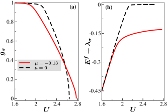
Figure 1: (Color online) The Gutzwiller factor $g_{\sigma}$ (a) and the effective impurity level $E^{f}+\lambda_{\sigma}$ (b) as a function of the on-site interaction $U$ for two different chemical potential values $\mu=0$ and $\mu=-0.13$. The impurity level is fixed at $E^{f}=-2$ and the hybridization strength is set at $V=0.52$.

We now set out to solve the effective Hamitonian $\widetilde{\mathcal{H}}$. First of all, $\widetilde{\mathcal{H}}$ is now non-interacting and can be readily solved by the usual Green function method, except that we need to take care of the self-consistency equations of $d$ and $\lambda_{\sigma}$, which are obtained by minimizing the free energy. At zero temperature, $T=0$ (on which the rest of the calculation is based), the free energy equals to the ground state energy and the self-consistency equations are obtained by taking partial derivatives of $\langle\widetilde{H}\rangle$ with respect to $d$ and $n^{f}_{\sigma}$:

$$U+V\sum_{\sigma}\frac{\partial g_{\sigma}}{\partial d}\left[\left\langle a_{0\sigma}^{\dagger}f_{\sigma}\right\rangle+\left\langle f_{\sigma}^{\dagger}a_{0\sigma}\right\rangle\right]=0,$$ (6)

$$\lambda_{\sigma}=V\sum_{\sigma}\frac{\partial g_{\sigma}}{\partial n^{f}_{\sigma}}\left[\left\langle a_{0\sigma}^{\dagger}f_{\sigma}\right\rangle+\left\langle f_{\sigma}^{\dagger}a_{0\sigma}\right\rangle\right],$$ (7)

where the expectation values $\langle\cdots\rangle$ are taken in the effective Hamiltonian $\widetilde{\mathcal{H}}$ and are determined from their respective retarded Green functions. Applying the equation of motion method, we find the following retarded Green functions,

$$G^{\mathrm{R}}_{f_{\sigma},f_{\sigma}^{\dagger}}(\omega) =\frac{1}{\omega^{+}-E^{f}-\lambda_{\sigma}-\widetilde{V}_{\sigma}^{2}G_{0}^{\mathrm{R}}(\omega)},$$ (8a)

$$G^{\mathrm{R}}_{a_{\mathbf{k}\sigma},f_{\sigma}^{\dagger}}(\omega) =\frac{\omega^{+}}{(\omega^{+})^{2}-\lvert\xi(\mathbf{k})\rvert^{2}}\widetilde{V}_{\sigma}G^{\mathrm{R}}_{f_{\sigma},f_{\sigma}^{\dagger}}(\omega),$$ (8b)

where $\omega^{+}=\omega+\mathrm{i}0^{+}$ and $G_{0}^{\mathrm{R}}(\omega)$ is the retarded Green function for the clean graphene:

$$G_{0}^{\mathrm{R}}(\omega)=\frac{1}{\mathcal{N}}\sum_{\mathbf{k}}\frac{\omega^{+}}{\left(\omega^{+}\right)^{2}-\lvert\xi(\mathbf{k})\rvert^{2}}.$$ (9)

The expectation values in Eqs. (6) and (7) and $n_{\sigma}^{f}=\langle f_{\sigma}^{\dagger}f_{\sigma}\rangle$ are then computed as $\langle O_{1}O_{2}\rangle=-\frac{1}{\pi}\int d\omega\;\mathrm{Im}G_{O_{1}O_{2}}^{\mathrm{R}}(\omega)f_{FD}(\omega-\mu)$, with $f_{FD}$ the Fermi-Dirac distribution function. For a given set of parameters, {$U$, $E^{f}$, $V$, $\mu$}, Eqs. (6) and (7) together with the form of $\widetilde{H}$ yield a set of nonlinear equations of $d$, $n^{f}_{\sigma}$ and $\lambda_{\sigma}$, which can be readily solved. The impurity DOS is given by $\rho^{f}_{\sigma}(\omega)=-\frac{1}{\pi}\mathrm{Im}\;G_{f_{\sigma},f_{\sigma}^{\dagger}}^{\mathrm{R}}(\omega)$.

III Results and Discussions

Let us first fix the impurity level $E^{f}$ and see the effect of $U$ on the impurity state. Figure 1(a) shows the Gutzwiller factor as a function of $U$ for two different cases: $\mu=0$ and $\mu=-0.13$. The impurity level is at $E^{f}=-2$. For small $U$ the Gutzwiller factor $g_{\sigma}$ is unity, which is expected, since in the non-interacting impurity situation, there should be no renormalization of the hybridization strength. As $U$ increases, $g_{\sigma}$ continuously decreases. There is a critical value of $U$, $U_{c}$, in each case where $g_{\sigma}$ is zero. At this point, the effective hybridization between the conduction electron and magnetic impurity is zero and an LM state forms. As discussed earlier, the impurity occupation has to be $n_{\sigma}^{f}=1/2$ in the LM state (see Fig. 2(a)). The formation of the impurity LM state can be envisioned from two facts: $g_{\sigma}$ approaches zero and the effective impurity level $(E^{f}+\lambda_{\sigma})\rightarrow\mu$ as $U$ goes toward $U_{c}$ (see Fig. 1(b)). From the Green function Eq. (8a), it is then clear that, if $\widetilde{V}_{\sigma}\rightarrow 0$ at the same time, the impurity DOS is narrowed to a level just at the Fermi energy. That is, the decoupling from the conduction band and the effective impurity level reaching the Fermi energy have to happen at the same time for an LM state to be realized. The LM state is stable against further increase of $U$ since the impurity is already decoupled from the conduction band. Larger $U$ will not change the double occupation, which is already at its lowest possible value $d=0$, and thus will not change the impurity occupation as can be seen from Eq. (7). Note that before the system reaches the LM state, the impurity occupation does depend on $U$ by shifting the effective impurity level through $\lambda_{\sigma}$ and in this regime $d$ is still dependent on $U$.

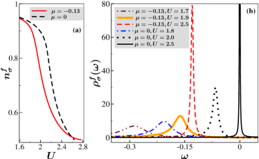
Figure 2: (Color online) (a) The impurity occupation as a function of the onsite interaction $U$ for $\mu=0$ and $\mu=-0.13$. In both cases, the spin-resolved occupation number goes to $1/2$ as $U$ approaches the critical value. (b) The resonance peak around $\mu$ for several values of $U$. The resonance peak moves progressively toward $\mu$ and the peak becomes sharper and more symmetric as $U$ is increased. The impurity level is fixed at $E^{f}=-2$ and the hybridization strength is set at $V=0.52$.

The different critical value $U_{c}$ for the two cases, $\mu=0$ and $\mu=-0.13$ suggests that graphene DOS at the Fermi level plays a central role. The graphene DOS is zero at $\mu=0$, and the hybridization between the host and impurity is inefficient to fully screen out the impurity spin. By comparison, for the $\mu=-0.13$ case, where there is a finite DOS at the Fermi level, a larger value of $U_{c}$ is needed to bring the impurity into the LM state. We can look at how the resonance peak evolve as we ramp up $U$. As shown in Fig. 2(b), the resonance peak moves toward the Fermi level and also gets sharper for increasing $U$. Due to the singularity of the graphene DOS at $\omega=\pm t$, the impurity DOS also has peaks around these energies (not shown in figure). But as $U$ increases, the weight of these states diminishes and the impurity occupation mainly comes from around the resonance energy. As the resonance peaks move from below toward the Fermi energy, they also become more symmetric, suggesting the effect of $\widetilde{V}^{2}_{\sigma}G_{00}(\omega)$ term in Eq. (8a) falls down.

Figure 3: (Color online) (a) Impurity occupation as a function of $E^{f}$ for three different values of $U$. (b) The Gutzwiller factor $g_{\sigma}$ as a function of $E^{f}$ for the same three $U$’s as in (a); $V=0.52$, $\mu=-0.13$ in both plots.

Let us now look at the effect of the impurity level. Unlike the case of varying $U$, the LM state is not stable if one lowers the impurity level past a critical value. Figure 3(a) shows the impurity occupation as a function of the impurity level for three different values of $U$. We can see that as the impurity level goes deeper inside the conduction Fermi sea, the occupation increases. It is interesting to notice that there is a flat region of the curve, where the impurity occupation seems independent of $E^{f}$ for moderate on-site Hubbard interaction $U$, for example $U=2.6$ in Fig. 3(a). The impurity occupation in this region is 1, which suggests that an LM state has possibly formed. For smaller $U$, the flat region shrinks and is slightly dependent on $E^{f}$, for example, $U=2.3$ in Fig. 3(a). However, although the curves in Fig. 3(a) look similar, the physics are fundamentally different for these different values of $U$. The large $U$ value curve represents a transition from a Kondo screened state to an LM state and then back to a Kondo state as the impurity level is further lowered, while there is no such transition for the smaller $U$ curve. This can be more convincingly seen from Fig. 3(b) where $g_{\sigma}$ is plotted against $E^{f}$ for the same values of $U$ as in Fig. 3(a). For $U=2.6$, the Gutzwiller factor $g_{\sigma}$ decreases as $E^{f}$ goes down, reaching zero at the upper critical value $E^{f}_{\rm c1}=-1.1$. Before $E^{f}$ reaches the lower critical value $E^{f}_{\rm c2}=-1.76$, the only solution to the system is the decoupled conduction band and impurity. The region between $E^{f}_{\rm c1}$ and $E^{f}_{\rm c2}$ also corresponds to the flat region where the impurity occupation is 1 in Fig. 3(a). The upper critical value $E^{f}_{\rm{c}1}$ and lower critical value $E^{f}_{\rm{c}2}$ of $E^{f}$ are identified from the zero segment in $g_{\sigma}$, which is much clearer than from the flat region of impurity occupation as in Fig. 3(a). One can also see from Fig. 3(b) that smaller $U$ does not produce an LM state for all valules of $E^{f}$: The Gutzwiller factor is always finite for $U=2.3$. There is a critical value of $U$ such that below this value there is no LM state for any value of $E^{f}$. This is identified as when $E^{f}_{\rm{c}1}=E^{f}_{\rm{c}2}=-1.35$ for $U=2.44$. Comparing Fig. 3(a) and Fig. 3(b), we see that $g_{\sigma}=0$ is a more natural and physically clear way of identifying the LM state.

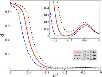
Figure 4: (Color online) Impurity double occupation $d$ as a function of the impurity level for the same three values of $U$ as in Fig. 3. Inset: Zoom in of the main figure for $E^{f}$ from -2 to 0.

The entrance and departure of the LM state upon lowering the impurity level suggests the competition between $U$ and $E^{f}$. Large $U$ would inevitably put the impurity in the no-double-occupancy state, $d=0$. In Fig. 4 we plot the double occupation, $d$, against $E^{f}$. When $E^{f}$ is close to zero, due to small available graphene electron DOS, the impurity occupation is small and thus the double occupation is also small, since $d<n^{f}_{\sigma}$. Lowering $E^{f}$ will increase $d$ by increasing the overall impurity occupation $n^{f}$. But eventually the effect of $U$ kicks in and further lowering $E^{f}$ actually makes double occupation unfavorable. As $n^{f}$ approaches 1 and $d$ goes to 0, $g_{\sigma}$ approaches 0, where we have an LM state. But further lowering $E^{f}$ favors a state, where $n^{f}$ is larger than 1. This inevitably allows double occupation and moves the impurity out of the LM state and back to the Kondo screened state again.

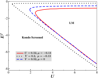
Figure 5: (Color online) The regions of LM state and Kondo screened state on the $U$-$E^{f}$ plane for different sets of $V$ and $\mu$.

Finally, we put together the effects of $U$ and $E^{f}$ on the impurity state and map out the regions of Kondo screened state and LM state on the $U$-$E^{f}$ plane. We plot the “phase diagram” of the impurity state in Fig. 5 for three sets of $(\mu,V)$. The general feature is that for moderate $U$, as we lower the impurity level, the impurity goes from the Kondo screened state to a decoupled LM state, and stays in this state until the level is low enough. At this point, the impurity and the host graphene start to talk to each other again. However, if we look along the $U$-axis, after the impurity enters the LM state, it remains in that state even if we further increase $U$. Comparing the sets of curves, we see that larger hybridization strength favors the Kondo screened state and thus gives a smaller LM region. Also, moving away from the Dirac points makes it less susceptible to LM formation.

IV Summary and Concluding remarks

In conclusion, based on the Gutzwiller approximation, we have carried out a detailed study on the LM formation of a single magnetic impurity in graphene. Due to its linear DOS near the Fermi level, graphene allows the possibility of LM formation. It has been shown that for moderate impurity level and large on-site Hubbard interaction on the impurity, an LM state is favored over a Kondo singlet state. We have explored the competition of impurity level and on-site Hubbard interaction and mapped out the LM region on the $U$-$E^{f}$ plane. We emphasize the importance of identifying the LM state by the vanishing of the effective hybridization as opposed to the unit impurity occupation, $n^{f}=1$. The effect of graphene Fermi level is also discussed. It is remarkable that the simple Gutzwiller approximation captures the essential physics in this model. The Gutzwiller approximation being a mean field approximation of the projection method does not handle the excited states very well. But as we have seen that the spetral weight of the impurity state is predominantly centered around the resonance energy. This feature justifies the applicability of the method used in this study.

The results presented here for a single Anderson impurity also remind us of the so called Kondo breakdown (KB) phenomena Pépin (2007); Paul et al. (2007) in a lattice model, where a heavy $f$ band decouples from a wider $c$ band. In the KB regime, the decoupled $f$ band would usually be polarized due to exchange interaction among the $f$-electrons. The magnetic state of the LM impurity is not determined in the single impurity case. A small magnetic field will align it in the direction of the field, due to the Zeeman energy. For more than two impurities, RKKY interaction occurs, and the magnetic state of the impurities in the LM state depends on the nature of this interaction. For example, for two impurities situated at the lattice sites the RKKY interaction could be ferromagnetic or antiferromagnetic, depending on whether they are on the same or opposite sublattice. Brey et al. (2007); Saremi (2007); Rappoport et al. (2009) The sign and strength of the RKKY interaction also depend on the graphene doping level, and whether the impurities are away from the carbon atoms. In such circumstances, the real-space Gutzwiller approximation is an ideal tool for investigating the impurity magnetic states.