Stability of precessing domain walls in ferromagnetic nanowires

Abstract

We show that recently reported precessing solution of Landau-Lifshitz-Gilbert equations in ferromagnetic nanowires is stable under small perturbations of initial data, applied field and anisotropy constant. Linear stability is established analytically, while nonlinear stability is verified numerically.

I Introduction

The manipulation and control of magnetic domain walls (DWs) in ferromagnetic nanowires has recently become a subject of intense experimental and theoretical research. The rapidly growing interest in the physics of the DW motion can be mainly explained by a promising possibility of using DWs as the basis for next-generation memory and logic devices Allwood05 ; Cowburn07 ; Parkin08 ; Hayashi08 ; Thomas10 . However, in order to realize such devices in practice it is essential to be able to position individual DWs precisely along magnetic nanowires. Generally, this can be achieved by either applying external magnetic field to the nanowire, or by generating pulses of spin-polarized electric current. The current study is concerned with the former approach.

Even though the physics of magnetic DW motion under the influence of external magnetic fields has been studied for more than half a century LandoLifshitz35 ; Gilbert55 ; SchryerWalker74 ; Kosevich90 , current understanding of the problem is far from complete and many new phenomena have been discovered only recently Hickey08 ; Wang09 ; Wang09b ; Sun10 ; our_PRL . In particular, a new regime has been reported Sun10 ; our_PRL in which rigid profile DWs travel along a thin, cylindrically symmetric nanowire with their magnetization orientation precessing around the propagation axis. In this paper we address the stability of the propagation of such precessing DWs with respect to perturbations of the initial magnetization profile, some anisotropy properties of the nanowire, and applied magnetic field.

Let $\mathbf{m}(x)=(\cos\theta(x),\sin\theta(x)\cos\phi(x),\sin\theta(x)\sin\phi(x))$ denote the magnetization along a one-dimensional wire. With easy magnetization axis along $\mathbf{\hat{x}}$ and hard axis along $\mathbf{\hat{y}}$, the micromagnetic energy is given by SS

$$E(\mathbf{m})=\mbox{$\frac{1}{2}$}\int\left(A\mathbf{m^{\prime}}^{2}+K_{1}(1-m_{1}^{2})+K_{2}m_{2}^{2}\right)\,dx\\ =\mbox{$\frac{1}{2}$}\int\left(A{\theta^{\prime}}^{2}+\sin^{2}\theta(A{\phi^{\prime}}^{2}+K_{1}+K_{2}\cos^{2}\phi)\right)\,dx$$ (1)

where $A$ is the exchange constant and $K_{1}$, $K_{2}$ the anistropy constants. Here and in what follows, integrals are taken between $-\infty$ and $\infty$ (for the sake of brevity, limits of integration will be omitted).

We consider here the case of uniaxial anisotropy, $K_{2}=0$. Minimizers of $E$ subject to the boundary conditions

$$\lim_{x\rightarrow\pm\infty}\mathbf{m}(x)=\pm\mathbf{\hat{x}},$$ (2)

describe optimal profiles for a domain wall separating two magnetic domains with opposite orientation. The optimal profiles satisfy the Euler-Lagrange equation

$$\mathbf{m}\times\mathbf{H}=0,$$ (3)

where

$$\mathbf{H}=-\frac{\delta E}{\delta\mathbf{m}}=A\mathbf{m^{\prime\prime}}+K_{1}(\mathbf{m}\cdot\mathbf{\hat{x}})\mathbf{\hat{x}}=-e_{0}\mathbf{m}+e_{1}\mathbf{n}+e_{2}\mathbf{p}.$$ (4)

Here $\mathbf{m}$, $\mathbf{n}=\partial\mathbf{m}/\partial\theta$ and $\mathbf{p}=\mathbf{m}\times\mathbf{n}$ form an orthonormal frame, and the components of $\mathbf{H}$ in this frame are given by

$$e_{0} =A{\theta^{\prime}}^{2}+\sin^{2}\theta(K_{1}+A{\phi^{\prime}}^{2})$$

$$e_{1} =A\theta^{\prime\prime}-\frac{1}{2}\sin 2\theta(K_{1}+A{\phi^{\prime}}^{2}),$$

$$e_{2} =A\sin\theta\phi^{\prime\prime}+2A\cos\theta\theta^{\prime}\phi^{\prime}.$$ (5)

In terms of these components, the energy Eq. (1) (with $K_{2}=0$) is given by

$$E(\mathbf{m})=\mbox{$\frac{1}{2}$}\int e_{0}\,dx,$$ (6)

and the Euler-Lagrange equation becomes $e_{1}=e_{2}=0$.

While the energy $E$ is invariant under translations along and rotations about the $x$-axis, the optimal profiles cannot be so invariant (because of the boundary conditions). Instead, the optimal profiles form a two-parameter family obtained by applying translations, denoted $T(s)$, and rotations, denoted $R(\sigma)$, to a given optimal profile $\mathbf{m_{*}}$. We denote the family by $T(s)R(\sigma)\mathbf{m_{*}}$. In polar coordinates, $T(s)R(\sigma)\mathbf{m_{*}}$ is given by $\phi(x)=\sigma$ (the optimal profile lies in a fixed half-plane), and $\theta(x)=\theta_{*}((x-s)/d_{0})$, where $d_{0}=\sqrt{A/K_{1}}$ and

$$\theta_{*}(\xi)=2\tan^{-1}(e^{-\xi}).$$ (7)

It is clear that $\theta_{*}(\xi)$ satisfies

$$\theta_{*}^{\prime}=-\sin\theta_{*},\qquad\sin\theta_{*}(\xi)=\operatorname{sech}\xi.$$ (8)

The dynamics of the magnetization in the presence of an applied magnetic field is described by the Landau-Lifschitz-Gilbert equation HubertSchaefer98 , which for convenience we write in the equivalent Landau-Lifschitz (LL) form,

$$\dot{\mathbf{m}}=\mathbf{m}\times(\mathbf{H}+\mathbf{H_{a}})-\alpha\mathbf{m}\times\left(\mathbf{m}\times(\mathbf{H}+\mathbf{H_{a}})\right).$$ (9)

Here $\alpha>0$ is the damping parameter, and we take the applied field to lie along $\mathbf{\hat{x}}$,

$$\mathbf{H_{a}}=H_{1}(t)\mathbf{\hat{x}}.$$ (10)

In polar coordinates, the LL equation is given by

$$\dot{\theta} =\alpha e_{1}-e_{2}-\alpha H_{1}\sin\theta,$$ (11)

$$\sin\theta\dot{\phi} =e_{1}+\alpha e_{2}-H_{1}\sin\theta.$$ (12)

The precessing solution is a time-dependent translation and rotation of an optimal profile, which we write as $T(x_{0}(t))R(\phi_{0}(t))\mathbf{m_{*}}$. The centre $x_{0}(t)$ and orientation $\phi_{0}(t)$ of the domain wall for the precessing solution evolve according to

$$\dot{x}_{0}=-\alpha d_{0}H_{1},\quad\dot{\phi}_{0}=-H_{1}.$$ (13)

It was shown Sun10 ; our_PRL that $T(x_{0})R(\phi_{0})\mathbf{m_{*}}$ satisfies the LL equation.

It is important to note that the precessing solution is fundamentally different from the so-called Walker solution SchryerWalker74 . Indeed, the latter is defined only for $K_{2}>0$ (the fully anisotropic case) and time-independent $H_{1}$ less than the breakdown field $H_{W}=\alpha K_{2}/2$. The Walker solution is given by ${\bf m}(x,t)=\big{(}\cos\theta_{W}(x,t),\sin\theta_{W}(x,t)\cos\phi_{W},\sin\theta_{W}(x,t)\sin\phi_{W}\big{)}$ with

$$\theta_{W}(x,t)=\theta_{*}\big{(}\gamma^{-1}(x-V_{W}t)\big{)}\,,$$ (14)

$$\sin 2\phi_{W}=H_{1}/H_{W}\,,$$ (15)

and

$$V_{W}=\gamma(\alpha+\alpha^{-1})d_{0}H_{1}\,,$$ (16)

$$\gamma=\left(\frac{K_{1}}{K_{1}+K_{2}\cos^{2}\phi_{W}}\right)^{\frac{1}{2}}\,.$$ (17)

Equations (14)-(17) describe a DW traveling with a constant velocity $V_{W}$ whose magnitude cannot exceed $\gamma(\alpha+\alpha^{-1})d_{0}H_{W}$; note that $V_{W}$ does not depend linearly on the applied field $H_{1}$. In contrast, the velocity $\dot{x}_{0}$ of the precessing solution is proportional to $H_{1}$, and can be arbitrarily large. Also, while for the Walker solution the plane of the DW remains fixed, for the precessing solution it rotates about the nanowire at a rate proportional to $H_{1}$. Finally, for the Walker solution, the DW profile contracts ($\gamma<1$) in response to the applied field, whereas for the precessing solution the DW profile propagates without distortion.

In this paper we consider the stability of the precessing solution. We establish linear stability with respect to perturbations of the initial optimal profile (Sec. II), small hard-axis anisotropy (Sec. III), and small transverse applied magnetic field (Sec. IV); specifically, we show, to leading order in the perturbation parameter, that up to translation and rotation, the perturbed solution converges to the precessing solution (in the case of perturbed initial conditions) or stays close to it for all times (for small hard-axis anisotropy and small transverse magnetic field). The argument is based on considerations of energy, and depends on the fact that for all $t$, the precessing solution belongs to the family of global minimizers. The analytic argument establishes only linear stability. Nonlinear stability is verified numerically for all three cases in Sec. V. For convenience we choose units so that $A=K_{1}=1$.

II Perturbed initial profile

Let ${\bf m_{\epsilon}}(x,t)$ denote the solution of the LL equation with initial condition $\mathbf{m_{*}}+\epsilon\boldsymbol{\mu}$, a perturbation of an optimal profile. Let $T(x_{\epsilon}(t))R(\phi_{\epsilon}(t))\mathbf{m_{*}}$ denote the optimal profile which, at time $t$, is closest to ${\bf m_{\epsilon}}$; that is, the quantity

$$||\mathbf{m_{\epsilon}}-T(s)R(\sigma)\mathbf{m_{*}}||^{2}=\int\big{(}\mathbf{m_{\epsilon}}(x,t)-R(\sigma)\mathbf{m_{*}}(x-s)\big{)}^{2}\,dx$$ (18)

is minimized for $s=x_{\epsilon}(t)$ and $\sigma=\phi_{\epsilon}(t)$. Then the following conditions must hold:

$$\int\mathbf{m_{\epsilon}}\cdot\left(T(x_{\epsilon}(t))R(\phi_{\epsilon}(t))\frac{\partial\mathbf{m_{*}}}{\partial x}\right)\,dx =0,$$

$$\int\mathbf{m_{\epsilon}}\cdot\left(\mathbf{\hat{x}}\times T(x_{\epsilon}(t))R(\phi_{\epsilon}(t))\mathbf{m_{*}}\right)\,dx =0.$$ (19)

It is clear that $x_{\epsilon}(t)=x_{0}(t)+O(\epsilon)$ and $\phi_{\epsilon}(t)=\phi_{0}(t)+O(\epsilon)$, but we shall not explicitly calculate the $O(\epsilon)$ corrections produced by the perturbation. Rather, our approach is to show that to leading order $O(\epsilon^{2})$, $||\mathbf{m_{\epsilon}}-T(x_{\epsilon})R(\phi_{\epsilon})\mathbf{m_{*}}||^{2}$ decays to zero with $t$. This will imply that the precessing solution is linearly stable under perturbations of initial conditions up to translations and rotations.

Let $\theta_{\epsilon}(x,t)$ and $\phi_{\epsilon}(x,t)$ denote the spherical coordinates of $\mathbf{m_{\epsilon}}(x,t)$. We expand these in an asymptotic series,

$$\theta_{\epsilon}(x,t) =\theta_{*}(x-x_{\epsilon}(t)) + \ \epsilon\theta_{1}(x-x_{\epsilon}(t),t)+\cdots,$$

$$\phi_{\epsilon}(x,t) =\phi_{*}(t) + \ \epsilon\phi_{1}(x-x_{\epsilon}(t),t)+\cdots$$ (20)

where the correction terms $\theta_{1}(\xi,t)$, $\phi_{1}(\xi,t)$, etc are expressed in a reference frame moving with the domain wall Then to leading order $O(\epsilon^{2})$,

$$||\mathbf{m_{\epsilon}}-T(x_{\epsilon})R(\phi_{\epsilon})\mathbf{m_{*}}||^{2}=\epsilon^{2}\int(\theta_{1}^{2}+\sin^{2}\theta_{*}\phi_{1}^{2})\,d\xi\\ =\epsilon^{2}\left\langle\theta_{1}\right.\left|\theta_{1}\right\rangle+\epsilon^{2}\left\langle\sin\theta_{*}\phi_{1}\right.\left|\sin\theta_{*}\phi_{1}\right\rangle,$$ (21)

where for later convenience we have introduced Dirac notation, expressing the integral in Eq. (21) in terms of inner products. It is straightforward to show that the conditions Eq. (II) imply (using $\theta_{*}^{\prime}=-\sin\theta_{*})$) that

$$\left\langle\sin\theta_{*}\right.\left|\theta_{1}\right\rangle=\left\langle\sin\theta_{*}\right.\left|\sin\theta_{*}\phi_{1}\right\rangle=0,$$ (22)

which expresses the fact that the perturbations described by $\theta_{1}$ and $\phi_{1}$ are orthogonal to infinitesimal translations (described by $\sin\theta_{*}$) along and rotations about $\mathbf{\hat{x}}$.

Since the difference between $\mathbf{m_{\epsilon}}$ and $T(x_{\epsilon})R(\phi_{\epsilon})\mathbf{m_{*}}$ is $O(\epsilon)$, the difference in their energies is $O(\epsilon^{2})$ (as $T(x_{\epsilon})R(\phi_{\epsilon})\mathbf{m_{*}}$ satisfies the Euler-Lagrange equation Eq. (3)), and is given to leading order by the second variation of $E$ about $\mathbf{m_{*}}$,

$$\Delta E_{\epsilon}=E(\mathbf{m_{\epsilon}})-E(T(x_{\epsilon})R(\phi_{\epsilon})\mathbf{m_{*}})=$$

$$E(\mathbf{m_{\epsilon}})-E(\mathbf{m_{*}})=\frac{\epsilon^{2}}{2}\int f_{0}\,d\xi,$$ (23)

$$\text{where }f_{0}={\theta_{1}^{\prime}}^{2}+\cos 2\theta_{*}\theta_{1}^{2}+\sin^{2}\theta_{*}{\phi_{1}^{\prime}}^{2}.$$

Using the relations Eq. (8) and performing some integrations by parts, we can write

$$\int f_{0}\,d\xi=\left\langle\theta_{1}\right|\mathcal{H}\left|\theta_{1}\right\rangle+\left\langle\sin\theta_{*}\phi_{1}\right|\mathcal{H}\left|\sin\theta_{*}\phi_{1}\right\rangle,$$ (24)

where $\mathcal{H}$ is the Schrödinger operator $-d^{2}/d\xi^{2}+V(\xi)$ with potential given by

$$V(\xi)=1-2\operatorname{sech}^{2}\xi.$$ (25)

$V(\xi)$ is a particular case of the Pöschl-Teller potential, for which the spectrum of $\mathcal{H}$ is known MorFesh . $\mathcal{H}$ has two eigenstates, namely $\sin\theta_{*}(\xi)=\operatorname{sech}\xi$ with eigenvalue $\lambda_{0}=0$, and $\cos\theta_{*}(\xi)=\tanh\xi$ with eigenvalue $\lambda_{1}=1$, and its continuous spectrum is bounded below by $\lambda=1$. This is consistent with the fact that the optimal profiles are global minimizers of $E$ (subject to the boundary conditions Eq. (2)), which implies that the second variation of $E$ about $\mathbf{m_{*}}$ is positive for variations transverse to translations and rotations of $\mathbf{m_{*}}$. It follows that, for any (smooth) square-integrable function $f(\xi)$ orthogonal to $\sin\theta_{*}$, we have that

$$\left\langle f\right|\mathcal{H}^{j+1}\left|f\right\rangle\geq\left\langle f\right|\mathcal{H}^{j}\left|f\right\rangle$$ (26)

for $j\geq 0$ (we will make use of this for $j=0$ and $j=1$). In particular, since $\theta_{1}$ and $\sin\theta_{*}\phi_{1}$ are orthogonal to $\sin\theta_{*}$ (cf Eq. (22)), it follows that

$$\left\langle\theta_{1}\right|\mathcal{H}\left|\theta_{1}\right\rangle \geq\left\langle\theta_{1}\right.\left|\theta_{1}\right\rangle,$$ (27)

$$\left\langle\sin\theta_{*}\phi_{1}\right|\mathcal{H}\left|\sin\theta_{*}\phi_{1}\right\rangle \geq\left\langle\sin\theta_{*}\phi_{1}\right.\left|\sin\theta_{*}\phi_{1}\right\rangle.$$ (28)

Therefore, from the preceding Eqs. (27)–(28) and Eqs. (21) and (23)–(24), we get, to leading order $O(\epsilon^{2})$, that

$$||\mathbf{m_{\epsilon}}-T(x_{\epsilon})R(\phi_{\epsilon})\mathbf{m_{*}}||^{2}\leq 2\Delta E_{\epsilon}.$$ (29)

Below we show that, to leading order $O(\epsilon^{2})$, for small enough $H_{1}$ (it turns out that $|H_{1}|<1/2$ is sufficient), we have the inequality

$$\frac{d}{dt}\Delta E_{\epsilon}\leq-\gamma\Delta E_{\epsilon}$$ (30)

for some $\gamma>0$. Taking Eq. (30) as given, it follows from the Gronwall inequality that

$$\Delta E_{\epsilon}\leq\frac{1}{2}C\epsilon^{2}e^{-\gamma t}$$ (31)

for some $C>0$ (which depends only on the form of the initial perturbation). From Eq. (29), it follows that

$$||\mathbf{m_{\epsilon}}-T(x_{\epsilon})R(\phi_{\epsilon})\mathbf{m_{*}}||^{2}\leq C\epsilon^{2}e^{-\gamma t}.$$ (32)

The result Eq. (32) shows that, to $O(\epsilon^{2})$, $\mathbf{m_{\epsilon}}$ converges to an optimal profile with respect to the $L^{2}$-norm. In fact, with a small extension of the argument, we can also show that, to $O(\epsilon^{2})$, $\mathbf{m_{\epsilon}}$ converges to an optimal profile uniformly (that is, with respect to the $L^{\infty}$-norm). Indeed, making use of the preceding estimates, one can obtain a bound on $||\mathbf{m^{\prime}_{\epsilon}}-T(x_{\epsilon})R(\phi_{\epsilon})\mathbf{m^{\prime}_{*}}||$, the $L^{2}$-norm of the difference in the spatial derivatives of the perturbed solution and the optimal profile. To $O(\epsilon^{2})$,

$$||\mathbf{m^{\prime}_{\epsilon}}-T(x_{\epsilon})R(\phi_{\epsilon})\mathbf{m^{\prime}_{*}}||^{2}\\ =\epsilon^{2}\left(\left\langle\theta^{\prime}_{1}\right.\left|\theta^{\prime}_{1}\right\rangle+\left\langle\sin\theta_{*}\phi^{\prime}_{1}\right.\left|\sin\theta_{*}\phi^{\prime}_{1}\right\rangle+\left\langle\sin\theta_{*}\theta_{1}\right.\left|\sin\theta_{*}\theta_{1}\right\rangle\right)\\ \leq\epsilon^{2}\left(3(\left\langle\theta_{1}\right|\mathcal{H}\left|\theta_{1}\right\rangle+\left\langle\sin\theta_{*}\phi_{1}\right|\mathcal{H}\left|\sin\theta_{*}\phi_{1}\right\rangle\right)\\ \leq 6\epsilon^{2}\Delta E_{\epsilon}.$$ (33)

Arguing as in Eqs. (29)–(32), we may conclude that $||\mathbf{m^{\prime}_{\epsilon}}-T(x_{\epsilon})R(\phi_{\epsilon})\mathbf{m^{\prime}_{*}}||$ decays exponentially with $t$. Thus, $\mathbf{m_{\epsilon}}$ converges to an optimal profile with respect to the Sobolev $H^{1}$-norm (where $||f||^{2}_{H^{1}}=||f||^{2}+||f^{\prime}||^{2}$). It is a standard result that this implies that the convergence is also uniform (again, to $O(\epsilon^{2})$).

It remains to establish Eq. (30). From Eq. (9), we have that for any solution $\mathbf{m}(x,t)$ of the LL equation,

$$\frac{d}{dt}E(\mathbf{m})=-\int\mathbf{H}\cdot\mathbf{\dot{m}}\,dx\\ =\int\left(\mathbf{m}\times\mathbf{H}\right)\cdot\mathbf{H_{a}}\,dx-\\ -\alpha\int\left(\mathbf{m}\times\mathbf{H})^{2}+(\mathbf{m}\times\mathbf{H})\cdot(\mathbf{m}\times\mathbf{H_{a}}\right)\,dx\\ =-\alpha\int\left(e_{1}^{2}+e_{2}^{2}+H_{1}\sin\theta e_{1}\right)\,dx,$$ (34)

where $e_{1}$ and $e_{2}$ are given by Eq. (I), and we have used the fact that the term $(\mathbf{m}\times\mathbf{H})\cdot\mathbf{H_{a}}$ vanishes on integration. Substituting the perturbed solution $\mathbf{m_{\epsilon}}$ into Eq. (34) and noting that the $E(T(x_{\epsilon})R(\phi_{\epsilon})\mathbf{m_{*}})=E(\mathbf{m_{*}})$ does not vary in time, we obtain after some straightforward manipulation that

$$\frac{d}{dt}\Delta E_{\epsilon}=\\ -\alpha\epsilon^{2}\big{(}\left\langle\theta_{1}\right|\mathcal{H}^{2}\left|\theta_{1}\right\rangle+\left\langle\sin\theta_{*}\phi_{1}\right|\mathcal{H}^{2}\left|\sin\theta_{*}\phi_{1}\right\rangle+H_{1}F\ \big{)}$$ (35)

to leading $O(\epsilon^{2})$, where

$$F=\int\left(\cos\theta_{*}f_{0}+\cos\theta_{*}\sin^{2}\theta_{*}\theta_{1}^{2}\right)\,d\xi.$$ (36)

For the first two terms on the rhs of Eq. (35), we have, from Eq. (26) and Eqs. (23)–(24), that

$$\left\langle\theta_{1}\right|\mathcal{H}^{2}\left|\theta_{1}\right\rangle+\left\langle\sin\theta_{*}\phi_{1}\right|\mathcal{H}^{2}\left|\sin\theta_{*}\phi_{1}\right\rangle\\ \geq\left\langle\theta_{1}\right|\mathcal{H}\left|\theta_{1}\right\rangle+\left\langle\sin\theta_{*}\phi_{1}\right|\mathcal{H}\left|\sin\theta_{*}\phi_{1}\right\rangle\\ =\frac{2}{\epsilon^{2}}\Delta E_{\epsilon}.$$ (37)

The term $H_{1}F$ in Eq. (35) is not necessarily positive, as $H_{1}$ can have arbitrary sign. But for sufficiently small $|H_{1}|$, it is smaller in magnitude than the preceding two terms. Indeed, we have, again using Eq. (26) and Eqs. (23)–(24), that

$$|F|\leq\int\left(|f_{0}|+{\theta_{1}}^{2}\right)\,d\xi\leq\frac{2}{\epsilon^{2}}\Delta E_{\epsilon}+\left\langle\theta_{1}\right.\left|\theta_{1}\right\rangle\\ \leq\frac{2}{\epsilon^{2}}\Delta E_{\epsilon}+\left\langle\theta_{1}\right|\mathcal{H}\left|\theta_{1}\right\rangle\leq\frac{4}{\epsilon^{2}}\Delta E_{\epsilon}.$$ (38)

Substituting Eqs. (37) and (38) into Eq. (35), we get that

$$\frac{d}{dt}\Delta E_{\epsilon}\leq-2\alpha(1-2|H_{1}|)\Delta E_{\epsilon},$$ (39)

from which the required estimate (30) follows for $|H_{1}|<1/2$.

It is to be expected that the stability of the precessing solution depends on the applied field not being too large. Indeed, it is easily shown that, for $H_{1}>1$ (resp. $H_{1}<-1$), the static, uniform solution $\mathbf{m}=-\mathbf{\hat{x}}$ (resp.  $\mathbf{m}=+\mathbf{\hat{x}}$) becomes linearly unstable. As the precessing solution is nearly uniform away from the domain wall, one would expect it to be similarly unstable for $|H_{1}|>1$. The numerical results of Sec. V.1 bear this out. Finally, we remark that the stability criterion obtained here, namely $|H_{1}|<1/2$, is certainly not optimal.

III Small hard-axis anisotropy

Next we suppose the hard-axis anisotropy is small but nonvanishing, taking $K_{2}=\epsilon>0$. Let $\mathbf{m_{\epsilon}}(x,t)$ denote the solution of the LL equation with initial condition $\mathbf{m_{\epsilon}}(x,0)=\mathbf{m_{*}}(x)$. As above, let $T(x_{\epsilon}(t))R(\phi_{\epsilon}(t))\mathbf{m_{*}}$ denote the translated and rotated optimal profile closest to $\mathbf{m_{\epsilon}}$ at time $t$. Adapting the argument of the preceding section, we show below that, to leading order $O(\epsilon^{2})$,

$$||\mathbf{m_{\epsilon}}-T(x_{\epsilon})R(\phi_{\epsilon})\mathbf{m_{*}}||^{2}\leq C_{2}\epsilon^{2}\text{ for all $t>0$}$$ (40)

for some constant $C_{2}>0$. In contrast to the preceding result Eq. (32) for perturbed initial conditions, here we do not expect $\mathbf{m_{\epsilon}}$ to converge to $T(x_{\epsilon})R(\phi_{\epsilon})\mathbf{m_{*}}$. Indeed, while an explicit analytic solution of the LL equation is not available for small $K_{2}$ (the Walker solution is valid only for $K_{2}>2|H_{1}|/\alpha$), it is easily verified that there are no exact solutions of the form $T(x_{\epsilon}(t))R(\phi_{\epsilon}(t))\mathbf{m_{*}}$. The result Eq. (40) demonstrates that, through linear order in $\epsilon$, the solution for $K_{2}=\epsilon$ remains close to the precessing solution, up to translation and rotation.

To proceed, let $\Delta E_{\epsilon}$ denote, as above, the difference in the uniaxial micromagnetic energy, i.e.  the energy given by Eq. (1) with $K_{2}=0$, between $\mathbf{m_{\epsilon}}$ and $T(x_{\epsilon})R(\phi_{\epsilon})\mathbf{m_{*}}$. Then, as in Eq. (29), we have that

$$||\mathbf{m_{\epsilon}}-T(x_{\epsilon})R(\phi_{\epsilon})\mathbf{m_{*}}||^{2}\leq 2\Delta E_{\epsilon}.$$ (41)

As $E(T(x_{\epsilon})R(\phi_{\epsilon})\mathbf{m_{*}})=E(\mathbf{m_{*}})$ is constant in time, we have that

$$\frac{d}{dt}\Delta E_{\epsilon}=\frac{d}{dt}E(\mathbf{m_{\epsilon}}).$$ (42)

The hard-axis anisotropy affects the rate of change of the uniaxial energy through additional terms in $\mathbf{\dot{m}}$. Indeed, for any solution $\mathbf{m}(x,t)$ of the LL equation, we have that

$$\frac{d}{dt}E(\mathbf{m})=\left.\frac{d}{dt}\right|_{K_{2}=0}E(\mathbf{m})+G(\mathbf{m}),$$ (43)

where $d/dt|_{K_{2}=0}E(\mathbf{m})$ denotes the rate of change when $K_{2}=0$, as given by Eq. (34), and

$$G(\mathbf{m})=-\epsilon\int_{\mathbb{R}}({\bf m}\cdot\hat{{\bf y}})({\bf m}\times{\bf H}({\bf m}))\cdot\hat{{\bf y}}\,\mathrm{d}x\\ +\epsilon\alpha\int({\bf m}\times{\bf H}({\bf m}))\cdot({\bf m}\times\hat{{\bf y}})({\bf m}\cdot\hat{{\bf y}})\,\mathrm{d}x.$$ (44)

Taking $\mathbf{m}=\mathbf{m_{\epsilon}}$, we recall from the preceding section (c.f. Eq. (30)) that, for $|H_{1}|<1/2$,

$$\left.\frac{d}{dt}\right|_{K_{2}=0}E(\mathbf{m_{\epsilon}})\leq-\gamma\Delta E_{\epsilon}$$ (45)

for some $\gamma>0$. Below we show that there exists constants $C_{1},\gamma_{1}$ with $\gamma_{1}<\gamma$ such that

$$|G(\mathbf{m_{\epsilon}})|\leq\gamma_{1}\Delta E_{\epsilon}+C_{1}\epsilon^{2}.$$ (46)

Taking Eq. (46) as given and substituting it along with Eq. (45) into Eqs. (42)–(43), we get that

$$\frac{d}{dt}\Delta E_{\epsilon}\leq-(\gamma-\gamma_{1})\Delta E_{\epsilon}+C_{1}\epsilon^{2}.$$ (47)

From Gronwall’s equality it follows that

$$\Delta E_{\epsilon}\leq\frac{C_{1}}{\gamma-\gamma_{1}}\epsilon^{2},$$ (48)

which together with Eq. (41) yields the required result Eq. (40).

It remains to show Eq. (46). Substituting the asymptotic expansion Eq. (II), we obtain after straightforward calculations that, to leading order $O(\epsilon^{2})$,

$$G(\mathbf{m_{\epsilon}})=-\epsilon^{2}\cos^{2}\phi_{*}(t)\\ \times\int\left(\sin^{4}\theta_{*}\phi_{1}^{\prime}+4/3\alpha\sin^{3}\theta_{*}\theta_{1}^{\prime}\right)\,d\xi.$$ (49)

This can be estimated using the elementary inequality

$$2|ab|\leq\beta a^{2}+\frac{b^{2}}{\beta},$$ (50)

which holds for any $\beta>0$. Indeed, recalling Eqs. (8), (23), (27), and using integration by parts where necessary, we have that

$$\left|\int\sin^{4}\theta_{*}\phi_{1}^{\prime}\,d\xi\right| \leq\frac{\beta}{2}\int\sin^{2}\theta_{*}{\phi_{1}^{\prime}}^{2}\,d\xi+\frac{1}{2\beta}\int\sin^{6}\theta_{*}\,d\xi$$

$$\leq\frac{\beta}{\epsilon^{2}}\Delta E_{\epsilon}+\frac{8}{15\beta},$$

$$\left|\int\sin^{3}\theta_{*}\theta_{1}^{\prime}\,d\xi\right| \leq\frac{\beta}{2}\int{\theta^{\prime}_{1}}^{2}\,d\xi+\frac{1}{2\beta}\int\sin^{6}\theta_{*}\,d\xi$$

$$\leq\frac{\beta}{\epsilon^{2}}\Delta E_{\epsilon}+\frac{8}{15\beta}.$$ (51)

From Eqs. (49)–(III), it is clear that $\beta$, $\gamma_{1}$ and $C_{1}$ can be chosen so that Eq. (46) is satisfied.

IV Small transverse applied field

Suppose the applied magnetic field has a small transverse component, so that $\mathbf{H_{a}}=H_{1}\mathbf{\hat{x}}+H_{2}\mathbf{\hat{y}}$, where

$$H_{2}=\epsilon h_{2}(x)$$ (52)

($h_{2}$ depends on $x$ but not $t$). For simplicity, let $K_{2}=0$. Let $\mathbf{m_{\epsilon}}(x,t)$ denote the solution of the LL equation with initial condition $\mathbf{m_{\epsilon}}(x,0)=\mathbf{m_{*}}(x)$. As above, let $T(x_{\epsilon}(t))R(\phi_{\epsilon}(t))\mathbf{m_{*}}$ denote the translated and rotated optimal profile closest to $\mathbf{m_{\epsilon}}$ at time $t$.

We first note that, unless $h_{2}$ vanishes as $x\rightarrow\pm\infty$, $\mathbf{m_{\epsilon}}$ will not remain close to $T(x_{\epsilon}(t))R(\phi_{\epsilon}(t))\mathbf{m_{*}}$. For example, if $h_{2}$ is constant, then away from the domain wall, $\mathbf{m_{\epsilon}}$ will relax to one of the local minimizers of the homogeneous energy $K_{1}(1-m_{1}^{2})-\mathbf{H_{a}}\cdot\mathbf{m}$, and these do not lie along $\pm\mathbf{\hat{{\bf x}}}$ for $H_{2}\neq 0$. It follows that $||\mathbf{m_{\epsilon}}-T(x_{\epsilon}(t))R(\phi_{\epsilon}(t))\mathbf{m_{*}}||$ will diverge with time.

Physically, this divergence is spurious. It stems from the fact that we are taking the wire to be of infinite extent. One way to resolve the issue, of course, would be to take the wire to be of finite length. However, one would then no longer have an explicit analytic solution of the LL equation.

Here we shall take a simpler approach, and assume that the transverse field $h_{2}(x)$ approaches zero as $x$ approaches $\pm\infty$. In fact, for technical reasons, it will be convenient to assume that the integral of $h_{2}^{2}+{h_{2}^{\prime}}^{2}$, i.e. the squared Sobolev norm $||h_{2}||_{H^{1}}$, is finite. Then without loss of generality, we may assume

$$||h_{2}||_{H^{1}}^{2}=\int(h_{2}^{2}+{h_{2}^{\prime}}^{2})\,d\xi=1.$$ (53)

Under this assumption, the main result of this section is that $\mathbf{m_{\epsilon}}$ stays close to an optimal profile up to translation and rotation. That is, for some $C_{1}>0$,

$$||\mathbf{m_{\epsilon}}-T(x_{\epsilon})R(\phi_{\epsilon})\mathbf{m_{*}}||^{2}\leq C_{1}\epsilon^{2}.$$ (54)

The demonstration proceeds as in the preceding section, so we will discuss only the points at which the present case is different. The main difference is that, in place of Eq. (49), we get (by considering the LL equation with $H_{2}\neq 0$ rather than $K_{2}\neq 0)$ the following expression for $G(\mathbf{m_{\epsilon}})$ to leading order $O(\epsilon^{2})$:

$$G(\mathbf{m_{\epsilon}})=\epsilon^{2}\Big{(}\alpha\cos\phi_{*}(t)\int\cos\theta_{*}\left(\theta_{1}^{\prime\prime}-\cos 2\theta_{*}\theta_{1}\right)h_{2}\,d\xi\\ -\alpha\sin\phi_{*}(t)\int\sin\theta_{*}\left(\phi_{1}^{\prime\prime}-2\cos\theta_{*}\phi_{1}^{\prime}\right)h_{2}\,d\xi\\ -\sin\phi_{*}(t)\int\left(\theta_{1}^{\prime\prime}-\cos 2\theta_{*}\theta_{1}\right)h_{2}\,d\xi\\ -\cos\phi_{*}(t)\int\sin\theta_{*}\cos\theta_{*}\left(\phi_{1}^{\prime\prime}-2\cos\theta_{*}\phi_{1}^{\prime}\right)h_{2}\,d\xi\Big{)}.$$ (55)

After some straightforward manipulations including integration by parts, and making use of the inequality Eq. (50), one can show that

$$\left|\int\cos\theta_{*}\left(\theta_{1}^{\prime\prime}-\cos 2\theta_{*}\theta_{1}\right)h_{2}\,d\xi\right|\leq{\beta\over 2}\|\theta_{1}\|_{H^{1}}^{2}+{1\over 2\beta},$$

$$\left|\int\sin\theta_{*}\left(\phi_{1}^{\prime\prime}-2\cos\theta_{*}\phi_{1}^{\prime}\right)h_{2}\,d\xi\right|\leq{\beta\over 2}||\sin\theta_{*}\phi_{1}^{\prime}||^{2}+{1\over 2\beta},$$

$$\left|\int\left(\theta_{1}^{\prime\prime}-\cos 2\theta_{*}\theta_{1}\right)h_{2}\,d\xi\right|\leq{\beta\over 2}\|\theta_{1}\|_{H^{1}}^{2}+{1\over 2\beta},$$

$$\left|\int\sin\theta_{*}\cos\theta_{*}\left(\phi_{1}^{\prime\prime}-2\cos\theta_{*}\phi_{1}^{\prime}\right)h_{2}\,d\xi\right|$$

$$\qquad\qquad\qquad\qquad\qquad\leq{\beta\over 2}||\sin\theta_{*}\phi_{1}^{\prime}||^{2}+{1\over 2\beta}.$$ (56)

From Eqs. (23), (24) and (27) it follows that

$$\int\left({\theta_{1}^{\prime}}^{2}+\sin^{2}\theta_{*}{\phi_{1}^{\prime}}^{2}\right)\,d\xi\leq\frac{4}{\epsilon^{2}}\Delta E_{\epsilon},$$ (57)

and

$$\int\theta_{1}^{2}\,d\xi\leq\frac{2}{\epsilon^{2}}\Delta E_{\epsilon}.$$ (58)

Substituting Eqs. (IV)–(58) into Eq. (55), we get that

$$|G(\mathbf{m_{\epsilon}})|\leq(1+\alpha)\left(3\beta\Delta E_{\epsilon}+\frac{1}{\beta}\epsilon^{2}\right).$$ (59)

This estimate is of the same form as (46), and the argument given there, with $\beta$ chosen appropriately, establishes Eq. (54).

V Numerical studies

In the preceding Sections II–IV we have shown that the precessing solution is linearly stable; to leading order $O(\epsilon)$, a perturbed solution either approaches or stays close to the precessing solution up to a translation and rotation, according to whether the perturbation is to the initial conditions or to the anistropy and transverse applied magnetic field in the LL equation. Here we present numerical results which verify nonlinear stability for the precessing solution under small perturbations. To this end, we investigate the energy, $\Delta E_{\epsilon}=E(\mathbf{m_{\epsilon}})-E(\mathbf{m_{*}})$, of the numerically computed perturbed DW, $\mathbf{m_{\epsilon}}(x,t)$, relative to the minimum energy $E(\mathbf{m_{*}})$ of an optimal profile, as a function of time $t$. Throughout, $E$ is taken to be the uniaxial micromagnetic energy given by Eq. (1) with $K_{2}=0$. As in the preceding sections, we choose units so that $A=K_{1}=1$. In these units, $E(\mathbf{m_{*}})=2$. In typical ferromagnetic microstructures, the value of the Gilbert damping parameter $\alpha$ is known to lie between 0.04 and 0.22 (see e.g. Ref. Tserkovnyak and references within), so we take $\alpha=0.1$ throughout our numerical study.

V.1 Perturbed initial profile

We first investigate the evolution of a DW, $\mathbf{m_{\epsilon}}(x,t)$, from an initial perturbation of an optimal profile. We take the initial condition in polar coordinates to be given by

$$\theta_{\epsilon}(x,0)=\theta_{*}\left(\frac{x}{1+\epsilon_{1}}\right)\,,\quad\phi_{\epsilon}(x)=\phi_{0}+\epsilon_{2}x\,,$$ (60)

which corresponds to stretching the unperturbed profile along and twisting it around the axis of the nanowire. The applied field is directed along the nanowire, ${\bf H}_{a}=H_{1}\hat{{\bf x}}$, and we take $K_{2}=0$.

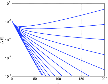
Figure 1: (Color online) Relative energy, $\Delta E_{\epsilon}(t)$, of the perturbed DW for 13 different values of the applied field $H_{1}$. See text for discussion.

Figure 1 shows the dependence of the relative energy $\Delta E_{\epsilon}$ on time $t$ for different values of the applied field $H_{1}$. The figure presents 13 curves corresponding, from top to bottom, to $H_{1}$ varying from $-1.2$ to $0$ at the increment of $0.1$. In the initial condition given by Eq. (60), we take $\epsilon_{1}=0.1$ and $\epsilon_{2}=\pi/50$.

Figure 1 clearly indicates that $\Delta E_{\epsilon}(t)$ decays exponentially for weak applied fields, $|H_{1}|\leq 1/2$, in accord with the analytic result Eq. (31). However, for $|H_{1}|\sim 1$, deviations from exponential decay are evident, and the precessing solution appears to become unstable for $|H_{1}|\gtrsim 1$.

V.2 Small hard-axis anisotropy

We consider next the evolution of a DW from an optimal profile at $t=0$ when the hard-axis anisotropy $K_{2}$ is nonvanishing. We fix $H_{1}=-0.5$.

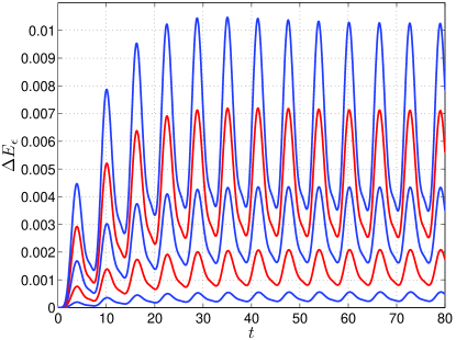
Figure 2: (Color online) Relative energy, $\Delta E_{\epsilon}(t)$, of the perturbed DW for 5 different values of the hard-axis anisotropy constant $K_{2}$. See text for discussion.

Figure 2 shows the dependence of the relative energy $\Delta E_{\epsilon}$ on time $t$ for different values of $K_{2}$. The figure presents 5 curves corresponding, from top to bottom, to $K_{2}$ varying from $0.1$ to $0.02$ at the decrement of $0.02$. (The blue and red colorings alternate to make adjacent curves more easily distinguishable.) It is evident that the relative energy remains small, verifying the linear analysis of Sec. III.

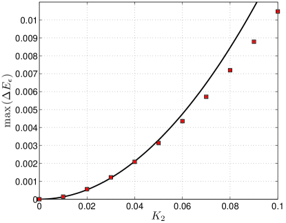
Figure 3: (Color online) Maximum value of the relative energy $\Delta E_{\epsilon}$ of the perturbed DW as a function of the hard-axis anisotropy $K_{2}$. Numerically computed values are represented by (red) squares. The (black) solid curve is a parabola, $\max(\Delta E_{\epsilon})=C_{K}K_{2}^{2}$ with $C_{K}=1.3207$, fitted by the method of least squares through the data points with $K_{2}\leq 0.04$.

Figure 3 shows the maximum value of the relative energy $\Delta E_{\epsilon}$ (over the interval $0\leq t\leq 80$) as a function of $K_{2}$. Red squares represent numerically computed values. The black solid curve is the parabola $C_{K}K_{2}^{2}$, with $C_{K}=1.3207$ fitted by the method of least squares through the data points with $K_{2}\leq 0.04$. We obtain convincing confirmation of the leading-order analytical result Eq. (48). For larger values of $K_{2}$, we see departures from quadratic dependence; for sufficiently large values of $K_{2}$ (not shown), the Walker solution was recovered.

V.3 Small transverse applied field

Finally, we address the stability of the precessing solution under an applied magnetic field, ${\bf H}_{a}=H_{1}\hat{{\bf x}}+H_{2}\hat{{\bf y}}$, with a small transverse component, $H_{2}(x)$. As discussed in Sec. IV, we want $H_{2}(x)$ to vanish as $x\rightarrow\pm\infty$. Here we take

$$H_{2}(x)={\bar{H}}_{2}w(x),$$ (61)

where $w(x)$ is equal to one inside the window $0\leq x\leq 20$ and vanishes outside (the argument of Section IV is easily modified to establish the linear stability result Eq. (48) in this case). We consider the evolution of a DW given at $t=0$ by the optimal profile $\mathbf{m_{*}}$ centred at $x=0$. We take $H_{1}=-0.5$, so that in the absence of the transverse field, the DW velocity is positive (cf. Eq. (13)) and the DW crosses the window. We take $K_{2}=0$.

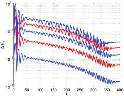
Figure 4: (Color online) Relative energy, $\Delta E_{\epsilon}(t)$, of the perturbed DW for 5 different values of the transverse field amplitude $\bar{H}_{2}$. See text for discussion.

Figure 4 shows the dependence of the relative energy $\Delta E_{\epsilon}$ on time $t$ for different values of the transverse field amplitude $\bar{H}_{2}$. The figure presents 5 curves corresponding, from top to bottom, to $\bar{H}_{2}$ varying from $0.1$ to $0.02$ at the decrement of $0.02$. (The blue and red colorings alternate to make adjacent curves more easily distinguishable.) The relative energy $\Delta E_{\epsilon}(t)$ is presented over the time interval $0\leq t\leq 400$, which, for small values of $\bar{H}_{2}$, is sufficient for the DW to traverse the spatial window $0\leq x\leq 20$ (cf. Eq. (13)). The results confirm that the relative energy of the perturbed magnetization profile remains small for small values of $\bar{H}_{2}$, in accord with the leading-order results of Section IV.

Figure 5: (Color online) Maximum value of the relative energy $\Delta E_{\epsilon}$ of the perturbed DW as a function of the amplitude of the transverse applied field, $\bar{H}_{2}$. Numerically computed values are represented by (red) squares. The (black) solid curve is a parabola, $\max(\Delta E_{\epsilon})=C_{H}\bar{H}_{2}^{2}$ with $C_{H}=99.6586$, fitted by the method of least squares through the data points with $\bar{H}_{2}\leq 0.04$.

Figure 5 shows the maximum value of the relative energy $\Delta E_{\epsilon}$ (over the interval $0\leq t\leq 400$) as a function of $\bar{H}_{2}$. Red squares represent numerically computed values. The black solid curve corresponds to the parabola $C_{H}\bar{H}_{2}^{2}$ with $C_{H}=99.6586$ fitted by the method of least squares through the data points with $\bar{H}_{2}\leq 0.04$. The figure provides a confirmation of the leading-order analytical result of Sec. IV that the maximum relative energy depends quadratically on $\bar{H}_{2}$ for small $\bar{H}_{2}$. Deviations from the parabolic dependence can be seen for $\bar{H}_{2}\gtrsim 0.08$.

VI Conclusions

The precessing solution is a new, recently reported exact solution of the Landau-Lifschitz-Gilbert equation. It describes the evolution of a magnetic domain wall in a one-dimensional wire with uniaxial anisotropy subject to a spatially uniform but time-varying applied magnetic field along the wire. We have analysed the stability of the precessing solution. We have proved linear stability with respect to small perturbations of the initial conditions as well as to small hard-axis anisotropy and small transverse applied fields, provided the applied magnetic field along the wire is not too large. We have also carried out numerical calculations that confirm full nonlinear stability under these perturbations.

Numerical calculations suggest that, for sufficiently large perturbations and applied longitudinal fields, the precessing solution becomes unstable, and new stable solutions appear. It would be interesting to analyse these bifurcations and study these new regimes for DW motion.