The Friedrichs Model and its use in resonance phenomena.

Abstract

We present here a relation of different types of Friedrichs models and their use in the description and comprehension of resonance phenomena. We first discuss the basic Friedrichs model and obtain its resonance in the case that this is simple or doubly degenerated. Next, we discuss the model with $N$ levels and show how the probability amplitude has an oscillatory behavior. Two generalizations of the Friedrichs model are suitable to introduce resonance behavior in quantum field theory. We also discuss a discrete version of the Friedrichs model and also a resonant interaction between two systems both with continuous spectrum. In an Appendix, we review the mathematics of rigged Hilbert spaces.

¹ Departamento de Física Teórica. Facultad de Ciencias, 47071 Valladolid, Spain.

² Institute for High Energy Physics, Protvino 142284, Moscow Region, Russia.

1 Introduction.

The Friedrichs model is a model aimed to describe the basic features of resonance phenomena. The basic idea is considering resonances associated to a Hamiltonian pair $\{H_{0},H\}$, where $H_{0}$ is the Hamiltonian for the “non perturbed” dynamics. $H_{0}$ has a simple non-degenerate absolutely continuous spectrum that coincides with the positive semiaxis. In addition, $H_{0}$ has at least an eigenvalue imbedded in the continuous spectrum. The total or “perturbed” Hamiltonian has the form $H=H_{0}+\lambda V$, where $V$ is a potential and $\lambda$ a coupling parameter that it is usually taken to be real (to preserve the self adjointness of $H$) and positive. The potential depends on a form factor function $f(\omega)$, which determines the existence and properties of the resonance. The action of the potential is to transform the bound state into a resonance, characterized by a point in the complex plane, as shall be described below. This point depends analytically on the coupling parameter $\lambda$. This is the basic description of the model as originally introduced by Friedrichs in 1948 [50].

The first step to show that the Fridrichs model is an excellent device in order to understand the machinery of decay in Quantum Mechanics accessible to physicists was given by Horwitz and Marchand [59]. After that, there were given several generalizations of the original model for various purposes including a description of unstable theory of fields.

In the present review, we intend to discuss most of the known versions of The Friedrichs model together their applications to model various situations in which quantum decay appears.

The Fridrichs model was conceived as mathematically rigorous and exactly solvable so that it could well serve as a toy model for a precise description of quantum decay. Also its possible generalizations are enormous in number and vast in applications. The present review is a first step to collect these generalizations. In order not to make this paper excessively long, we have selected some of these generalizations and not included a few ones. Our selection has been biased by our own work in the field. Examples of generalizations of the Fridrichs model that we have not included in our review are:

i.) The Fano-Anderson model [47, 2, 70]. This is a Fridrichs model in which the unperturbed Hamiltonian has a bounded absolutely continuous spectrum. This model is useful in solid state physics to analyze instabilities due to the presence of resonances (see references in [70]).

ii.) The Cascade model [37]. This is a model for unstable field theory.

iii.) A typical example of a generalization of the Fridrichs model that cannot be solved unless we make some rather severe approximations is given in a description of the boson-fermion interaction in nuclei developed by our group [39, 40].

We also do not intend to discuss some special physical features concerning to decay, such as the Zeno effect that deserves a whole monograph both by its extension and importance [72, 83]. Neither the possible relation of the Friedrichs model with a model for quantum systems with diagonal singularity [17, 18, 36].

We are mainly concern in the study of resonances in the Friedrichs model ant its various generalizations and we have obtained these resonances by means of the resolvent and not through the $S$ matrix. Consequently, we did not attempt to obtain in our examples the $S$ matrix or the Møller operators, which being relevant in a study of scattering are not necessary for our purposes.

The list of topics to be discussed in the present monograph goes as follows: In Section 2, we introduce a the basic Friedrichs model having a simple and as well as a double pole resonance. We define basic features in a language which can be accessible to both mathematicians and physicists. We devote 2.1, to the description of the resonance that emerges along the construction and properties of its corresponding Gamow vector, i.e., the state vector that decays exponentially. We also include a situation in which the resonance comes from a double pole of the resolvent. In this case, the exponential decay of the resonance is multiplied by a linear function of time.

The original Friedrichs model considers that the unperturbed Hamiltonian $H_{0}$ has one bound state only. What if we assume that $H_{0}$ has more than one bound states? Then, the solution to the problem becomes more complex. In Section 3, we consider the case in which $H_{0}$ has two bound states which become resonances due to the interaction with the potential. This is the two level Friedrichs model.

The study of the $N$ level Fridrichs model is of particular interest. Here, the decay behavior, given by the survival probability, although modulated by an exponential, becomes oscillatory. This fact has been observed experimentally [103], which incidentally shows the interest of these particular model in physics.

In Section 5, we introduce two generalizations of the Friedrichs model to describe resonances in relativistic quantum field theory. In the first case, two scalar relativistic quantum fields $\psi$ and $\varphi$ with respective masses $M$ and $m$ have an interaction of the type $\psi\varphi^{2}$. This problem can be solved on a sector in which a particle $\psi$ decays into two particles $\varphi$. The solution is provided by a generalization of the Friedrichs model, which shows resonances if $M>2m$ and can be exactly solved.

In the second case, we study the interaction between two boson fields. One is a local field and the other a bilocal field with a continuous bounded mass spectrum. The interaction between these two fields is quadratic. This situation can be solved by formulating it in terms of a generalized Friedrichs model that can be exactly solved due to the fact that the interaction in quadratic.

We conclude this section with a discussion of a Friedrichs model suitable for virtual transitions, which is possibly the simplest second quantization of the Friedrichs model. It studies the formation of a photon cloud around an atom.

In Section 6, we present a miscellaneous selection of Friedrichs models. The former is a discrete version. Here, the non-interaction hamiltonian is a harmonic oscillators plus a bath of harmonic oscillators. Then, an interaction is switched on between the first oscillator and the bath. The second one has the originality of producing an interaction between two Hamiltonians with continuous spectrum. One of these Hamiltonians, corresponding to an internal channel, has a bounded continuous spectrum doubly degenerated. The second one, corresponding to the external channel, has a continuous spectrum coinciding with the positive semiaxis and is infinitely degenerated. An interaction intertwines both Hamiltonians. As a consequence, the continuous spectrum of the Hamiltonian of the internal channel is transformed in a branch cut for the resolvent of the total Hamiltonian. This branch cut is interpreted as a type of generalized resonance similar to the one obtained in Yukawa type interactions [79].

We finish the paper with two Appendices. In the former, we discuss the concept and main properties of Rigged Hilbert Spaces (RHS). RHS are essential in the definition and presentation of properties of Gamow vectors, or vector states for resonances. In a second Appendix, we show how to calculate the reduced resolvent, which gives the localization of the resonances, for the basic Friedrichs model.

Although we are not going to study in depth the physical consequences of this model, a comment could be in order here. With respect to the relation between branch points and van Hove singularities, it has been reported [54] a behavior which is contrary to which is obtained in the basic Friedrichs model: for low dimensional systems the van Hove singularity leads to a non-analytic dependence on the decay rate associated with the resonance on the coupling constant.

Next, we start with the definition of resonance that we shall use in the sequel.

1.1 Definition of resonance: comments.

A resonance can be defined into several ways. It can be defined through the resolvent, or the behavior of the analytic continuation of the $S$-matrix. Both ways can be shown to be equivalent in specific models like the standard Friedrichs model.

Any definition of resonance in nonrelativistic Quantum Mechanics relies in the existence of two dynamics, a free dynamics, represented by the unperturbed or free Hamiltonian $H_{0}$ and a perturbed dynamics given by the total Hamiltonian $H=H_{0}+V$, where $V$ is a potential responsible of the resonance behavior. Both Hamiltonians are densely defined on an infinite dimensional Hilbert space $\cal H$ of pure states of the system under study.

After the properties of the resolvent of a self adjoint operator, we now that the resolvents

$$R_{H_{0}}(\psi,z):=\langle\psi|\frac{1}{H_{0}-zI}|\psi\rangle\hskip 28.45274ptR_{H}(\psi,z):=\langle\psi|\frac{1}{H-zI}|\psi\rangle$$ (1.1)

are analytic on the complex variable $z$ with a branch cut that coincides with the continuous spectrum of $H_{0}$ and $H$, that we usually assume to be equal, in both cases, to the positive semiaxis ${\mathbb{R}}^{+}$.

Next, we make the following assumptions:

i.) There is a dense set $\cal D$ of vectors in $\cal H$ such that both $R_{H_{0}}(\psi,z)$ and $R_{H}(\psi,z)$ admit an analytic continuation through the cut.

ii.) For some $\psi\in\cal D$, the partial resolvent $R_{H}(\psi,z)$ has an isolated singular point (in general a pole) at a point $z_{0}$ of analyticity of $R_{H_{0}}(\psi,z)$.

Then, we say that the Hamiltonian pair has a resonance at the point $z_{0}$ [89].

This is the definition that we shall use in the Friedrichs model. A second definition of resonance is also very much used and is suitable for the Friedrichs model:

Let us consider that the Hamiltonian pair $\{H_{0},H\}$ satisfies the sufficient conditions such that the $S$ operator exists. In this case, an incoming free state $\psi$ (evolving under the free dynamics $H_{0}$) will undergo the interaction given by the potential $V:=H-H_{0}$ and will be released as a free state $\varphi$. The relation between this incoming and outgoing free states is given by the $S$-operator in the form:

$$\varphi=S\psi$$

In the energy representation, we can write $\varphi(E)=S(E)\psi(E)$. Thus, the $S$-operator is a function of the energy $E$ (and eventually of other variables). In general, $S(E)$ is a complex analytic function with no other singularities than a branch cut coinciding with the positive semiaxis (and we assume that ${\mathbb{R}}^{+}$ is the continuous spectrum of both $H_{0}$ and $H$ [79, 23].

If the function of complex variable $S(z)$ determined by $S(E)$ has analytic continuation through the cut (and this can be shown to be the case under very general causality conditions [79]) and this continuation has poles outside the negative part of the real axis (then these poles come in complex conjugate pairs), then these poles are assumed to be resonance poles [23].

Thus, each resonance pole has a real part $E_{R}$ and a nonzero imaginary part $-i\Gamma/2$. The energy $E_{R}$ corresponds to the maximum of the bump of the cross section (whenever this equivalence applies) or the resonance energy and $\gamma$ is the width of this bump (related to the mean life of the resonance).

The relation between the latter definition of resonance and other definitions (bump in the cross section, sudden change in the phase shift, etc) is discussed in [23].

There are other definitions of resonances in quantum mechanics that appear in the literature. Under general conditions, these definitions are equivalent either to the resolvent or the $S$ matrix point of view. These are:

i.) Resonances are the eigenvalues of the dilated Hamiltonian. A dilation (or dilatation) is a transformation $U(\theta)$ on $L^{2}({\mathbb{R}}^{3})$ depending on a complex parameter $\theta$, defined as follows:

$$U(\theta)\psi({\bf x})=e^{3\theta/2}\,\psi(e^{\theta}{\bf x})\,.$$

Clearly if $\theta$ is real, $U(\theta)$ is unitary. Dilations are used to define a large class of nonlocal potentials called dilation analytic potentials [88]. If $V$ is a dilation analytic potential, then define:

$$H(\theta):=U(\theta)[H_{0}+V]U^{-1}(\theta)=e^{-2\theta}\,H_{0}+V(\theta)\,.$$

Then, resonances are the solutions of the eigenvalue equation:

$$H(\theta)\psi_{R}(\theta)=z_{R}\psi_{R}(\theta)\,.$$

The value of the eigenvalue $z_{R}$ of $H(\theta)$ does not depend on the parameter $\theta$ and these eigenvalues are resonances according to the definition which makes use of the partial resolvent. For details, see [88]. Dilatations really provide a method to obtain resonances called the complex scaling method.

ii.) When the potential is spherically symmetric, one form of finding resonances is obtaining solutions of the Schrödinger equation with complex eigenvalues, $\chi(r,z_{0})$ satisfying the so called purely outgoing boundary conditions. This means that as $k\longmapsto\infty$, then $\chi(r,z_{0})\sim e^{ikr}$, i.e., only outgoing wave function can exists. These complex eigenvalues $z_{0}$ can be identified with resonances and are poles of the $S$ matrix.

iii.) Resonances are also defined as complex eigenvalues of a dissipative operator in the context of the Lax-Phillips formalism. This can be found in [94, 93, 84].

There are relations between these definitions of resonances. As was mentioned above, some of them are consequences of others. For a review in this subject, see [4] and references thereof.

2 The standard Friedrichs model.

We shall present in here the Friedrichs model in its most simple form, which has been described in many places [50, 59, 15, 13, 38, 7, 95, 96, 85, 81]. We can introduced it in two different languages: Hilbert space language or bra ket formalism. The latter makes use of the rigged Hilbert space construction that we describe in the last part of the present review. Although we shall use of the bra-ket formalism along our presentation, we discuss briefly the Hilbert space presentation first and then we shall go to the second one which is more familiar to most users. Then, in its simplest basic form, the Friedrichs model includes the following ingredients:

1.- A (infinite dimensional) Hilbert space $\cal H$. If we use the energy representation, this Hilbert space is given by:

$${\cal H}:={\mathbb{C}}\oplus L^{2}({\mathbb{R}}^{+})\,.$$ (2.1)

Here, $\mathbb{C}$ is the field of complex numbers, ${\mathbb{R}}^{+}$ is the positive semiaxis ${\mathbb{R}}^{+}=[0,\infty)$ and $L^{2}({\mathbb{R}}^{+})$ is the Hilbert space of square integrable functions on ${\mathbb{R}}^{+}$. We say that we are using the energy representation because the Hamiltonians we shall use in this Friedrichs model will have a continuous spectrum coinciding with ${\mathbb{R}}^{+}$, then the space of the wave functions in the energy representation is then $L^{2}({\mathbb{R}}^{+})$.

After (2.1), any $\psi\in\cal H$ can be written in matricial form as:

$$\psi=\left(\begin{array}[]{c}\alpha\\[8.61108pt] \varphi(\omega)\end{array}\right)\,,$$ (2.2)

where $\alpha$ is an arbitrary complex number and $\varphi(\omega)$ an arbitrary function in $L^{2}({\mathbb{R}}^{+})$. The scalar product of two vectors in $\cal H$ is given by

$$\left(\left(\begin{array}[]{c}\alpha\\[8.61108pt] \varphi(\omega)\end{array}\right),\left(\begin{array}[]{c}\beta\\[8.61108pt] \eta(\omega)\end{array}\right)\right)=\alpha^{*}\beta+\int_{0}^{\infty}\varphi^{*}(\omega)\eta(\omega)\,d\omega\,.$$ (2.3)

Here, $\beta$ is a complex number and $\eta(\omega)\in L^{2}({\mathbb{R}}^{+})$.

2.- In order to create resonance phenomena, we need a pair of Hamiltonians: a free Hamiltonian $H_{0}$ and a total or perturbed Hamiltonian $H$, such that the pair $\{H_{0},H\}$ is able to create resonances. We here construct such a pair. Let us begin with $H_{0}$. Its domain (the subspace of all vectors $\psi\in\cal H$ such that $H_{0}\psi\in\cal H$) is given by the vectors in the form (2.2) such that $\omega\varphi(\omega)\in L^{2}({\mathbb{R}}^{+})$. The action of $H_{0}$ on a vector in its domain is given by

$$H_{0}\left(\begin{array}[]{c}\alpha\\[8.61108pt] \varphi(\omega)\end{array}\right)=\left(\begin{array}[]{c}\omega_{0}\alpha\\[8.61108pt] \omega\varphi(\omega)\end{array}\right)\,,$$ (2.4)

where $\omega_{0}$ is a real positive number, i.e., $\omega_{0}>0$. Observe that the vector

$$|1\rangle=\left(\begin{array}[]{c}1\\[8.61108pt] 0\end{array}\right)$$ (2.5)

is an eigenvector of $H_{0}$ with eigenvalue $\omega_{0}$, i.e., $H_{0}|1\rangle=\omega_{0}|1\rangle$. Note that

$$H_{0}\left(\begin{array}[]{c}0\\[8.61108pt] \varphi(\omega)\end{array}\right)=\left(\begin{array}[]{c}0\\[8.61108pt] \omega\varphi(\omega)\end{array}\right)\,,$$ (2.6)

which means that $H_{0}$ is the multiplication operator, for the second component, on the interval ${\mathbb{R}}^{+}=[0,\infty)$. We conclude that, by construction, $H_{0}$ has a non degenerate absolutely continuous spectrum that coincides with $[0,\infty)$, plus an eigenvalue, $\omega_{0}$. Since $\omega_{0}>0$, this unique eigenvalue of $H_{0}$ is embedded in the continuous spectrum of $H_{0}$.

3.- The total Hamiltonian has the form $H=H_{0}+\lambda V$, where $\lambda$ is a coupling constant and $V$ is a potential to be defined. In order to create resonances, $V$ should produce an interaction between discrete and continuous parts of $H_{0}$. It is proposed in the form:

$$V\psi=\left(\begin{array}[]{c}\int_{0}^{\infty}f(\omega)\varphi(\omega)\,d\omega\\[8.61108pt] \alpha f^{*}(\omega)\end{array}\right)\,,$$ (2.7)

where $\psi$ is the arbitrary vector of $\cal H$ given by (2.1) and $f(\omega)$ is a function on ${\mathbb{R}}^{+}$ called the form factor. Observe that $V\psi\in\cal H$ for each $\psi\in\cal H$ if and only if $f(\omega)\in L^{2}({\mathbb{R}}^{+})$. If this were the case, the domain of $V$ is $\cal H$ (and $V$ is bounded!) and the domain of $H$ coincides with the domain of $H_{0}$. This may suggest that we cannot allow for $f(\omega)$ outside $L^{2}({\mathbb{R}}^{+})$. The total Hamiltonian $H$ has a continuous nondegenerate spectrum equal to $[0,\infty)$.

So far, we have introduced the basic features of the Friedrichs model, without a discussion of its properties. Let us translate the above definition in terms of the bra-ket formalism.

We have already defined the ket $|1\rangle\in\cal H$. For each $\omega$ in the (absolutely) continuous spectrum of $H_{0}$, there is an (generalized) eigenvector of $H_{0}$, $|\omega\rangle$, with eigenvalue $\omega$, i.e., $H_{0}|\omega\rangle=\omega|\omega\rangle$. Taking this into account, we can use the following notation for an arbitrary vector $\psi$ as in (2.2):

$$\psi=\alpha|1\rangle+\int_{0}^{\infty}\varphi(\omega)|\omega\rangle\,d\omega\,.$$ (2.8)

The expression for the free Hamiltonian can be derived from the spectral representation theorem [86] (see the specific form to translate integral spectral representations into the bra-ket formalism in [10] and a generalization in [52]). In our case, it takes the following form:

$$H_{0}=\omega_{0}|1\rangle\langle 1|+\int_{0}^{\infty}\omega\,|\omega\rangle\langle\omega|\,d\omega\,,$$ (2.9)

where $|1\rangle\langle 1|$ is the projection into the bound state $|1\rangle$ of $H_{0}$ and $|\omega\rangle\langle\omega|$ a similar object that can be defined for $|\omega\rangle$.

Apart from the coupling constant $\lambda$, the interaction potential $V$ can be written in the following form:

$$V=\int_{0}^{\infty}[f(\omega)\,|\omega\rangle\langle 1|+f^{*}(\omega)|1\rangle\langle\omega|\,]\,d\omega\,,$$ (2.10)

where $f(\omega)$ is the form factor that determines the behavior of the interaction. We recall that the form factor should be kept square integrable on the positive semiaxis if we want to keep the model in the context of Hilbert space, although this restriction may be unnecessary. Also, the form factor could be real or complex, it does not matter. From (2.9), we clearly see that $V$ produces an interaction between the continuous and discrete parts of $H_{0}$ modelled by the form factor function. We want to repeat again that the interaction also depends on the form factor $\lambda$, so that $H=H_{0}+\lambda V$.

We want to show that even this simple Friedrichs model shows resonance behavior. In fact, this resonance is produced when the action of the interaction “dissolves” the discrete spectrum of $H_{0}$ in the continuum. This process depends crucially of the form factor $f(\omega)$. The position of the resonance will also depend on the coupling constant $\lambda$ [44].

In order to search for resonance behavior, we need to fix a definition of resonance and we shall use the definition proposed in [88] that we have presented earlier (see (1.1)). Accordingly, let us consider the projection $P:=|1\rangle\langle 1|$ into the subspace spanned by the eigenvector $|1\rangle$ of $H_{0}$. Pick $\psi\in\cal H$, as in (2.8). Then, $P\psi=\alpha|1\rangle$. Then, take the operator, called the reduced resolvent:

$$P(H-zI)^{-1}P\,,$$ (2.11)

where $I$ is the identity operator. Then, consider the function on the complex variable $z$, depending of the vector $\psi\in\cal H$:

$$R_{\psi}(z):=\langle\psi|P(H-zI)^{-1}P|\psi\rangle=|\alpha|^{2}\,\langle 1|\frac{1}{H-zI}|1\rangle\,.$$ (2.12)

The real number $|\alpha|^{2}$ is irrelevant in the discussion of the analytic properties of $R_{\psi}(z)$, which are only contained in the following function independent of $\psi$:

$$\frac{1}{\eta(z)}:=\langle 1|\frac{1}{H-zI}|1\rangle\,.$$ (2.13)

If this function, has an analytic continuation and the continuation has an isolated pole at $z_{0}=E_{R}-i\Gamma/2$ with nonzero imaginary part, this pole should be associated to a resonance, according to the definition of resonances from the resolvent properties [88]. The real part of $z_{0}$, $E_{R}$ is the resonance energy (or location of the maximum of the bump of the cross section) and $\Gamma$ the width of the bump.

By extension, (2.13) is also called the reduced resolvent.

Some sufficient conditions for this analytic continuation to exist and have the desired properties have been studied in [59, 44]. These are conditions on the form factor $|f(\omega)|^{2}$. Under these conditions, we can find an explicit expression for $\eta(z)$ in (2.3) [44]:

$$\eta(z)=z-\omega_{0}-\lambda^{2}\int_{0}^{\infty}\frac{|f(\omega)|^{2}}{z-\omega}\,d\omega\,.$$ (2.14)

Under the sufficient conditions mentioned earlier [44], $\eta(z)$ is an analytic function on the complex plane $\mathbb{C}$ with a cut coinciding with the positive semiaxis (the continuous spectrum of both $H_{0}$ and $H$) and admits analytic continuations beyond the cut from above to below and from below to above. In the first case, the boundary values of the function on the positive semiaxis are given by:

$$\eta_{+}(x)=x-\omega_{0}-\lambda^{2}\int_{0}^{\infty}\frac{|f(\omega)|^{2}}{x-\omega+i0}\,d\omega$$ (2.15)

and in the second:

$$\eta_{-}(x)=x-\omega_{0}-\lambda^{2}\int_{0}^{\infty}\frac{|f(\omega)|^{2}}{x-\omega-i0}\,d\omega\,.$$ (2.16)

These analytic continuations have respective zeroes at the points $z_{0}=E_{R}-i\Gamma/2$ and its complex conjugate $z_{0}^{*}=E_{R}+i\Gamma/2$ (observe that (2.15) and (2.16) are complex conjugate of each other), under the mentioned sufficient conditions [44]. Correspondingly, the analytic continuation of the inverses $\eta_{+}^{-1}(x)$ and $\eta_{-}^{-1}(x)$ have poles at $z_{0}$ and $z_{0}^{*}$ respectively.

It is important to remark that the meaning of the kets $|\omega\rangle$, some of the above formulas like (2.8-2.10) as well as the Gamow vectors that will be introduced from the next section onwards, have a meaning in the context of extensions of Hilbert space called rigged Hilbert spaces. We shall add in the appendices a discussion on this mathematical tools and their applications in the theory of resonances.

2.1 Simple pole resonances.

These resonance poles may be simple or multiple. The case of the Friedrichs model with simple pole resonances is the easiest to study, yet containing all the nontrivial information concerning resonance behavior. As we have seen before, these resonance poles come into complex conjugate pairs.

The next objective is to find the Gamow vector for this resonance. With this goal, let us construct the general state vector in the following form:

$$\psi=\alpha\,|1\rangle+\int_{0}^{\infty}\varphi(\omega)\,|\omega\rangle\,d\omega\,.$$ (2.17)

We want to emphasize that discrete and continuous degrees of freedom are orthogonal. This idea implies the following relations:

$$\langle 1|1\rangle=1\,,\hskip 11.38092pt\langle 1|\omega\rangle=\langle\omega|1\rangle=0\,,\hskip 11.38092pt\langle\omega|\omega^{\prime}\rangle=\delta(\omega-\omega^{\prime})\,.$$ (2.18)

The Gamow vectors are defined as the generalized eigenvectors of the total Hamiltonian with complex eigenvalues. These eigenvalues coincide with the resonance poles (as poles of the analytic continuation of the resolvent). As resonance poles come into complex conjugate pairs (in the energy representation), let us denote by $z_{0}$ and $z^{*}_{0}$ the poles corresponding to a given resonance. Then, their corresponding eigenvectors (Gamow vectors) are denoted by $|f_{0}\rangle$, $|\tilde{f}_{0}\rangle$, so that

$$H\,|f_{0}\rangle=z_{0}\,|f_{0}\rangle\,;\hskip 19.91684ptH\,|\tilde{f}_{0}\rangle=z_{0}^{*}|\tilde{f}_{0}\rangle\,.$$ (2.19)

Thus, in order to obtain the Gamow vectors, we have to solve the above equations. The technique is the following: Let us write the eigenvalue equation for all $x\geq 0$:

$$(H-x)\Psi(x)=0\,.$$ (2.20)

Here $\Psi(x)$ is the (generalized) eigenvector of $H$ with eigenvalue $x$. The set of eigenvectors $\Psi(x)$ can be written in the following form:

$$\Psi(x)=\alpha(x)\,|1\rangle+\int_{0}^{\infty}\varphi(x,\omega)\,|\omega\rangle\,d\omega\,,$$ (2.21)

for all $x>0$.

The next step is to carry (2.21) into (2.20). The result is:

$$(H-x)\Psi(x)=(\omega_{0}-x)\alpha(x)\,|1\rangle+\lambda\int_{0}^{\infty}f^{*}(\omega)\varphi(x,\omega)\,d\omega\,\,|1\rangle$$

$$+\int_{0}^{\infty}(\omega-x)\varphi(x,\omega)\,|\omega\rangle\,d\omega+\lambda\alpha(x)\int_{0}^{\infty}f(\omega)\,|\omega\rangle\,d\omega=0\,.$$ (2.22)

Taking into account that the bound state $|1\rangle$ and the continuum are linearly independent, since they are orthogonal degrees of freedom (see relations (2.18)) and omitting the vectors $|1\rangle$ in the first equation and $|\omega\rangle$ in the second, relation (2.22) becomes the following pair of equations:

$$(\omega_{0}-x)\,\alpha(x)+\lambda\int_{0}^{\infty}\varphi(x,\omega)\,f^{*}(\omega)\,d\omega=0$$ (2.23)

$$(\omega-x)\varphi(x,\omega)+\lambda\alpha(x)\,f(\omega)=0\,.$$ (2.24)

Equation (2.24) can be written as:

$$\varphi(x,\omega)=\lambda\frac{\alpha(x)f(\omega)}{x-\omega\pm i0}+c\delta(x-\omega)\,,$$ (2.25)

where $c$ is an arbitrary constant that can be chosen equal to one ($c=1$), without any change in the essential results. We see that two solutions appear, one for each continuation (from above to below and from below to above). Then, equation (2.25) becomes

$$(\omega_{0}-x)\alpha(x)+\lambda^{2}\alpha(x)\int_{0}^{\infty}\frac{|f(\omega)|^{2}}{x-\omega\pm i0}\,d\omega+\lambda f^{*}(x)=0\,.$$ (2.26)

If we denote as

$$\eta_{\pm}(x):=\omega_{0}-x+\lambda^{2}\int_{0}^{\infty}\frac{|f(\omega)|^{2}}{x-\omega\pm i0}\,d\omega\,,$$ (2.27)

equation (2.26) yields

$$\alpha(x)=-\lambda\frac{f^{*}(x)}{\eta_{\pm}(x)}\,.$$ (2.28)

If we carry this results into (2.22), we finally obtain:

$$\Psi_{\pm}(x)=|x\rangle-\frac{\lambda f^{*}(x)}{\eta_{\pm}(x)}\left[|1\rangle+\lambda\int_{0}^{\infty}\frac{f(\omega)}{x-\omega\pm i0}\,|\omega\rangle\,d\omega\right]\,.$$ (2.29)

Let us take one of these two vectors, say $\Psi_{+}(x)$. This vector is a functional on a certain space of test vectors, ${\bf\Phi}_{+}$ as we shall discuss in the Appendix. When we apply $\Psi_{+}(x)$ to a test vector $\varphi_{+}\in{\bf\Phi}_{+}$, the result gives a function on the variable $x$, $\langle\Psi_{+}(x)|\varphi_{+}\rangle$ which admits an analytic continuation on the lower half plane, $\langle\Psi_{+}(z)|\varphi_{+}\rangle$. This continuation has a pole at the point $z_{0}$, which is the zero of the function $\eta_{+}(z)$. We assume that this pole is simple. Sufficient conditions for this kind of situations exists and are discussed in [44]. Then, if we omit the arbitrary $\varphi_{+}\in{\bf\Phi}_{+}$, we can write on a neighborhood of $z_{0}$:

$$\Psi_{+}(z)=\frac{C}{z-z_{0}}+o(z)\,,$$ (2.30)

where $o(z)$ denotes a Taylor series on $z_{0}$, which converges on a neighborhood of $z_{0}$ (both $C$ and $o(z)$ are functionals on ${\bf\Phi}_{+}$).

Let us go back to (2.6). As the analytic continuation $\Psi_{+}(z)$ exists, the eigenvalue formula (2.6) should be also valid for any $z$ at which $\Psi_{+}(z)$ makes sense, so that we can write

$$(H-z)\Psi_{+}(z)=0\,.$$ (2.31)

Now, if we carry (2.30) into (2.31), we get:

$$0=(H-z)\Psi_{+}(z)=\frac{1}{z-z_{0}}\,(H-z)\,C+(H-z)\,o(z)\,,$$ (2.32)

which gives

$$(H-z_{0})\,C=0\Longrightarrow HC=z_{0}C\,.$$ (2.33)

This shows that the residue $C$ in (2.30) is precisely the Gamow vector corresponding to the resonance pole $z_{0}$. In order to obtain the explicit form for this Gamow vector, we just proceed as one does in a standard calculus of residua. As the pole comes from a zero of $\eta_{+}(z)\approx{\rm constant}(z-z_{0})+o(z)$, on a neighborhood of $z_{0}$, we have:

$$\Psi_{+}(z)\approx\frac{\rm constant}{(z-z_{0})}\;\left[|1\rangle+\lambda\int_{0}^{\infty}\frac{f(\omega)}{z-\omega+i0}\,|\omega\rangle\,d\omega\right]+o(z)\,.$$ (2.34)

Since [55]

$$\frac{1}{z-\omega+i0}=\frac{1}{z_{0}-\omega+i0}-\frac{z-z_{0}}{(z_{0}-\omega+i0)^{2}}+o(z)\,,$$ (2.35)

we have that

$$\Psi_{+}(z)\approx\frac{\rm constant}{(z-z_{0})}\;\left[|1\rangle+\lambda\int_{0}^{\infty}\frac{f(\omega)}{z_{0}-\omega+i0}\,|\omega\rangle\,d\omega\right]+o(z)\,.$$ (2.36)

Therefore, save for an irrelevant constant, we conclude that

$$C\equiv|f_{0}\rangle=|1\rangle+\int_{0}^{\infty}\frac{\lambda f(\omega)}{z_{0}-\omega+i0}\,|\omega\rangle\,d\omega\,.$$ (2.37)

With the vector $\Psi_{-}(x)$ as in (2.29), we can proceed analogously, now taking into account that the function $\eta_{-}(x)$ has a simple pole at $z_{0}^{*}$, the complex conjugate of $z_{0}$. By repeating the same arguments, we can obtain the solution $|\widetilde{f}_{0}\rangle$ of the eigenvalue equation $H|\widetilde{f}_{0}\rangle=z_{0}^{*}|\widetilde{f}_{0}\rangle$ as:

$$|\widetilde{f}_{0}\rangle=|1\rangle+\int_{0}^{\infty}\frac{\lambda f^{*}(\omega)}{z_{0}^{*}-\omega-i0}\,|\omega\rangle\,d\omega\,.$$ (2.38)

So far the discussion of the simplest Friedrichs model. The presentation of the model with a double pole resonance comes next.

2.2 Double pole resonances.

In order to show that there exists a Friedrichs model allowing for double pole resonances, we have to construct an explicit form factor that produces this effect. From all the above discussions, we need to show that a given form factor produces a double zero for $\eta_{\pm}(z)$. Let us choose $f(\omega)$ such that

$$|f(\omega)|^{2}=\frac{\sqrt{\omega}}{P(\omega)}\,,$$ (2.39)

with

$$P(\omega):=(\omega-\beta)(\omega-\beta^{*})\,,$$ (2.40)

where $\beta$ is a complex number (with nonvanishing imaginary part!). With this choice, we obtain the following expression for the function $\eta(z)$, defined as in (2.13,2.14):

$$\eta(z)=\omega_{0}-z-\pi\lambda^{2}\left\{\frac{\sqrt{-z}}{P(z)}-\frac{1}{\beta-\beta^{*}}\left(\frac{\sqrt{-\beta}}{z-\beta}-\frac{\sqrt{-\beta^{*}}}{z-\beta^{*}}\right)\right\}\,.$$ (2.41)

Next, we propose a change of variables which moves our formulas from the energy representation to the momentum representation:

$$z=p^{2}\hskip 17.07182pt;\hskip 17.07182pt\beta=b^{2}$$ (2.42)

and write $\varphi(p)=\eta(p^{2})=\eta(z)$. Obviously, $p$ is a complex variable. We have that

$$\varphi(p)=\omega_{0}-p^{2}+\frac{i\pi\lambda^{2}}{(b-b^{*})(p+b)(p-b^{*})}\,.$$ (2.43)

We shall show later that $\eta(z)$ has a double zero if and only if $\varphi(p)$ has a double zero. This is the first idea to be considered in order to determine under which conditions our model can have a double pole resonance. In addition, we have to fix certain constants. First of all, we have the complex constant $b$. This gives two undetermined real constants. But we can also play with the real constants $\omega_{0}$, $\lambda$ and with the real and imaginary parts of $p_{0}$, the double zero of $\varphi(p)$. Should $\varphi(p)$ have a double zero at the point $p_{0}$, it might fulfill the following conditions:

$$\varphi(p_{0})=0\hskip 14.22636pt;\hskip 14.22636pt\varphi^{\prime}(p_{0})=0\hskip 14.22636pt;\hskip 14.22636pt\varphi^{\prime\prime}(p_{0})\neq 0\,,$$ (2.44)

which give four equations, given by the real and imaginary components of the two identities in (2.44), and a relation for the six parameters mentioned in the previous paragraph: $\omega_{0},\lambda,{\rm Real}\,p_{0},{\rm Im}\,p_{0},{\rm Real}\,b$ and ${\rm Im}\,b$. Taking into account that we have two equations and six parameters, we have in principle two free parameters that can be chosen arbitrarily among these six. It seems natural to choose the real constants $\omega_{0}$ and $\lambda$ as free, since they are usually data in the Friedrichs model. Then, after not complicated algebraic manipulations, we have

$$b=\omega_{0}^{1/2}+2i\left(\frac{\pi\lambda^{2}}{16\omega_{0}}\right)^{1/3}\,,$$ (2.45)

$$p_{0}=\left[\omega_{0}-\left(\frac{\pi\lambda^{2}}{16\omega_{0}}\right)^{2/3}\right]-i\left(\frac{\pi\lambda^{2}}{16\omega_{0}}\right)^{1/3}\,.$$ (2.46)

If we carry (2.45) and (2.46) into (2.43), we obtain

$$\varphi(p)=-\frac{(p-p_{0})^{2}\,(p+p_{0}^{*})^{2}}{(p+\tau)\,(p-\tau^{*})}\,,$$ (2.47)

where $\tau$ is some complex number different from $p_{0}^{*}$, which is irrelevant in our discussion because it corresponds to a simple zero of the reduced resolvent. Equation (2.47) shows that $\varphi(p)$ has a double zero at the point $p_{0}$ and another double zero at its complex conjugate $p_{0}^{*}$.

Now, we have to show that the zeroes of $\eta(z)$ and $\varphi(p)$ coincide, after the change of variables, as well as their multiplicity. To begin with, let us assume that $\eta(z)$ has a double zero at $z_{0}$. Then, there exists a function $\chi(z)$ analytic on a neighborhood of $z_{0}$, with $\chi(z_{0})\neq 0$, and such that on this neighborhood one has:

$$\eta(z)=(z-z_{0})^{2}\chi(z)\,.$$

The function $\varphi(p)=\eta(p^{2})$ and therefore,

$$\varphi(p)=\eta(p^{2})=(p^{2}-p_{0}^{2})^{2}\chi(p^{2})=(p-p_{0})^{2}(p+p_{0})^{2}\chi(p^{2})\,.$$

If $\Delta(p):=(p+p_{0})^{2}\chi(p^{2})$, we have that $\Delta(p_{0})=2p_{0}^{2}\chi(p_{0}^{2})\neq 0$ and

$$\varphi(p)=(p-p_{0})^{2}\Delta(p)$$

and $\varphi(p)$ has a double pole at $p_{0}=\sqrt{z_{0}}$. Conversely, let us assume that $\varphi(p)$ has a double pole at $p_{0}$. Then, there exists an analytic function $\xi(p)$ on a neighborhood of $p_{0}$, with $\xi(p_{0})\neq 0$, such that

$$\varphi(p)=(p-p_{0})^{2}\xi(p)=\eta(z)\,.$$

Then, $\eta(z)$ has a double pole at $z_{0}=p_{0}^{2}$ if and only if the function $\frac{\eta(z)}{(z-z_{0})^{2}}$ has a nonvanishing limit if $z$ goes to $z_{0}$. Thus,

$$\lim_{z\mapsto z_{0}}\frac{\eta(z)}{(z-z_{0})^{2}}=\lim_{p\mapsto p_{0}}\frac{(p-p_{0})^{2}\xi(p)}{(p^{2}-p_{0}^{2})^{2}}=\lim_{p\mapsto p_{0}}\frac{(p-p_{0})^{2}\xi(p)}{(p-p_{0})^{2}(p+p_{0})^{2}}=\frac{\xi(p_{0})}{2p_{0}}\neq 0\,,$$

which proves our claim. The conclusion is that $\eta(z_{0})$ has a double zero at $z_{0}$ if and only if $\varphi(p)$ has a double zero at $p_{0}$ with $z_{0}=p_{0}^{2}$.

Consequently, the analytic continuation through ${\mathbb{R}}^{+}$ of (2.10) has a double pole at the points $z_{0}$ and $z_{0}^{*}$ and therefore the version of the Friedrichs model here discussed shows a double pole resonance.

We would like to obtain the Gamow vectors for this resonance. Once we have established the existence of a double pole resonance, on a neighborhood of $z_{0}$, the vector $\Psi_{+}(z)$ as in (2.29) has the following behavior:

$$\Psi_{+}(z)=\frac{C_{1}}{(z-z_{0})^{2}}+\frac{C_{2}}{z-z_{0}}+o(z)\,.$$ (2.48)

As in the case of a simple pole resonance, we have on a neighborhood of $z_{0}$

$$\Psi_{+}(z) \approx \frac{{\rm constant}}{(z-z_{0})^{2}}\left\{|1\rangle+\lambda\int_{0}^{\infty}\frac{f(\omega)}{z-\omega+i0}\,|\omega\rangle\,d\omega\right\}$$ (2.49)

$$= \frac{{\rm constant}}{(z-z_{0})^{2}}\left\{|1\rangle+\lambda\int_{0}^{\infty}\frac{f(\omega)}{z_{0}-\omega+i0}\,|\omega\rangle\,d\omega\right.$$

$$- \left.\lambda(z-z_{0})\int_{0}^{\infty}\frac{f(\omega)}{(z_{0}-\omega+i0)^{2}}\,|\omega\rangle\,d\omega\right\}\,.$$

Then,

$$C_{1} = |1\rangle+\lambda\int_{0}^{\infty}\frac{f(\omega)}{z_{0}-\omega+i0}\,|\omega\rangle\,d\omega$$ (2.50)

$$C_{2} = -\lambda\int_{0}^{\infty}\frac{f(\omega)}{(z_{0}-\omega+i0)^{2}}\,|\omega\rangle\,d\omega\,.$$ (2.51)

Now, taking into account (2.34), we have:

$$(H-z)\left[\frac{C_{1}}{(z-z_{0})^{2}}+\frac{C_{2}}{z-z_{0}}+o(z)\right]=0\,.$$ (2.52)

If we multiply (2.52) by $(z-z_{0})^{2}$ and take the limit as $z_{0}\longmapsto 0$, we obtain:

$$(H-z_{0})\,C_{1}=0\Longleftrightarrow HC_{1}=z_{0}C_{1}\,,$$ (2.53)

since $o(z)$ is a regular function on $z$. If now, we multiply (2.49) by $z-z_{0}$, we get

$$(H-z)\left[\frac{C_{1}}{z-z_{0}}+C_{2}+(z-z_{0})o(z)\right]=0$$

$$\Longrightarrow\frac{z_{0}-z}{z-z_{0}}C_{1}+(H-z)C_{2}+(z-z_{0})(H-z)o(z)=0\,.$$ (2.54)

Taking the limit as $z\longmapsto z_{0}$ in (2.54), one readily obtains

$$HC_{2}=z_{0}C_{2}+C_{1}\,.$$ (2.55)

Summarizing, we obtain the following relations

$$HC_{1}=z_{0}C_{1}\hskip 17.07182pt{\rm and}\hskip 17.07182ptHC_{2}=z_{0}C_{2}+C_{1}\,.$$ (2.56)

The vectors $C_{1}$ and $C_{2}$ are linearly independent (otherwise $C_{2}$ would be an eigenvector of $H$ with eigenvalue $z_{0}$ in clear contradiction of (2.55). These vectors belong to the antidual ${\bf\Phi}_{+}^{\times}$ in the rigged Hilbert space ${\bf\Phi}_{+}\subset{\cal H}\subset{\bf\Phi}_{+}^{\times}$ (see Appendix), thus, $C_{1}$ and $C_{2}$ are functionals. The restriction of $H$ on the two dimensional subspace of ${\bf\Phi}_{+}^{\times}$ with basis $\{C_{1},C_{2}\}$ has the following form

$$\left(\begin{array}[]{cc}z_{0}&1\\ 0&z_{0}\\ \end{array}\right)\,,$$ (2.57)

which shows a block diagonal form. This kind of structure has been discussed in several contexts in [33, 34, 73, 74, 75]. Conventionally, $C_{1}$ and $C_{2}$ are called $|f_{0}\rangle$ and $|f_{1}\rangle$ respectively [8, 38].

As with the Friedrichs model with a simple pole resonance, we can proceed analogously with the vector $\Psi_{-}(x)$ as in (2.26), now taking into account that the function $\eta_{-}(x)$ has a double pole at $z_{0}^{*}$, the complex conjugate of $z_{0}$. By repeating the same arguments, we can obtain the solution $|\widetilde{f}_{0}\rangle$ of the eigenvalue equation $H|\widetilde{f}_{0}\rangle=z_{0}^{*}|\widetilde{f}_{0}\rangle$ as in (2.38) and a second vector $|\widetilde{f}_{1}\rangle$, which is given by:

$$|\widetilde{f}_{1}\rangle=-\lambda\int_{0}^{\infty}\frac{f^{*}(\omega)}{(z_{0}^{*}-\omega-i0)^{2}}\,|\omega\rangle\,d\omega\,.$$ (2.58)

The vectors $|\widetilde{f}_{0}\rangle$ and $|\widetilde{f}_{1}\rangle$ belong to the antidual ${\bf\Phi}_{-}^{\times}$ of a rigged Hilbert space ${\bf\Phi}_{-}\subset{\cal H}\subset{\bf\Phi}_{-}^{\times}$ and are therefore functionals on the space ${\bf\Phi}_{-}$ to be defined in the appendix. As in the previous case, the total Hamiltonian $H$ can be extended into the antidual ${\bf\Phi}_{-}^{\times}$ and we can also prove the follwoing relations:

$$H|\widetilde{f}_{0}\rangle=z_{0}^{*}|\widetilde{f}_{0}\rangle\hskip 14.22636pt;\hskip 14.22636ptH|\widetilde{f}_{1}\rangle=z_{0}|\widetilde{f}_{1}\rangle+|\widetilde{f}_{0}\rangle\,.$$ (2.59)

Therefore, on the subspace spanned by the vectors $|\widetilde{f}_{0}\rangle$ and $|\widetilde{f}_{1}\rangle$ the total Hamiltonian has the following form:

$$H=\left(\begin{array}[]{cc}z_{0}^{*}&1\\ 0&z_{0}^{*}\\ \end{array}\right)\,.$$ (2.60)

We may also study the time evolution of the Gamow vectors $|f_{0}\rangle$, $|f_{1}\rangle$, $|\widetilde{f}_{0}\rangle$ and $|\widetilde{f}_{1}\rangle$ (sometimes also called Jordan-Gamow vectors, see [30]). As $|f_{0}\rangle$ and $|f_{1}\rangle$ in one side and $|\widetilde{f}_{0}\rangle$ and $|\widetilde{f}_{1}\rangle$ on the other belong to different spaces, we must study their time evolution separately. A thoroughly discussion has been presented elsewhere [8, 38]. The final result is given by

$$e^{-itH}|f_{0}\rangle = e^{-itz_{0}}|f_{0}\rangle$$ (2.61)

$$e^{-itH}|f_{1}\rangle = e^{-itz_{0}}|f_{1}\rangle-it|f_{0}\rangle$$ (2.62)

and

$$e^{-itH}|\widetilde{f}_{0}\rangle = e^{-itz^{*}_{0}}|\widetilde{f}_{0}\rangle$$ (2.63)

$$e^{-itH}|\widetilde{f}_{1}\rangle = e^{-itz^{*}_{0}}|\widetilde{f}_{1}\rangle+it|\widetilde{f}_{0}\rangle\,.$$ (2.64)

As for the case of simple pole resonances, the above time evolutions can be either valid for all values of time or just for the values $t>0$ (in (2.61,2.62)) and $t<0$ (in (2.63,2.64)), depending on the construction of the spaces ${\bf\Phi}_{\pm}$ [24, 38, 8, 35].

3 Friedrichs model with two bound states.

In the present case, we start with an unperturbed Hamiltonian of the following form:

$$H=\omega_{1}|1\rangle\langle 1|+\omega_{2}|2\rangle\langle 2|+\int_{0}^{\infty}\omega|\omega\rangle\langle\omega|\,d\omega$$

$$+\sum_{i=1}^{2}[f_{i}^{*}(\omega)\,|\omega\rangle\langle i|+f_{i}(\omega)|i\rangle\langle\omega|\,]\,d\omega\,.$$ (3.1)

The most general vector in the space of pure states should have the following form:

$$\Psi=\sum_{i=1}^{2}\varphi_{i}(E)\,|i\rangle+\int_{0}^{\infty}\phi(E,\omega)\,|\omega\rangle\,d\omega\,.$$ (3.2)

Let us carry (3.1) into (3.2) to obtain the eigenvalue equation. One gets:

$$(H-E)\Psi=\sum_{i=1}^{2}\varphi_{i}(E)(\omega_{i}-E)\,|i\rangle+\int_{0}^{\infty}(\omega-E)\phi(E,\omega)\,|\omega\rangle\,d\omega$$

$$+\sum_{i=1}^{2}\int_{0}^{\infty}f_{i}^{*}(\omega)\varphi_{i}(E)\,|\omega\rangle\,d\omega+\sum_{i=1}^{2}\left[\int_{0}^{\infty}\phi(E,\omega)f_{i}(\omega)\,d\omega\right]\,|i\rangle$$

$$=0$$ (3.3)

From (3.3), we obtain the following pair of equations:

$$(\omega_{i}-E)\varphi_{i}(E)+\int_{0}^{\infty}\phi(E,\omega)f_{i}(\omega)\,d\omega=0\,,\hskip 14.22636pti=1,2\,.$$ (3.4)

$$(\omega-E)\phi(E,\omega)+\sum_{i=1}^{2}f_{i}^{*}(\omega)\varphi_{i}(E)=0\,.$$ (3.5)

It is rather straightforward to obtain the solution to this system of equations. If we write $\phi(E,\omega)$ in terms of $\varphi_{i}(E)$, we get:

$$\phi(E,\omega)=c\delta(\omega-E)-\sum_{i=1}^{2}\frac{f_{i}(\omega)\varphi_{i}(E)}{\omega-E+i0}\,.$$ (3.6)

If we carry (3.6) into (3.4), we obtain:

$$(\omega_{i}-E)\varphi_{i}-\sum_{i=1}^{2}\int_{0}^{\infty}\frac{f_{i}(\omega)f_{k}(\omega)}{\omega-E+i0}\,\varphi_{k}(E)\,d\omega=-cf_{i}(E)\,.$$ (3.7)

Then, (3.7) give a two equation system with two undetermined functions $\varphi_{i}(E)$, $i=1,2$. This system can be rewritten as follows:

$$(\omega_{1}-E)\varphi_{1}(E)-\left[\int_{0}^{\infty}\frac{|f_{1}(\omega)|^{2}}{\omega-E+i0}\,d\omega\right]\varphi_{1}(E)-\left[\int_{0}^{\infty}\frac{f_{1}(\omega)\,f_{2}^{*}(\omega)}{\omega-E+i0}\,d\omega\right]\varphi_{2}(E)$$

$$=-cf_{1}(E)\,,\hskip 17.07182pt$$ (3.8)

$$(\omega_{1}-E)\varphi_{2}(E)-\left[\int_{0}^{\infty}\frac{|f_{2}(\omega)|^{2}}{\omega-E+i0}\,d\omega\right]\varphi_{2}(E)-\left[\int_{0}^{\infty}\frac{f_{2}(\omega)f_{1}^{*}(\omega)}{\omega-E+i0}\,d\omega\right]\varphi_{1}(E)$$

$$=-cf_{2}(E)\,.\hskip 17.07182pt$$ (3.9)

Note that the determinant of the coefficients is given by:

$$\Delta=\left|\begin{array}[]{cc}\omega_{1}-\int_{0}^{\infty}\frac{|f_{1}|^{2}}{\omega-E+i0}\,d\omega&-\int_{0}^{\infty}\frac{f_{1}(\omega)f_{2}^{*}(\omega)}{\omega-E+i0}\,d\omega\\[12.91663pt] -\int_{0}^{\infty}\frac{f_{1}^{*}(\omega)f_{2}(\omega)}{\omega-E+i0}\,d\omega&\omega_{2}-\int_{0}^{\infty}\frac{|f_{2}|^{2}}{\omega-E+i0}\,d\omega\end{array}\right|\;.$$ (3.10)

Resonance poles are complex solutions on the variable energy of the equation $\Delta=0$. The solutions of the above system of equations (3.8,3.9) are given by

$$\varphi_{1}(E)=-\frac{c}{\Delta}\left[\left(\omega_{2}-E-\int_{0}^{\infty}\frac{|f_{2}(\omega)|^{2}}{\omega-E+i0}\,d\omega\right)f_{1}(E)+f_{2}(E)\int_{0}^{\infty}\frac{f_{1}(\omega)f_{2}^{*}(\omega)}{\omega-E+i0}\,d\omega\right]$$ (3.11)

and

$$\varphi_{2}(E)=-\frac{c}{\Delta}\left[\left(\omega_{1}-E-\int_{0}^{\infty}\frac{|f_{1}(\omega)|^{2}}{\omega-E+i0}\,d\omega\right)f_{2}(E)+f_{1}(E)\int_{0}^{\infty}\frac{f_{2}(\omega)f_{1}^{*}(\omega)}{\omega-E+i0}\,d\omega\right]\,.$$ (3.12)

As we note earlier, the search for resonance poles is the search for solutions in the energy of the equation $\Delta=0$. At the first sight, this equation looks difficult to solve. Therefore, we may try for an approximation that gives us an idea on the behavior of the resonance poles. This approximation is the following: taking into account that for $i=1,2$

$$\int_{0}^{\infty}\frac{|f_{1}(\omega)|^{2}}{\omega-E+i0}\,d\omega={\rm PV}\int_{0}^{\infty}\frac{|f_{1}(\omega)|^{2}}{\omega-E}\,d\omega-i\pi|f_{1}(E)|^{2}\,,$$ (3.13)

where PV stands for principal value. If we assume that this principal value is negligible, the value of the determinant $\Delta$ is left as:

$$\Delta\approx(\omega_{1}-E-i\pi|f_{1}(E)|^{2})(\omega_{2}-E-i\pi|f_{2}(E)|^{2})$$

$$-\int_{0}^{\infty}\left(\frac{f_{1}(\omega)f_{2}^{*}(\omega)}{\omega-E+i0}\,d\omega\right)\left(\int_{0}^{\infty}\frac{f_{2}(\omega)f_{1}^{*}(\omega)}{\omega-E+i0}\,d\omega\right)$$

$$\approx(\omega_{1}-E)(\omega_{2}-E)-i\pi(\omega_{1}-E)|f_{1}(E)|^{2}-i\pi(\omega_{2}-E)|f_{2}(E)|^{2}=0\,.$$ (3.14)

Note that the last approximation in (3.14) neglects the terms of fourth order in $f_{i}(E)$. In the last line of (3.14) appears the approximate form of the equation $\Delta=0$. The complex zeroes of this equation gives the resonance poles, which depend on the values of the form factors $f_{i}(E)$. In the simplest case, $f_{i}(E)$ could be approximated by constants and equation (3.14) gives two complex solutions. However, this approximation may not be compatible with the negligibility of the principal value. Then, equation (3.14) is in general much more complicated than a equation of second order in the variable $E$ and may give even an infinite number of complex solutions.

4 Friedrichs model with $N$ levels: oscillating decay.

In this section, we shall discuss a generalization of the previous one: Now, we have $N$ discrete levels imbedded in the continuous spectrum of the total Hamiltonian. In the present case, the Hamiltonian is a straightforward generalization of (3.1). Here, $H=H_{0}+\lambda V$ with

$$H_{0} = \sum_{k=1}^{N}\omega_{k}|k\rangle\langle k|+\int_{0}^{\infty}\omega|\omega\rangle\langle\omega|\,d\omega$$

$$V = \sum_{k=1}^{N}\int_{0}^{\infty}f_{k}(\omega)[|k\rangle\langle\omega|+|\omega\rangle\langle k|]\,d\omega\,,$$ (4.1)

where $|k\rangle$ represents the state with energy $\omega_{k}>0$, $k=1,2,\dots,N$. We shall assume no degeneracy, i.e., $\omega_{k}\neq\omega_{k^{\prime}}$ if $k\neq k^{\prime}$. The form factors $f_{k}(\omega)$ are assumed to be square integrable, just as in the simplest case. Here, the Hilbert space of states is given by ${\cal H}={\mathbb{C}}^{N}\oplus L^{2}({\mathbb{R}}^{+})$. Thus, relations (2.18) read in the present case as

$$\langle k|k^{\prime}\rangle=\delta_{kk^{\prime}}\,,\hskip 28.45274pt\langle\omega|k\rangle=\langle k|\omega\rangle=0\,,\hskip 28.45274pt\langle\omega|\omega^{\prime}\rangle=\delta(\omega-\omega^{\prime})\,,$$ (4.2)

with $k=1,2,\dots,N$. The situation we can expect is that, once the potential $\lambda V$ is switch on, the $N$ levels become resonances [44]. We want to study the eigenvalue equation (2.20), in the present situation. The form of $\Psi(x)$, solution of (2.20), is given by

$$\Psi(x)=\sum_{k=1}^{N}\psi_{k}(x)|k\rangle+\int_{0}^{\infty}\psi(x,\omega)|\omega\rangle\,d\omega\,.$$ (4.3)

Then, we insert (4.3) into (2.20) to obtain a system of equations, as (2.23) and (2.24):

$$(\omega_{k}-x)\psi_{k}(x)+\lambda\int_{0}^{\infty}f_{k}(\omega)\psi(x,\omega)\,d\omega = 0$$ (4.4)

$$(\omega-x)\psi(x,\omega)+\lambda\sum_{k=1}^{N}f_{k}(\omega)\psi_{k}(x) = 0\,.$$ (4.5)

We can eliminate the function $\psi(x,\omega)$ in this system to get the following equation for $\psi_{k}(x)$ (note that $\psi(x,\omega)=-[\sum_{k=1}^{N}f_{k}(\omega)\,\psi_{k}(x)]/(\omega-x)-C\delta(\omega-x)$, $C$ being an arbitrary constant):

$$\sum_{k=1}^{N}[G^{-1}]_{kk^{\prime}}(x)\psi_{k}(x)=-C\lambda f_{k}(x)\,,$$ (4.6)

with

$$[G^{-1}]_{kk^{\prime}}(x)=(\omega_{k}-x)\delta_{kk^{\prime}}-\lambda^{2}\int_{0}^{\infty}\frac{f_{k}(\omega)f_{k^{\prime}}(\omega)}{\omega-x}\,d\omega\,.$$ (4.7)

In (4.6), $C$ is an arbitrary constant. We have to provide conditions for the analyticity of the function $G_{kk^{\prime}}(x)$, when $x$ is a complex variable. The solution of (4.6) is

$$\psi_{k}(x)=-C\lambda\sum_{k^{\prime}=1}^{N}G_{kk^{\prime}}(x\pm i0)f_{k^{\prime}}(x)\,.$$ (4.8)

When the specific conditions for the functions $[G^{-1}]_{kk^{\prime}}(x)$ to have an analytic continuation are satisfied [44], one can show that this analytic continuation includes a branch cut that coincides with the spectrum of $H$ which is purely continuous in the positive semiaxis ${\mathbb{R}}^{+}\equiv[0,\infty)$. They have analytic continuation from above to below and from below to above through the cut, that obviously cannot coincide with the values of the function of the complex variable $x$ on the lower and upper half planes respectively. The respective boundary values on ${\mathbb{R}}^{+}$ are denoted with the signs $-$ and $+$ respectively. This solution and (4.5) give us the form of the function $\psi(x,\omega)$ as

$$\psi(x,\omega)=C\left[\delta(x-\omega)+\frac{\lambda^{2}\sum_{k^{\prime}=1}^{N}f_{k}(\omega)[G^{-1}]_{kk^{\prime}}(x)f_{k^{\prime}}(x)}{x-\omega\pm i0}\right]\,.$$ (4.9)

Once we have obtained the solutions of equations (4.4,4.5), we have two solutions of the eigenvalue problem $(H-E)\Psi(x)=0$ that we shall denote as $\Psi_{\pm}(x)$. Alternatively and following the typical terminology of scattering theory, these solutions are called “in” (for $+$) and “out” (for $-$), i.e., $\Psi_{+}(x)\equiv\Psi_{\rm in}(x)$ and $\Psi_{-}(x)\equiv\Psi_{\rm out}$ [12]. These solutions are:

$$\Psi_{\pm}(x)=|x\rangle+\lambda\sum_{k,l=1}^{N}f_{l}(x)G_{kl}(x\pm i0)\left\{\int_{0}^{\infty}\frac{\lambda f_{k}(\omega)}{\omega-x\mp i0}\,|\omega\rangle-|k\rangle\right\}\,.$$ (4.10)

Here, $H_{0}|x\rangle=x|x\rangle$. The $|x\rangle$ in (4.10) comes from the delta term in (4.9). We have chosen the value $C=1$, which gives the following normalization condition:

$$\langle\Psi_{\pm}(x)|\Psi_{\pm}(x^{\prime})\rangle=\delta(x-x^{\prime})\,.$$ (4.11)

The solutions of the eigenvalue problem $(H-E)\Psi(E)=0$, for $E\in[0,\infty)$, are complete in the sense that

$$I=\int_{0}^{\infty}|\Psi_{\pm}(x)\rangle\langle\Psi_{\pm}(x)|\,dx$$ (4.12)

and diagonalice the total Hamiltonian:

$$H=\int_{0}^{\infty}x\,|\Psi_{\pm}(x)\rangle\langle\Psi_{\pm}(x)|\,dx\,.$$ (4.13)

Note that these results are valid for any value of $N$ including $N=1$ [12]. From here, we can obtain a series of formal expressions whose validity will be checked in the next subsection. Taking into account that, by hypothesis, the bound states $\{|k\rangle\}$ and the kets in the continuum, $\{|\omega\rangle\}$, form a complete set, we have that

$$I=\sum_{k=1}^{N}|k\rangle\langle k|+\int_{0}^{\infty}|\omega\rangle\langle\omega|\,d\omega\,.$$ (4.14)

Assuming that identities in (4.12) and (4.14) are the same, we immediately find the following formal identities:

$$|k\rangle=\int_{0}^{\infty}|\Psi_{\pm}(x)\rangle\langle\Psi_{\pm}(x)|k\rangle\,dx\hskip 11.38092pt;\hskip 11.38092pt|\omega\rangle=\int_{0}^{\infty}|\Psi_{\pm}(x)\rangle\langle\Psi_{\pm}(x)|\omega\rangle\,dx\,.$$ (4.15)

The expressions $\langle\Psi_{\pm}(x)|k\rangle$ and $\langle\Psi_{\pm}(x)|\omega\rangle$ should be the complex conjugates of $\langle k|\Psi_{\pm}(x)\rangle$ and $\langle\omega|\Psi_{\pm}(x)\rangle$ that can be determined from (4.10) and (4.2). The result can be easily obtained to be

$$\langle k|\Psi_{\pm}(x)\rangle = -\lambda\sum_{l=1}^{N}f_{l}(x)\,G_{kl}(x\pm i0)\,,$$ (4.16)

$$\langle\omega|\Psi_{\pm}(x)\rangle = \delta(\omega-x)-\sum_{k,l=1}^{N}\frac{\lambda^{2}\,f_{k}(\omega)\,f_{l}(x)\,G_{k,l}(x)}{x-\omega\mp i0}\,.$$ (4.17)

In order to obtain explicit expressions of $|k\rangle$ and $|\omega\rangle$ in terms of $|\Psi_{\pm}(x)\rangle$, we have to carry (4.16) and (4.17) into the first and second equations in (4.15) respectively. The results are

$$|k\rangle = -\lambda\sum_{l=1}^{N}\int_{0}^{\infty}dx\,f_{l}(x)\,G_{kl}(x\pm i0)\,|\Psi_{\mp}(x)\rangle$$ (4.18)

$$|\omega\rangle = |\Psi_{+}(\omega)\rangle-\lambda\sum_{k,l=1}^{N}f_{k}(\omega)\int_{0}^{\infty}dx\,\frac{\lambda\,f_{l}(x)\,G_{k,l}(x)}{x-\omega\pm i0}\,|\Psi_{\pm}(x)\rangle\,.$$ (4.19)

Note that $G_{k,l}^{*}(x+i0)=G_{k,l}(x-i0)$, where the star denotes complex conjugation. These inverse relations will be used below.

4.1 Survival probability.

We know that the vectors $|\Psi_{\pm}(x)\rangle$ are eigenvectors of the total Hamiltonian $H$ with eigenvalue given by $\omega$. Then, time evolution for $|\Psi_{+}(x)\rangle$ is given by

$$e^{-itH}\,|\Psi_{+}(x)\rangle=e^{-it\omega}\,|\Psi_{+}(x)\rangle\,.$$ (4.20)

This allows us to obtain the time evolution, with respect to the total evolution $H$, of the eigenvectors of the free Hamiltonian $H_{0}$, $|k\rangle$. Let us apply the time evolution operator $e^{-itH}$ to (4.18), with sign $+$. We readily obtain the following expression:

$$|k\rangle_{t}:=e^{-itH}|k\rangle=-\lambda\sum_{l=1}^{N}\int_{0}^{\infty}d\omega\,e^{-it\omega}\,f_{l}(\omega)\,G_{kl}(\omega-i0)\,|\Psi_{+}(x)\rangle\,.$$ (4.21)

This vectors $|k\rangle_{t}$ must have a general similar to (4.3). Also, inserting (4.10) into (4.21), we obtain that this form should be

$$|k\rangle_{t}=\sum_{l=1}^{N}A_{kl}(t)\,|l\rangle+\lambda\sum_{l=1}^{N}\int_{0}^{\infty}d\omega\,f_{l}(\omega)\,g_{kl}(\omega,t)\,|\omega\rangle\,,$$ (4.22)

where $|l\rangle$, $l=0,1,\dots,N$ are the eigenvectors of the free Hamiltonian $H_{0}$. The explicit form of the functions $A_{kl}(t)$ and $g_{kl}(\omega,t)$ is obtained through a cumbersome but straightforward calculation, for which the main steps are explicitly given in [12]. The final results are for $A_{kl}(t)$

$$A_{kl}(t)=\frac{1}{2\pi i}\int_{C}d\omega\,e^{-it\omega}\,G_{kl}(\omega)$$ (4.23)

and $C$ is the contour depicted in Figure 1. For $g_{kl}(\omega,t)$, we have

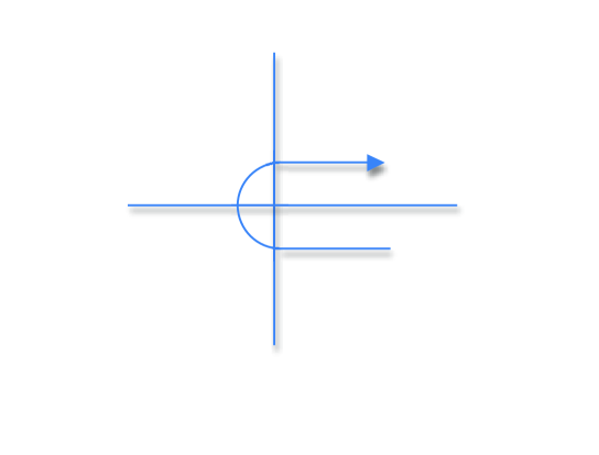
Figure 1: Contour of integration $C$.

$$g_{kl}(\omega,t)=\frac{1}{2\pi i}\int_{C}d\omega^{\prime}\,G_{kl}(\omega^{\prime})\,\frac{e^{-it\omega^{\prime}}}{\omega^{\prime}-\omega}\,,$$ (4.24)

where the contour $C$ is again the same as in (4.23). There exists the following relation between $A_{kl}(t)$ and $g_{kl}(\omega,t)$:

$$A_{kl}(t)=\left(i\frac{d}{dt}-\omega\right)\,g_{kl}(\omega,t)\,,$$ (4.25)

as it can be easily derived from (4.23) and (4.24).

In order to obtain the survival probability for the bound states of $H_{0}$, we just calculate the survival amplitude for these states. Let $|{\Phi}\rangle$ be the most general linear superposition of the eigenvectors of $H_{0}$, it has the following form:

$$|{\Phi}\rangle=\sum_{k=1}^{N}a_{k}\,|k\rangle\,.$$ (4.26)

Obviously, time evolution for (4.26) must have the following form

$$|{\Phi}(t)\rangle=\sum_{k=1}^{N}a_{k}\,|k\rangle_{t}\,.$$ (4.27)

We are now in the position of computing the survival amplitude $A(t)$ and hence the survival probability $|A(t)|^{2}$. For the survival amplitude, we have

$$A(t)=\langle\Phi|\Phi(t)\rangle=\sum_{k,k^{\prime}=1}^{N}a_{k}a^{*}_{k^{\prime}}\,\langle k|k^{\prime}\rangle_{t}=\sum_{k,k^{\prime}=1}^{N}a_{k}a^{*}_{k^{\prime}}\,A_{kk^{\prime}}(t)\,.$$ (4.28)

There is a form to write (4.28) as a sum of the contributions of the resonance poles plus the background. We need to change the contour $C$ into $C_{1}$ as depicted in Figure 2. Note that for this contour transformation we are using the idea that the analytic continuation from above to below is produced in the second sheet of a Riemann surface. With these ideas in mind, we obtain the following expression for $A_{kk^{\prime}}(t)$:

$$A_{kk^{\prime}}(t)=-\sum_{j}r^{j}_{kk^{\prime}}\,e^{-iz_{j}t}+\frac{1}{2\pi i}\int_{C_{1}}d\omega\,e^{-i\omega t}\,G_{kk^{\prime}}(\omega)\,.$$ (4.29)

Here the sum in $j$ runs out the poles of $G_{kk^{\prime}}(\omega)$ in the forth quadrant of the complex plane (see Figure .). The term $r^{j}_{kk^{\prime}}$ is the residue of $G_{kk^{\prime}}(\omega)$ at the pole $z_{j}$:

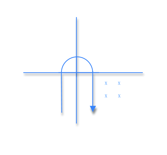
Figure 2: Contour of integration $C_{1}$. By x we represent the location of the resonance poles.

$$r^{j}_{kk^{\prime}}={\rm res\;}G_{kk^{\prime}}(\omega)\Big{|}_{\omega=z_{j}}\,.$$ (4.30)

Formula (4.29) can be written in a more explicit form, provided that we are assuming that the form factors $f_{k}(\omega)$ are analytically continuable into the lower half plane. After some calculations (given in [12] ), one obtains:

$$A_{kk^{\prime}}(t)=\sum_{j}N_{j}^{2}\,e^{-iz_{j}t}\sum_{k,l,k^{\prime},l^{\prime}=1}^{N}\lambda^{2}f_{l}(z_{j})\,f_{l^{\prime}}(z_{j})\,r^{j}_{kl}\,r^{j}_{k^{\prime}l^{\prime}}+\frac{1}{2\pi i}\int_{C_{1}}d\omega\,e^{-i\omega t}\,G_{kk^{\prime}}(\omega)\,,$$ (4.31)

where the $N_{j}$ are certain normalization constants [12].

The form of the terms $A_{kk^{\prime}}(t)$ and hence the form of the survival amplitude is particularly interesting. It has an oscillating term plus another term called the background and that is represented by the integral in (4.29) or (4.31). The background plays an essential role in the behavior of the decay phenomena at very short and very long values of time $t$. This behavior has been extensively studied [62, 45, 11, 48, 63, 77].

In the simplest Fridrichs model, $N=1$ and there is a simple pole resonance only located at $z_{0}$. Then, the form of $A(t)$ is simply

$$A(t)=-r\,e^{-itz_{0}}+\frac{1}{2\pi i}\int_{C_{1}}d\omega\,e^{-i\omega t}\,G(\omega)\,.$$ (4.32)

In this case, the survival probability $|A(t)|^{2}$ has a term that decays exponentially as $e^{-t\,{\rm Im\,}z_{0}}$ and that corresponds to the behavior of resonance phenomena for intermediate times, i. e., neither too short or two large [49]. However, if $N\geq 2$, the survival probability has an oscillating behavior for which the maximus decay as $t$ goes to infinite.

4.2 Two level model.

The simplest case of the $N$ level model is of course $N=2$. Also for simplicity, we have chosen the coupling constant $\lambda$ in $H=H_{0}+V$ equal to one, $\lambda=1$ This situation has already several interesting features and for this reason and also for its simplicity it is an example of obligatory study.

First of all, it is important to choose the form factors adequately. The following choice was proposed in the context of a study of decay for elementary particles [68]:

$$f_{k}(\omega)=\frac{\omega^{1/4}}{\omega+\rho_{k}^{2}}\;,\hskip 56.9055ptk=1,2\,,$$ (4.33)

where $\rho_{k}$ are positive numbers. These form factors permit to calculate the matrix elements $G^{-1}_{kk^{\prime}}(\omega)$ from (4.6) as

$$G^{-1}_{kk^{\prime}}(\omega)=(\omega_{k}-\omega)\delta_{kk^{\prime}}+\frac{\pi\lambda^{2}}{\rho_{k}+\rho_{k^{\prime}}}\;\frac{1}{(\sqrt{\omega}+i\rho_{k})(\sqrt{\omega}+i\rho_{k^{\prime}})}\,,$$ (4.34)

with $k,k^{\prime}=1,2$. The branch square root is defined so that a positive real number had a positive square root.

From (4.34) obtaining the $2\times 2$ matrix $G(\omega)$ is just a straightforward manipulation. In order to obtain the resonances as poles of $G(\omega)$ the technique will be to obtain these resonances as zeroes of the analytic continuation of the inverse of the determinant of the $2\times 2$ matrix $G(\omega)$. If we make the simple change of variables given by $\sqrt{\omega}=ix$, we need to solve the following equation in $x$:

$$(\det G(\omega))^{-1}=$$

$$\left[(\omega_{1}+x^{2})(x+\rho_{1})^{2}-\frac{\pi\lambda^{2}}{2\rho_{1}}\right]\times\left[(\omega_{2}+x^{2})(x+\rho_{2})^{2}-\frac{\pi\lambda^{2}}{2\rho_{2}}\right]-\left(\frac{\pi\lambda^{2}}{\rho_{1}+\rho_{2}}\right)^{2}$$

$$=0\,.$$ (4.35)

This is an algebraic equation of degree 8 with real coefficients. Therefore, all its roots are either real or appear in complex conjugate pairs. If certain conditions on $\omega_{i}$ and $\rho_{i}$ are fulfilled [12], $G(\omega)$ has no singularities except for a brunch cut coinciding with the positive semiaxis. Then, all the resonance poles are poles of the analytic continuation, or in the language of Riemann surfaces, they are located in the second Riemann sheet. Real singularities correspond to virtual poles and lie in the negative semiaxis (second sheet).

In the case of weak coupling, i. e., when the coupling constant $\lambda$ is very small, two pairs of complex conjugate poles can be evaluated perturbatively. The result is given by:

$$z_{j} = \omega_{j}+\frac{\pi\lambda^{2}}{2\rho_{j}}\;\frac{(\sqrt{\omega_{j}}-i\rho_{j})^{2}}{(\omega_{j}+\rho_{j}^{2})^{2}}+\frac{\pi^{2}\lambda^{4}}{(\sqrt{\omega_{j}}+i\rho_{j})^{2}}$$ (4.36)

$$\times \left(\frac{1}{(\omega_{j}-\omega_{k})(\rho_{1}+\rho_{2})^{2}(\sqrt{\omega_{j}}+i\rho_{k})^{2}}-\frac{1}{4\rho_{j}^{2}\,\sqrt{\omega_{j}}\,(\sqrt{\omega_{j}}+i\rho_{j})^{2}}\right)$$

$$+ o(\lambda^{6})\,,\quad j=1,2\,,\quad k\neq j\,.$$

In this case, we can obtain approximate expressions for the real and imaginary parts of $z_{j}$ and the result is given by

$$\widetilde{\omega}:={\rm Real}\,z_{j}=\omega_{j}+\frac{\pi\lambda^{2}}{2\rho_{j}}\;\frac{\omega_{j}-\rho_{j}^{2}}{(\omega_{j}+\rho_{j}^{2})^{2}}+o(\lambda^{4})\,,\quad j=1,2\,,$$

$$\gamma_{j}:=-{\rm Im}\,z_{j}=\frac{\pi\lambda^{2}\,\sqrt{\omega_{j}}}{(\omega_{j}+\rho_{j}^{2})^{2}}+o(\lambda^{4})\,,\quad j=1,2\,.$$ (4.37)

Note that (4.35) is of eight degree, so that it must have eight solutions. We have already calculated four of them. The other four are real and correspond to virtual states [12], also called anti-bound states.

Then, (4.37) permits us to write an approximate expression for the survival amplitud $A(t)$. If we neglect the background term, (4.37) yields [12]

$$A(t) \approx \sum_{k,k^{\prime}=1,2}a_{k}a_{k^{\prime}}^{*}\sum_{j=1,2}e^{-\gamma_{j}t}\,e^{-i\widehat{\omega}t}\,r_{kk^{\prime}}^{j}$$

$$= \sum_{j=1}^{2}|a_{j}|^{2}\,e^{-iz_{j}t}-\lambda^{2}\sum_{j=1}^{2}\left(\frac{i\pi|a_{j}|^{2}\,e^{-iz_{j}t}}{2\rho_{j}(\rho_{j}-i\sqrt{\omega_{j}})^{3}\,\sqrt{\omega_{j}}}\right.$$

$$+ \left.\frac{2\pi\,{\rm Real}\,(a_{1}a_{2}^{*})\,e^{-iz_{j}t}}{(\rho_{1}+\rho_{2})(\rho_{j}-i\sqrt{\omega_{j}})(\rho_{l}-i\sqrt{\omega_{j}})(\omega_{j}-\omega_{l})}\right)+o(\lambda^{4})\,\quad l\neq j\,.$$

It is important to remark that both in (4.36) and (LABEL:n38) the term $1/(\omega_{k}-\omega_{l})$ appears. Then, these expressions cannot be used in the case of the existence of degeneracy levels for $H_{0}$.

Note that, although for some initial conditions like $a_{1}=1$, $a_{2}=0$, the survival amplitude (LABEL:n38) does not show oscillations, these oscillations must be present in the terms of the order $\lambda^{4}$. For the lowest order $\lambda^{2}$, the survival probability can be written in the following form

$$|A(t)|^{2}=|\,|a_{1}|^{2}\,e^{-\gamma_{1}t}+|a_{2}|^{2}\,e^{-\gamma_{2}t}\,e^{-2i\nu t}|^{2}\,,$$ (4.39)

with

$$\nu:=\frac{\widetilde{\omega}_{1}-\widetilde{\omega}_{2}}{2}\;.$$ (4.40)

From (4.39), we can see the dependence of the survival probability with respect to the initial conditions. For $a_{1}=0$ or $a_{2}=0$, the survival probability behaves exponentially without oscillations, at this order of approximation. If $a_{1}\approx a_{2}$ the survival probability shows considerable oscillations.

4.3 The $N$-level model.

An analysis can be carried out for the $N$ level model in the weak coupling regime. We can use arbitrary form factors $f_{k}(\omega)$ in (4.7). Then, we can get

$$(\det G(\omega))^{-1}=\prod_{k=1}^{N}(\omega_{k}-\omega)-\lambda^{2}\sum_{k=1}^{N}I_{kk}(\omega)\prod_{m\neq k}^{N}(\omega_{m}-\omega)+o(\lambda^{4})\,,$$ (4.41)

where

$$I_{kl}(\omega)=\int_{0}^{\infty}d\omega^{\prime}\,\frac{f_{k}(\omega^{\prime})\,f_{l}(\omega^{\prime})}{\omega^{\prime}-\omega-i0}\;.$$ (4.42)

The zeroes of (4.41) give the position of the resonances:

$$z_{k}=\omega_{k}-\lambda^{2}I_{kk}(\omega_{k})+o(\lambda^{4})=\widetilde{\omega}_{k}-i\gamma_{k}\,,\quad j=1,2,\dots,N\,,$$ (4.43)

where, again, $\widetilde{\omega}_{k}={\rm Real}\,z_{k}$ and $\gamma_{k}={\rm Im}\,z_{k}$.

Then, in the first nontrivial order, which is $\lambda^{2}$, we have for the real and imaginary part of the resonance pole located at $z_{k}$ the following expression:

$$\widetilde{\omega}_{k}=\omega_{k}\;,\hskip 56.9055pt\gamma_{k}=\pi\lambda^{2}\,f_{k}^{2}(\omega_{k})\;.$$ (4.44)

It is not a surprise that, at first order, real parts of $z_{k}$ do not depend on $\lambda$, while imaginary parts depend on $\lambda^{2}$. This is exactly what happens in the two level model studied in the previous subsection, see (4.36). At this order of approximation, we can also calculate the partial resolvent $G$ [12]

$$G_{kk^{\prime}}(\omega)=(\omega_{k}-\omega-\lambda^{2}I_{kk^{\prime}}(\omega)\,)^{-1}\,\delta_{kk^{\prime}}+o(\lambda^{2})\,,$$ (4.45)

the residues

$$r_{kk^{\prime}}^{j}=-\delta_{kk^{\prime}}\delta_{kj}+o(\lambda^{2})$$ (4.46)

and the survival amplitude

$$A(t)=\sum_{k=1}^{N}|a_{k}|^{2}\,e^{-i\omega_{k}t}\,e^{-\pi\lambda^{2}f_{k}^{2}(\omega_{k})t}\;.$$ (4.47)

The conclusion that one arrives is that, although the survival probability decays, the decaying mode can be strongly oscillatory, depending on the values of the parameters $a_{k}$, $k=1,2,\dots,N$ (initial conditions). One study of particular forms of this decay can be seen in [12].

5 Some types of Friedrichs-like models and their applications to Quantum Field Theory.

More sophisticated versions of the Friedrichs model have been used to introduced models for unstable relativistic quantum fields exactly solvable on a sector or under a well determined simplification or approximation. We want to discuss a few models that have been introduced elsewhere [9, 8, 61, 5, 6] that are very useful to give us an idea on the construction and behavior of relativistic resonances, not making use of the $S$ matrix formalism (for a study on relativistic resonances in the context of the $S$ matrix see [28, 29, 31]).

Along this section, we are going to present four different situations, which are somehow related with unstable quantum field theory. In the first one, we consider two local fields with a cubic interaction. We show that, although the model is in principle not exactly solvable, it can be solved in a sector in which a particle of one of the spices considered decays into two of the other spice. In the second one, the interaction is between a local quantum field and a bilocal quantum field with a continuous and bounded mass spectrum. We choose a quadratic interaction between these two fields, which makes the exact solution tractable through a rather complicated generalization of the Friedrichs model. Due to the complexity of this example, we shall limit ourselves to give here a summary of it. Readers interested in a deeper understanding of this example can go to the original paper [9]. Finally, we propose an example of “second quantized Friedrichs model”, the Friedrichs model with virtual transitions, which is probably the simplest case of these second quantized models.

5.1 First model.

Assume that we have two real scalar relativistic quantum fields $\varphi(x)$ and $\psi(x)$, where $x$ is the fourth component space time, with respective masses given by $m$ and $M$, coupled with the simplest cubic interaction. The Hamiltonian of the system is given by

$$H=H_{m}+H_{M}+V\,,$$ (5.1)

where

$$H_{m} = \int dx\,(\dot{\varphi}^{2}+(\nabla\varphi)^{2}+m^{2}\varphi^{2})$$ (5.2)

$$H_{M} = \int dx\,(\dot{\psi}^{2}+(\nabla\psi)^{2}+M^{2}\psi^{2})$$ (5.3)

$$V = \lambda\int dx\psi(x)\varphi^{2}(x)\,.$$ (5.4)

The dot means first derivative with respect to time. By boldface letters we denote three-dimensional vectors. Four-dimensional vectors in Minkowski space are denoted by roman style letters. The products of two four vectors as well as the scalar products of two three vectors are denoted by a dot. We use the standard metric $(+,-,-,-)$ of Minkowski space. For example: $k\cdot x=k_{0}x_{0}-{\bf k}\cdot{\bf x}$.

In terms of the creation and annihilation operators, the above formulae can be written in the interaction picture as:

$$H_{m} = \int d\widetilde{\bf q}\,\rho({\bf q})b^{\dagger}({\bf q})b({\bf q})$$ (5.5)

$$H_{M} = \int d\widetilde{\bf k}\,\omega({\bf k})a^{\dagger}({\bf k})a({\bf k})$$ (5.6)

$$V_{I}(t) = \lambda\int d\widetilde{\bf k}\,d\widetilde{\bf q}_{1}\,d\widetilde{\bf q}_{2}\,\int d^{3}{\bf x}\,[a^{\dagger}({\bf k})\,\exp(ik\cdot x)+a({\bf k})\,\exp(-ik\cdot x)]$$ (5.7)

$$\times [b^{\dagger}({\bf q}_{1})\,\exp(iq_{1}\cdot x)+b({\bf q}_{1})\,\exp(-iq_{1}\cdot x)]$$

$$\times [b^{\dagger}({\bf q}_{2})\,\exp(iq_{2}\cdot x)+b({\bf q}_{2})\,\exp(-iq_{2}\cdot x)]\,.$$

The quantum field operators in (5.2-5.4) are given by

$$\psi({\bf x},t) = \int d\widetilde{\bf k}\,[a^{\dagger}({\bf k})\,\exp(ik\cdot x)+a({\bf k})\,\exp(-ik\cdot x)]$$

$$\varphi({\bf x},t) = \int d\widetilde{\bf q}\,[b^{\dagger}({\bf q})\,\exp(iq\cdot x)+b({\bf q})\,\exp(-iq\cdot x)]$$ (5.8)

with the Lorentz invariant measure

$$d\widetilde{\bf k} = \frac{d^{3}{\bf k}}{(2\pi)^{3}2\omega({\bf k})}\,,\hskip 28.45274pt\omega({\bf k})=({\bf k}^{2}+M^{2})^{1/2}$$

$$d\widetilde{\bf q} = \frac{d^{3}{\bf q}}{(2\pi)^{3}2\rho({\bf q})}\,,\hskip 28.45274pt\rho({\bf q})=({\bf q}^{2}+m^{2})^{1/2}\;.$$ (5.9)

The creation and annihilation operators in (5.5-5.7) satisfy the usual commutation relations:

$$[a({\bf k}),a^{\dagger}({\bf k}^{\prime})] = (2\pi)^{3}2\omega({\bf k})\delta({\bf k}-{\bf k}^{\prime})$$

$$[b({\bf q}),b^{\dagger}({\bf q})] = (2\pi)^{3}2\rho({\bf q})\delta({\bf q}-{\bf q}^{\prime})\,.$$ (5.10)

The first goal is to obtain an appropriate asymptotic dynamics for this situation. Note that scattering theory applies if asymptotic completeness holds true between the free and the interacting fields [22]. If this assumption is not valid, one tries to find another solvable evolution which satisfies the asymptotic condition and reestablish scattering theory as a comparison between the interaction field and the redefined asymptotic field. A typical example is the Faddeev-Kulish [46] removal of infrared divergencies.

After integration over the three dimensional space, i.e., with respect to $d^{3}{\bf x}$, on the right hand side of (5.7), we obtain eight terms of products of creation and annihilation operators with $t$-dependent exponents accomplished with three dimensional $\delta$ functions of momentum conservation. According to the Riemann-Lebuesgue lemma [87], the asymptotic behavior of $V_{I}(t)$ is defined by the behavior of these $t$-dependent exponents in the integration domain. For example, one of the terms on the right hand side of (5.7) is

$$\int d\widetilde{\bf k}\,d\widetilde{\bf q}_{1}\,d\widetilde{\bf q}_{2}\,a^{\dagger}({\bf k})\,b({\bf q}_{1})\,b({\bf q}_{2})\,\exp(i[\omega({\bf k})-\rho({\bf q}_{1})-\rho({\bf q}_{2})]t)(2\pi)^{3}\,\delta({\bf k}+{\bf q}_{1}+{\bf q}_{2})\,.$$ (5.11)

The asymptotic behavior of the integral (5.11) as $t\longmapsto\pm\infty$ is determined by the term $[\omega({\bf k})-\rho({\bf q}_{1})-\rho({\bf q}_{2})]$. Notice that

$$\omega({\bf k})+\rho({\bf q}_{1})+\rho({\bf q}_{2})\bigg{|}_{{\bf k}+{\bf q}_{1}+{\bf q}_{2}={\bf 0}}\geq M+2m>0\,.$$ (5.12)

Therefore, the integral (5.11) goes rapidly to zero due to the fast oscillations (indeed to the Riemann-Lebesgue lemma). Let us consider another term

$$\int d\widetilde{\bf k}d\widetilde{\bf q}_{1}d\widetilde{\bf q}_{2}\;a^{\dagger}({\bf k})b({\bf q}_{1})b({\bf q}_{2})e^{i[\omega({\bf k})-\rho({\bf q}_{1})-\rho({\bf q}_{2})]t}\,(2\pi)^{3}\,\delta({\bf k}-{\bf q}_{1}-{\bf q}_{2})\,.$$ (5.13)

As for the case of the previous integral (5.11), the asymptotic behavior of (5.13) is defined by the quantity

$$\Delta({\bf k},{\bf q}_{1})=\omega({\bf k})-\rho({\bf q}_{1})-\rho({\bf q}_{2})\bigg{|}_{{\bf k}-{\bf q}_{1}-{\bf q}_{2}=0}\,.$$ (5.14)

The values of $\Delta({\bf k},{\bf q}_{1})$ depend on the masses of the fields $\varphi$ and $\psi$. If $M<2m$, then $\Delta({\bf k},{\bf q}_{1})$ is strictly negative:

$$\Delta({\bf k},{\bf q}_{1})\leq 2(m^{2}+\frac{{\bf k}^{2}}{4})^{1/2}-(M^{2}+{\bf k}^{2})^{1/2}<0\,.$$ (5.15)

To show (5.15), we obtain the maximum of $\Delta({\bf k},{\bf q}_{1})$ on ${\bf q}_{1}$ for each $\bf k$. This maximum is at ${\bf q}_{1}={\bf k}/2$ (it is certainly a maximum) and the value of $\Delta({\bf k},{\bf q}_{1})$ at the maximum is

$$2(m^{2}+\frac{{\bf k}^{2}}{4})^{1/2}-(M^{2}+{\bf k}^{2})^{1/2}\,.$$ (5.16)

Note that if $M<2m$, (5.16) is indeed smaller than zero. Thus, $\Delta({\bf k},{\bf q}_{1})$ has constant sign and therefore the Riemann-Lebesgue lemma applies. As a consequence, the integral (5.13) decreases fast as $t\longmapsto\pm\infty$.

In contrast, let us assume that $M>2m$. Then the maximum (5.13) is bigger than zero. However, for fixed $\bf k$ the term

$$\Delta({\bf k},{\bf q}_{1})=(M^{2}+{\bf k}^{2})^{1/2}-(m^{2}+{\bf q}^{2}_{1})-(m^{2}+({\bf q}_{1}-{\bf k})^{2})^{1/2}$$ (5.17)

is obviously smaller than zero for high values of $|{\bf q}_{1}|$. Let us consider the manifold for which

$$\Delta({\bf k},{\bf q}_{1})=0\,.$$ (5.18)

The integral (5.13) over this region does not vanish asymptotically and the same behavior can be observed on its complex conjugate. In other words, by relinquishing the stability condition $M<2m$, we obtain an unstable field theory where the asymptotic condition for scattering theory fails. Therefore, following a standard procedure in field theory, we redefine the asymptotic evolution in the interaction picture as follows:

$$h_{as}=H_{0}+V_{as}(t)\;,$$ (5.19)

where $V_{as}$ includes the slowly decreasing part of $V_{I}$. There is an ambiguity in the definition of $V_{as}$ and we shall take it as the sum of (5.13) and its complex conjugate, so that $V_{as}$ is Hermitian. This is the simplest choice for $V_{as}$:

$$V_{as}(t) = \lambda\int d\widetilde{\bf k}\,d\widetilde{\bf q}_{1}\,d\widetilde{\bf q}_{2}\;[a^{\dagger}({\bf k})b({\bf q}_{1})b({\bf q}_{2})e^{i\Delta({\bf k},{\bf q}_{1})t}+$$ (5.20)

$$+ a({\bf k})b^{\dagger}({\bf q}_{1})b^{\dagger}({\bf q}_{2})e^{-i\Delta({\bf k},{\bf q}_{1})t}](2\pi)^{3}\,\delta({\bf k}-{\bf q}_{1}-{\bf q}_{2})$$

$$= \lambda\int d^{3}{\bf x}[\psi^{(+)}(x)\varphi^{(-)2}(x)+\psi^{(-)}(x)\varphi^{(+)2}(x)]\,,$$

where $\Delta$ was defined in (5.14) and $\varphi^{(+)},\varphi^{(-)}$ denote the positive and negative frequency parts of $\varphi$. Same for $\psi$.

• The above comments have an obvious physical interpretation: The decay process given by

  $$\psi\longmapsto\varphi+\varphi$$

  is only possible if the mass $M$ of the $\psi$-particle is bigger than the mass $2m$ corresponding to two $\varphi$-particles.

• Renormalization. As we shall see below the $h_{as}$ produces a ultraviolet divergence in the equation for its eigenstates. In order to remove this divergence we add to $h_{as}$ the appropriate counterterm

  $$H_{c.t.}=\frac{1}{2}\int d^{3}x\,\delta M^{2}\varphi^{(+)}(x)\varphi^{(-)}(x)=\int d{\bf k}\;\frac{\delta M^{2}}{\omega({\bf k})}\;a^{\dagger}({\bf k})\,a({\bf k})\,,$$ (5.21)

  where the mass renormalization $\delta M^{2}$ is of order $\lambda^{2}$. The appearance of ultraviolet counterterms is due to our choice of the asymptotic interaction. We can of course introduce some smooth cut off in $V_{as}$, but it will involve additional parameters to the asymptotic states and it will generally break the relativistic invariance of the system.

In order to obtain the desired formula for the asymptotic Hamiltonian, we add $h_{as}$ and $H_{c.t.}$:

$$H_{as}(t)=h_{as}(t)+H_{c.t.}\,.$$ (5.22)

In the Schrödinger picture, the time dependent exponents $e^{\pm i\Delta(k,q_{1})t}$ in equation (5.20) disappear. Now, we shall consider the eigenstates of $H_{as}=H_{as}(0)$, which is a Hermitian operator in the Fock space corresponding to the creation and annihilation operators satisfying (5.10).

From now on, we shall work in the Schrödinger picture, in order to make calculations easier. In the Schrödinger picture the total Hamiltonian $H$ will be the following:

$$H_{as}=H_{M}+H_{m}+H_{c.t.}+\lambda\int d\widetilde{\bf k}\,d\widetilde{\bf q}_{1}\,d\widetilde{\bf q}_{2}\;[a^{\dagger}({\bf k})b({\bf q}_{1})b({\bf q}_{2})$$

$$+a({\bf k})b^{\dagger}({\bf q}_{1})b^{\dagger}({\bf q}_{2})]\,(2\pi)^{3}\,\delta({\bf k}-{\bf q}_{1}-{\bf q}_{2})\,.$$ (5.23)

We shall show how the above problem of unstable quantum field can be solved exactly on a sector. Of course, as the interaction is not quadratic, no exact solution is know for all sectors. This sector corresponds to the decay of one $\psi$-particle into two $\varphi$-particles. The Hilbert space of this system is given by

$${\cal H}:={\cal H}_{\varphi}\otimes{\cal H}_{\varphi}\oplus{\cal H}_{\psi}\,.$$ (5.24)

The eigenspaces of the operator

$$N=N_{\psi}+2N_{\varphi}$$ (5.25)

are invariant subspaces of $H_{as}$. The operators $N_{\psi}$ and $N_{\varphi}$ are the number operators of $\psi$ and $\varphi$-particles. The asymptotic interaction does not affect the vacuum state and the one $\psi$-particle state, which are the only nondegenerate eigenspaces of $N$. The first degenerate case is the eigenspace of $N$ with eigenvalue $2$, which is precisely $\cal H$ as given in (5.23). In the subspace (5.23) the term $V_{as}$ in $H_{as}$ produces transitions of two $\varphi$-particles state to one $\psi$-particle and vice versa. We should mention that not every two $\varphi$-particle state will mix with one $\psi$-particle state, but only with those in which the two $\varphi$-particles are in the $S$-wave state.

The most general linear combination of two $\varphi$-particles in the $S$-wave state with one $\psi$-particle, can be written as:

$$\Phi(E,{\bf k})=f(E,{\bf k})|{\bf k}\rangle+\int dE^{\prime}\,f(E,E^{\prime},{\bf k})|E^{\prime},{\bf k}\rangle\,,$$ (5.26)

where $|E^{\prime},{\bf k}\rangle$ is the two $\varphi-$particle $S-$wave and $|{\bf k}\rangle$ is the one $\psi$ particle state. The objective is to solve the eigenvalue equation

$$(H_{as}-E)\Phi(E,{\bf k})=0\,,$$ (5.27)

where $H_{as}$ was given in (5.23). The method to solve this equation consists in replacing (5.26) into (5.27). Thus, we can obtain the coefficients $f(E,{\bf k})$ and $f(E,E^{\prime},{\bf k})$.

We are interested in obtaining these coefficients in the unstable case characterized by the condition $M>2m$, where $M$ and $m$ are the respective masses of the $\psi$ and $\varphi$ particles. The method is tricky as it requieres the use of “counterterms” and a particular choice of a normalization, but it is explained in detail in [8]. The final result is given by

$$f(E,{\bf k})=-A\,\frac{1}{\eta(E,{\bf k})}\,\frac{\lambda\sqrt{2}}{2\omega({\bf k})}\,\tau(E^{2}-{\bf k}^{2})$$ (5.28)

and

$$f(E,E^{\prime},{\bf k})=A\left\{\delta(E^{\prime}-E)+\frac{2\lambda^{2}(2\pi)^{3}}{2\omega({\bf k})}\,\frac{\tau(E^{2}-{\bf k}^{2})}{\eta(E,{\bf k})}\,\frac{1}{E^{\prime}-E}\right\}\;,$$ (5.29)

where

$$\langle{\bf k}|\frac{1}{H_{as}-E}|{\bf k}\rangle=\frac{1}{\eta(E,{\bf k})}$$ (5.30)

is the partial resolvent of the Hamiltonian $H_{as}$. This partial resolvent has an explicit expression [6]. The function $\tau$ is defined on the halfline $E>(4m^{2}+{\bf k}^{2})^{1/2}$ by

$$\tau(E^{2}-{\bf k}^{2}) = \int d\widetilde{\bf q}_{1}d\widetilde{\bf q}_{2}\delta({\bf k}-{\bf q}_{1}-{\bf q}_{2})\delta(E-\rho({\bf q}_{1})-\rho({\bf q}_{2}))$$

$$= \frac{1}{4(2\pi)^{5}}\left(1-\frac{4m^{2}}{E^{2}-{\bf k}^{2}}\right)^{1/2}\theta(E-(4m^{2}+{\bf k}^{2})^{1/2})\;,$$

where $\theta(x)$ is the usual Heaviside step function, $d\widetilde{\bf q}_{i}$ and $\omega({\bf k})$ were defined in (5.9) and $A$ is an arbitrary constant.

In (5.29) there is an ambiguity which arises due to the singular denominator $(E^{\prime}-E)$. This ambiguity also exists in (5.28) although it is there hidden in the partial resolvent (5.30). Consequently, we shall define two solutions of eigenvalue problem (5.27) that correspond to the incoming and the outgoing solution. The incoming and outgoing solutions are defined as boundary functions of analytic functions from above $(E+i0)$ and from below $(E-i0)$ the real axis respectively:

$$\Phi^{in\atop out}(E,{\bf k}) = A\left\{|E,{\bf k}\rangle+\frac{\lambda\sqrt{2}\cdot\tau(E^{2}-{\bf k})}{2\omega({\bf k})\eta(E\pm i0,{\bf k})}\times\right.$$

$$= \left.\times[\lambda\sqrt{2}\cdot(2\pi)^{3}\int_{E_{0}}^{\infty}dE^{\prime}\frac{1}{E^{\prime}-E\mp i0}|E^{\prime},{\bf k}\rangle-|{\bf k}\rangle]\right\}.$$

This formula explicitly demonstrates that the energy spectrum of the asymptotic states in the eigenspace of $N$, as defined in (5.25), corresponding to the eigenvalue 2, is absolutely continuous over the interval $[E_{0},\infty)$ where $E_{0}=(4m^{2}+{\bf k}^{2})^{1/2}$. The isolated eigenvalue associated to the one $\psi$-particle state $|{\bf k}\rangle$ has been dissolved to the continuum due to the interaction. This reproduces somehow the situation that appears in the standard Friedrichs model discussed in Section 2.

5.1.1 The Gamow vectors.

In [6], it has been shown that the inverse partial resolvent $\eta(E,{\bf k})$ admits a continuation on the variable $E$, $\eta_{+}(E,{\bf k})$, from above to below through the branch cut $[E_{0},\infty)$ and has a complex zero $z_{R}$ on the lower halfplane. In order to find resonances, we have to solve the equation $\eta(E,{\bf k})=0$. The explicit form of $\eta(E,{\bf k})$ is

$$\eta(E,{\bf k})=\omega({\bf k})-E-\lambda^{2}(2\pi)^{3}(E-a)\int_{E_{0}}^{\infty}dE^{\prime}\,\frac{\tau({E^{\prime}}^{2}-{\bf k}^{2})}{(E^{\prime}-E)(E^{\prime}-a)}\,,$$ (5.33)

where $\tau({E^{\prime}}^{2}-{\bf k}^{2})$ was given in (LABEL:ac).

Note that the interaction $V_{as}$ in (5.20) depends on a multiplicative coupling constant $\lambda$. When $\lambda=0$, the interaction is switched off, exactly as it happens in the ordinary Friedrichs model. It has been shown in [6] that in absence of interaction ($\lambda=0$), $E=\omega({\bf k})$ and that for small values of $\lambda$ one has that the solution of the equation $\eta(E,{\bf k})=0$ corresponding to the lower half plane should have the following form

$$z_{R}=\omega({\bf k})+\lambda^{2}z_{1}+O(\lambda^{4})\,,$$ (5.34)

where

$$z_{1}=-\frac{i}{8\pi}\left(1-\frac{4m^{2}}{M^{2}}\right)^{1/2}\,.$$ (5.35)

Note that (5.9) shows that $M^{2}=\omega^{2}({\bf k})-{\bf k}^{2}$, where $M$ is the mass of the $\psi-$particle. Then, (5.34) and (5.35) gives

$$z_{R}=\omega({\bf k})-i\frac{M\Gamma}{2\omega({\bf k})}\simeq({\bf k}^{2}+M^{2}-iM\Gamma)^{1/2}\,,$$ (5.36)

where we have denoted

$$M\Gamma=\frac{\lambda^{2}}{8\pi}\left(1-\frac{4m^{2}}{M^{2}}\right)^{1/2}\,.$$ (5.37)

This zero has a complex conjugate on the analytic continuation from above to below. Equation (5.36) demonstrates that the zero of $\eta(E,{\bf k})$ corresponds to a particle with complex square mass

$$M^{2}_{c}=M^{2}-iM\Gamma\,,$$ (5.38)

which is the remnant of a $\psi$-particle. The eigenstate (LABEL:ad) as a function of $E$ has a pole at the point $E=z_{R}$ and its residue in this pole is the eigenstate with complex energy. Up to an irrelevant normalization constant this state is:

$$\Phi^{G}(z_{R},{\bf k})=\lambda\sqrt{2}\cdot(2\pi)^{3}\int_{E_{0}}^{\infty}dE^{\prime}\frac{1}{E^{\prime}-z_{R}}|E^{\prime},{\bf k}\rangle-|{\bf k}\rangle\,.$$ (5.39)

This Gamow vector has a clear meaning as an antilinear functional on a suitably chosen space of test functions $\bf\Phi$. The test function space should be dense on the Hilbert space (5.24) of the states of two $\varphi$-particles and one $\psi$-particle, which is contained in the Fock space of the states of $\varphi$ particles and $\psi$-particles. Following the spirit of the construction for simple non relativistic resonances, a simple choice for the test function space, dense in the Hilbert space (5.24), is given by

$${\bf\Phi}:=[({\cal H}^{2}_{-}\cap S)\otimes S({\mathbb{R}}^{3})]\oplus S({\mathbb{R}}^{3})\,.$$ (5.40)

We recall that

• ${\cal H}^{2}_{-}$ is the space of Hardy functions on the lower half plane.

• $S$ is the space of all real valued complex functions that are differentiable at all orders such that they as well as their derivatives vanish at the infinity faster than the inverse of any polynomial (the one dimensional Schwartz space).

• $S({\mathbb{R}}^{3})$ represents the space of all complex functions on the three dimensional real space ${\mathbb{R}}^{3}$ having the same properties as the Schwartz space $S$.

Then, the rigged Hilbert space is a triplet of the form ${\bf\Phi}\subset{\cal H}\subset{\bf\Phi}^{\times}$, where ${\bf\Phi}^{\times}$ is the dual space of $\bf\Phi$. Then, Gamow vectors belong to this dual ${\bf\Phi}^{\times}$.

A typical function in $\bf\Phi$ has the form $F(E,{\bf k})+g({\bf k^{\prime}})$ where $F(E,{\bf k})\in({\cal H}^{2}_{-}\cap S)\otimes S({\mathbb{R}}^{3})$ and $g({\bf k^{\prime}})\in S({\mathbb{R}}^{3})$. The variables $E$ and $\bf k$ in $F(E,{\bf k})$ represents respectively the total energy and the sum of the momenta for the two $\varphi$-particles. The variable $\bf k^{\prime}$ is the momentum of the $\psi$-particle.

The action of the functional (5.39) on the function $K(E,{\bf k^{\prime\prime}},{\bf k^{\prime}}):=F(E,{\bf k^{\prime\prime}})$ $+g({\bf k^{\prime}})$ is given by

$$\langle K(E,{\bf k^{\prime\prime}},{\bf k^{\prime}})|\Phi^{G}(z_{R},{\bf k})\rangle = \lambda\sqrt{2}\cdot(2\pi)^{3}\,\int_{E_{0}}^{\infty}dE^{\prime}\frac{1}{E^{\prime}-z_{R}}\langle F(E,{\bf k^{\prime\prime}})|E^{\prime},{\bf k}\rangle$$

$$-\langle g({\bf k^{\prime}})|{\bf k}\rangle = \lambda\sqrt{2}\cdot(2\pi)^{3}\,\int_{E_{0}}^{\infty}dE^{\prime}\,\frac{F(E,{\bf k})}{E^{\prime}-z_{R}}+g({\bf k})\;.$$ (5.41)

For the fixed variable $\bf k$, the function $F(E,{\bf k})$ is a Hardy function and, therefore, the integral term of (5.41) converges. In the usual Fock space notation, a typical element of ${\bf\Phi}^{\times}$ can be written as

$$F(E,{\bf k^{\prime\prime}})\,|E,{\bf k}^{\prime\prime}\rangle+g({\bf k^{\prime}})|{\bf k}^{\prime}\rangle\,.$$ (5.42)

The functional $\Phi^{G}(z_{R},{\bf k})$ has the following property:

$$H_{as}\,\Phi^{G}(z_{R},{\bf k})=z_{R}\,\Phi^{G}(z_{R},{\bf k})\,.$$ (5.43)

It may be interesting to discuss the proof of this latter statement. We have seen that $\Phi(E,{\bf k})$ has a meromorphic extension from above to below on the variable $E$ with a pole at the point $z_{R}$. Lets us call this extension $\Phi_{C}(z,{\bf k})$. The residue of $\Phi_{C}(z,{\bf k})$ at $z_{R}$ gives the Gamow vector $\Phi^{G}(z_{R},{\bf k})$. On a neighborhood of $z_{R}$ one has the following expansion in terms of the complex energy $z$:

$$\Phi_{C}(z,{\bf k})=\frac{1}{z-z_{R}}\Phi^{G}(z_{R},{\bf k})+{\rm regular}\;\;{\rm terms}\,.$$ (5.44)

The meromorphic extension of $\Phi(E,{\bf k})$ allows us to extend (5.27), so that, we have:

$$H_{as}\Phi_{C}(z,{\bf k})=z_{R}\,\Phi_{C}(z,{\bf k})\,,$$ (5.45)

for values of the complex energy $z$ in the lower half plane. If we bring (5.45) into (5.44), we get:

$$\frac{H_{as}\Phi^{G}(z_{R},{\bf k})}{z-z_{R}}+{\rm regular}\;\;{\rm terms}=(z-z_{R}+z_{R})\,\frac{\Phi^{G}(z_{R},{\bf k})}{z-z_{R}}+{\rm regular}\;\;{\rm terms}\,.$$ (5.46)

If we identify the pole terms in the left and right hand sides of (5.46), we finally arrive to (5.42). This concludes the presentation of the model.

5.2 Resonances in the interaction between a local and a bilocal boson field.

In this example, developed in [9], we shall consider an exactly solvable model for relativistic unstable quantum fields. This model considers a quadratic interaction between a local scalar field $\varphi$ with a mass $M$ and a bilocal scalar field $\psi$ with a continuous mass spectrum (we shall explain this terminology soon). The interaction makes the local scalar field unstable. The interaction is exactly solvable and it can be worked out as a generalization of the Friedrichs model.

It is very convenient to write the local scalar field $\varphi(x)$ with mass $M$ in terms of the creation and annihilation operators as follows:

$$\varphi({\bf x},t)=\int d\widetilde{\bf k}\,[a^{\dagger}({\bf k})\,e^{ik\cdot x}+a({\bf k})\,e^{-ik\cdot x}\,]\,.$$ (5.47)

Note that $k=(k_{0},{\bf k})$ and $x=(x_{0},{\bf x})$. By boldface letters we always denote three dimensional vectors. Four dimensional vectors in in Minkowski space are denoted by Roman style letters. The products of two vectors in Minkowski space are characterized by a dot. In Minkowski space we use the metric $+---$. For example, $k\cdot x=k_{0}x_{0}-{\bf kx}$. The Lorentz invariant measure $d\widetilde{\bf k}$ was defined in (5.9).

The creation and annihilation operators in (5.47) satisfy the following commutation relations:

$$[a({\bf k}),a^{\dagger}({\bf k})]=(2\pi)^{3}\,2\,\omega(({\bf k})\,\delta({\bf k}-{\bf k^{\prime}})\,.$$ (5.48)

The Hamiltonian for the field $\varphi(x)$ is given by

$$H_{m}=\int d\widetilde{\bf k}\,\omega(({\bf k})\,a^{\dagger}({\bf k})\,a({\bf k})\,.$$ (5.49)

Therefore, the field $\varphi(x)$ is a free Klein-Gordon field.

Next, we consider a bilocal scalar field $\psi(x_{\mu},q)$ with continuous mass spectrum and we shall describe this field as follows. Apart from the dependence of $\psi$ on the four vector $x$ with components $x_{\mu}$, $\mu=0,1,2,3$, it depends on an additional real variable $q$ representing an internal degree of freedom.

For simplicity in our calculations and because it does not interfere in our discussion, we shall assume that $\psi(x_{\mu},q)$ is an even function of $q$. This means that

$$\psi(x_{\mu},q)=\psi(x_{\mu},-q)\,.$$ (5.50)

The mass operator affects to this internal variable and in its simplest form has the form

$${\bf M}^{2}=4m-\frac{\partial^{2}}{\partial q^{2}}\,.$$ (5.51)

Then, the field $\psi(x_{\mu},q)$ satisfies the following generalized Klein-Gordon equation:

$$(\Box-{\bf M}^{2})\,\psi(x_{\mu},q)=0\,,$$ (5.52)

where $\Box$ is the usual D’Alembert operator.

Bilocal fields were introduced by Yukawa [102] and Markov [71] in connection with extended particles. The motivation of its use here is described in [6] in which the solution $\psi(x_{\mu},q)$ of (5.52) can be seen as the state of two particles. The fact that the second field is bilocal with a mass operator with continuous spectrum is causes a quadratic interaction between these two fields to have non trivial features such as instabilities.

The solution of equation (5.52) with condition (5.50) can be written in the following form

$$\psi(x_{\mu},q)=\int d\kappa\int\frac{d^{3}{\bf k}\cos\kappa q}{(2\pi)^{4}\,2E({\bf k},\kappa)}\,(B^{*}({\bf k},\kappa)\,e^{ix\cdot k}+B({\bf k},\kappa)\,e^{-ix\cdot k})\,,$$ (5.53)

where

$$\kappa=(E^{2}-{\bf k}^{2}-4m^{2})^{1/2}=\kappa(k_{\mu})\,.$$ (5.54)

We change the variables in (5.53), in order to use $E$ as a new independent variable instead of $\kappa$:

$$\frac{d\kappa}{E}=\frac{dE}{\kappa}\,.$$ (5.55)

After (5.55), equation (5.53) reads

$$\psi(x_{\mu},q)=\int_{0}^{\infty}dE\int\frac{d^{3}{\bf k}\cos\kappa(k_{\mu})q}{(3\pi)^{4}\,\kappa(k_{\mu})}\,(B^{*}({\bf k},E)\,e^{ix\cdot k}+B({\bf k},E)\,e^{-ix\cdot k})\,.$$ (5.56)

Following the routine of second quantization, we replace the function $B({\bf k},E)$ by an operator, that we also will call $B({\bf k},E)$ for simplicity, and its complex conjugate $B^{*}({\bf k},E)$ by the adjoint operator $B^{\dagger}({\bf k},E)$, satisfying the following commutation relations:

$$[B({\bf k},E),B^{\dagger}({\bf k},E)]=(2\pi)^{4}\,\kappa(k_{\mu})\,\delta^{4}(k_{\mu}-k^{\prime}_{\mu})\,.$$ (5.57)

Then, the function $\psi(x_{\mu},q)$ becomes the operator

$$\psi(x_{\mu},q)=\int_{0}^{\infty}dE\int\frac{d^{3}{\bf k}\cos\kappa(k_{\mu})q}{(3\pi)^{4}\,\kappa(k_{\mu})}\,(B^{\dagger}({\bf k},E)\,e^{ix\cdot k}+B({\bf k},E)\,e^{-ix\cdot k})\,.$$ (5.58)

Then, we have constructed the quantum bilocal field. Recall that the solution $\psi(x_{\mu},q)$ to our bilocal field, represents somehow the state of two particles.

Now, let us assume that the fields (5.58) and (5.47) interact and that the interaction is given by

$$H_{int}=-\lambda\int d^{3}{\bf x}\int_{-\infty}^{\infty}dq\,\psi(x_{\mu},q)\,f(q)\,\varphi(x_{\mu})\,.$$ (5.59)

The function $f(q)$ is called the form factor and we choose it to be a smooth even function. As always, the coupling constant $\lambda$ is assumed real and positive. As we mentioned already, the bilocal field results as an approximation of the behavior of two relativistic interacting particles. The interaction of the bilocal field with the field $\varphi(x)$ represents the interaction of the two former particles with a third of fixed mass $M$. This is therefore, a model that approaches the behavior of three interacting particles, just like the other one described in the precedent section.

If $\alpha(y)$ is the Fourier transform of $f(q)$ and $a({\bf k})$, $a^{\dagger}({\bf k})$ are the respective annihilation and creation operators for the local field $\varphi(x)$, the total Hamiltonian is given by

$$P_{0}=\int\frac{d^{3}{\bf k}dE}{(2\pi)^{4}\kappa({\bf k},E)}\,EB^{\dagger}({\bf k},E)B({\bf k},E)+\int\frac{d^{3}{\bf k}}{(2\pi)^{3}2\omega({\bf k})}\,\omega({\bf k})a^{\dagger}({\bf k})a({\bf k})$$

$$+\int\frac{d^{3}{\bf k}dE}{(2\pi)^{3}2\omega}\frac{\lambda\alpha(\kappa({\bf k},E))}{\kappa({\bf k},E)}(a({\bf k})+a^{\dagger}(-{\bf k}))(B^{\dagger}({\bf k},E)+B(-{\bf k},E))\,,$$

(5.60)

and the three momentum is:

$${\bf P}=\int\frac{d^{3}{\bf k}dE}{(2\pi)^{4}\kappa({\bf k},E)}{\bf k}B^{\dagger}({\bf k},E)B({\bf k},E)+\int\frac{d^{3}{\bf k}\,{\bf k}}{(2\pi)^{3}2\omega({\bf k})}\,a^{\dagger}({\bf k})a({\bf k})\,,$$

(5.61)

where $\omega({\bf k})$ was given in (5.9).

The next step is to diagonalize the four momentum (5.60) and (5.61). This means that we are looking for creation, $b^{\dagger}(E,{\bf k})$, and annihilation, $b(E,{\bf k})$, operators such that the four momentum components $P_{\mu}$ can be written as:

$$P_{\mu}=\int\frac{d^{3}{\bf k}\,dE}{(2\pi)^{4}\,\kappa(E,{\bf k})}\,k_{\mu}\,b^{\dagger}(E,{\bf k})\,b(E,{\bf k})\,,$$ (5.62)

with $\kappa(E,{\bf k})=\kappa(k_{\mu})$ as given in (5.54). To get this diagonalization, we pose the eigenvalue equation

$$[P_{\mu},b^{\dagger}(E,{\bf k})]=k_{\mu}b^{\dagger}(E,{\bf k})\,,$$ (5.63)

where $k_{\mu}=(E,{\bf k})$ and the $P_{\mu}$ are given by (5.60), (5.61). To solve (5.63), i.e., to obtain the creation operators $b^{\dagger}(E,{\bf k})$, we make the following Ansatz:

$$b^{\dagger}(E,{\bf k})=\int dE^{\prime}\left(T(E,E^{\prime},{\bf k})B^{\dagger}(E^{\prime},{\bf k})+R(E,E^{\prime},{\bf k})B(E^{\prime},-{\bf k})\right)$$

$$+t(E,{\bf k})a^{\dagger}({\bf k})+r(E,{\bf k})a(-{\bf k})\,,$$ (5.64)

which obviously means that we are assuming that $b^{\dagger}(E,{\bf k})$ is a linear combination of $B^{\dagger}(E,{\bf k}),B(E,{\bf k});a^{\dagger}({\bf k})$ and $a({\bf k})$. This problem was solved in [9]. The coefficients $T(E,E^{\prime},{\bf k})$, $R(E,E^{\prime},{\bf k})$, $t(E,{\bf k})$ and $r(E,{\bf k})$ depend on the form factor $f(q)$ in (5.59) and can be written in terms of the Green function [9]:

$$G(E,{\bf k})=\frac{1}{\omega^{2}-E^{2}-\Pi(E,{\bf k})}\,,$$ (5.65)

with

$$\Pi(E,{\bf k})=\int\limits^{\infty}_{E_{0}}dE^{\prime}2E^{\prime}\,\frac{\rho(E^{\prime},{\bf k})}{E^{\prime 2}-E^{2}}$$ (5.66)

and $E_{0}=(4m^{2}+{\bf k}^{2})^{1/2}$. Therefore, $G(E,{\bf k})$ depends on

$$\rho(E,{\bf k})=2\pi\frac{\lambda^{2}\alpha^{2}(\kappa(E,{\bf k}))}{\kappa(E,{\bf k})}$$ (5.67)

through $\Pi(E,{\bf k})$, since $\rho(E,{\bf k})$ is given by equation (5.67). Note that $\rho(E,{\bf k})$ depends on $\alpha(y)$ which is the Fourier transform of the form factor $f(q)$.

From (5.67), we see that we cannot choose arbitrarily the form factor $f(q)$. For instance, if we fix $f(q)\equiv 1$, its Fourier transform $\alpha(y)$ is a Dirac delta that cannot be squared thus making (5.67) meaningless. To be in the safe side, we may choose the form factor $f(q)$ to be a smooth (i.e., Schwartz) function.

For $\bf k$ fixed, the function $G(E,{\bf k})$ is a function of the complex variable $E$ with a cut on the real semiaxis $[E_{0},\infty)$. The boundary values of the complex variable function $G(E,{\bf k})$ from above to below and from below to above are respectively given by $G_{+}(E,{\bf k})$ and $G_{-}(E,{\bf k})$.

The coefficients $T(E,E^{\prime},{\bf k})$, $R(E,E^{\prime},{\bf k})$, $t(E,{\bf k})$ and $r(E,{\bf k})$ in (5.64) depend on $G(E,{\bf k})$ and hence on the operators $b^{\dagger}(E,{\bf k})$ and its adjoint $b(E,{\bf k})$. If we use $G_{+}(E,{\bf k})$ instead of $G(E,{\bf k})$, we are using the so called incoming boundary conditions. Henceforth, we shall denote by $b^{\dagger}_{\rm in}(E,{\bf k})$ and $b_{\rm in}(E,{\bf k})$ to the solutions of (5.64) and its adjoint equation, where we have used $G_{+}(E,{\bf k})$ instead of $G(E,{\bf k})$ (If instead of $G_{+}(E,{\bf k})$, we use $G_{-}(E,{\bf k})$, we obtain the new solution $b^{\dagger}_{\rm out}(E,{\bf k})$ and $b_{\rm out}(E,{\bf k})$ corresponding to the outgoing boundary conditions).

Now, there are two possible situations. If $M<2m$, the functions $G_{+}(E,{\bf k})$ and $G_{-}(E,{\bf k})$ are analytic with no singularities on the upper and lower half plane respectively [9]. On the other hand, if $M\geq 2m$, $G_{+}(E,{\bf k})$ has a pole at $E^{2}={\bf k}^{2}+\mu_{c}^{2}$ and $G_{-}(E,{\bf k})$ has a pole at $E^{2}={\bf k}^{2}+\mu_{c}^{*2}$, where the star denotes complex conjugation, and

$$\mu^{2}_{c}=\mu^{2}-i\mu\Gamma\,.$$ (5.68)

The real and positive numbers $\mu$ and $\Gamma$ depend on the form factor $f(q)$.

The existence of a pole of this kind implies the presence of a metastable state (resonance) of the system [9]. Carrying the analogy with the previous model further, the metastable state appears when the particle of mass $M$ can decay into the two particle system described by the bilocal field. The condition $M\geq 2m$ is of course necessary for this process to take place.

The equation for the complex pole $\mu_{c}$ is [9]

$$\omega^{2}({\bf k})-E^{2}-\int dE^{\prime 2}\;\frac{\rho(E^{\prime},{\bf k})}{E^{\prime 2}-E^{2}}=0\,.$$ (5.69)

For small values of the coupling constant $\lambda$, we find [9]

$$\mu^{2}_{c}=M^{2}-2i\pi^{2}\lambda^{2}\,\frac{[\alpha(\sqrt{M^{2}-4m^{2}})]^{2}}{\sqrt{M^{2}-4m^{2}}}\,.$$ (5.70)

In order to obtain the Gamow vectors for this resonance, we have to obtain first the vacuum $\Omega$ being annihilated by the operators $b(E,{\bf k})$. This can be obtained by the vacuum $|0\rangle$, annihilated by $B(E,{\bf k})$ and $a({\bf k})$, i.e., the initial vacuum state defined by

$$B(E,{\bf k})\,|0\rangle=0\,,\hskip 17.07182pta({\bf k})\,|0\rangle=0\,.$$ (5.71)

This vacuum is not annihilated by $b(E,{\bf k})$, i.e., $b(E,{\bf k})|0\rangle\neq 0$. As a function of the energy $E$, $b(E,{\bf k})$ is analytic with a branch cut in $[E_{0},\infty)$ [9]. The new vacuum $\Omega$ is required to have the following property

$$b_{\rm in}(E,{\bf k})\,\Omega=0\,,$$ (5.72)

where $b_{\rm in}(E,{\bf k})$ represents the function of the boundary values of $b(E,{\bf k})$ on the cut from above to below. We obtain this new vacuum making use of the standard theory of Bogolyubov transformations [22]. It should be a superposition of states with an arbitrary number of particles of $B$ and $a$ types and is obtained from the old vacuum $|0\rangle$ by a Bogolubov transformation [9]:

$$\Omega=e^{V}\,|0\rangle\,,$$ (5.73)

where $V$ depends on the creation operators $B^{\dagger}(E,{\bf k})$ and $a^{\dagger}({\bf k})$ and on three functions depending on the energy and the three momentum. Its explicit form is rather complicate and not strictly necessary to understand the sequel. See details in [9]. The procedure requires a rather cumbersome calculation that we prefer to omit here, see [9]. Now, let us define

$$\Phi_{\rm in}(E,{\bf k})=b^{\dagger}_{\rm in}(E,{\bf k})|\Omega\rangle\,,$$ (5.74)

which, as a function of the complex variable $E$, has a pole in the analytic continuation from above to below. This pole is located at the point $z_{R}=({\bf k}^{2}+\mu^{2}-i\mu\Gamma)^{1/2}$ [9]. On a neighborhood of $z_{R}$, the vector $\Phi_{\rm in}(E,{\bf k})$ has the form:

$$\Phi_{\rm in}(E,{\bf k})=\frac{1}{E-z_{R}}\,\varphi_{\rm in}^{G}({\bf k})+{\rm regular\;part}\,.$$ (5.75)

By construction, $\varphi_{\rm in}^{G}({\bf k})$ is the Gamow vector associated to the resonance pole $z_{R}$. Mathematically, $\varphi_{\rm in}^{G}({\bf k})$ can be rigorously defined as a functional on a space of test vectors, dense in the Fock space [9], so that the following properties hold:

• The Gamow vector $\varphi_{\rm in}^{G}({\bf k})$ is a eigenvector of the Hamiltonian with eigenvalue $z_{R}$, i.e.,

  $$P_{0}\,\varphi_{\rm in}^{G}({\bf k})=z_{R}\,\varphi_{\rm in}^{G}({\bf k})\,.$$ (5.76)

• It decays exponentially (in a weak sense, note that $\varphi_{\rm in}^{G}({\bf k})$ is not in the Fock space), so that if $t\geq 0$,

  $$e^{-itP_{0}}\,\varphi_{\rm in}^{G}({\bf k})=e^{-itz_{R}}\,\varphi_{\rm in}^{G}({\bf k})\,.$$ (5.77)

It is important to remark that equation (5.77) implies that the Gamow vector $\varphi_{\rm in}^{G}({\bf k})$ decays exponentially. In fact, we can decompose $z_{R}=({\bf k}^{2}+\mu^{2}-i\mu\Gamma)^{1/2}$ in its real and imaginary part: $z_{R}=A({\bf k})-iB({\bf k})$. The form of the imaginary part is given by

$$B({\bf k})=\left\{\frac{[({\bf k}^{2}+\mu^{2})^{2}+\mu^{2}\Gamma^{2}]^{1/2}-({\bf k}^{2}+\mu^{2})}{2}\right\}^{1/2}\,.$$ (5.78)

For small values of $\Gamma$, we obviously have using the Taylor theorem

$$B({\bf k})\approx\frac{\mu\Gamma}{2({\bf k}^{2}+\mu^{2})^{1/2}}\,.$$ (5.79)

From (5.79) and (5.77) the exponential decay of the Gamow vector $\varphi_{\rm in}^{G}({\bf k})$ follows.

5.2.1 Construction of the rigged Hilbert space.

Since the Gamow vector $\varphi_{\rm in}^{G}({\bf k})$ decays exponentially, it cannot belong to a Hilbert space in which the time evolution is unitary. There is one possibility for $\varphi_{\rm in}^{G}({\bf k})$ to decay under time evolution which is to extend this time evolution into the dual space of a rigged Hilbert space. This dual space will include $\varphi_{\rm in}^{G}({\bf k})$. The procedure is identical to what we have done in the case of the standard Friedrichs model although the construction should be obviously more complicated.

We begin with the following space

$${\bf\Psi}=({\cal H}_{-}^{2}\cap{\cal S})\otimes{\cal S}({\mathbb{R}}^{3})\,,$$ (5.80)

for which ${\cal H}_{-}^{2}$, $\cal S$ and ${\cal S}({\mathbb{R}}^{3})$ have been defined in the previous section right after (5.40). A typical function in $({\cal H}_{-}^{2}\cap{\cal S})\otimes{\cal S}({\mathbb{R}}^{3})$ is of the form $\varphi(E,{\bf k})$. For a fixed value of the momentum $\bf k$, this is a function of the energy which belongs to ${\cal H}_{-}^{2}\cap{\cal S}$. For a fixed value of the energy $E$, $\varphi(E,{\bf k})\in{\cal S}({\mathbb{R}}^{3})$.

Then, if $\varphi(E,{\bf k})$ is in ${\bf\Psi}=({\cal H}_{-}^{2}\cap{\cal S})\otimes{\cal S}({\mathbb{R}}^{3})$, we define the following vectors, written in bra form:

$$\langle\varphi|=\int_{E_{0}}^{\infty}\frac{d^{3}{\bf k}dE}{(2\pi)^{4}\kappa({\bf k},E)}\,\langle\Omega|\,b_{out}(E,{\bf k})\,\varphi(E,{\bf k})\,,$$ (5.81)

where $|\Omega\rangle$ denotes the new vacuum introduced in (5.73). Note that the above integral goes from $E_{0}$ to $\infty$, which means that the energy is always positive. Also, its is important to point out that for fixed $\bf k$, the function $\varphi(E,{\bf k})$ is a Hardy function on the lower half plane that is completely determined by its values on the interval $[E_{0},\infty)$ [9].

By construction, the set of the abstract vectors of the form (5.81) is a vector space $\bf\Phi$. The mapping

$$f:\;\varphi(E,{\bf k})\longmapsto|\varphi\rangle$$ (5.82)

defines a one to one correspondence from ${\bf\Psi}=({\cal H}_{-}^{2}\cap{\cal S})\otimes{\cal S}({\mathbb{R}}^{3})$ onto $\bf\Phi$. We do not have defined a topology in $\bf\Phi$ yet, but we have an isomorphism $g$ from $\bf\Psi$ onto $\bf\Phi$ and a topology on $\bf\Psi$, which is a tensor product of two Schwartz topologies [92]. Then, we use $g$ to transport the topology from $\bf\Psi$ to $\bf\Phi$. This is a usual procedure in the theory of locally convex spaces [92].

Then, we want to outline in here the construction for the rigged Hilbert space in which are well defined the Gamow vector $\varphi_{\rm in}^{G}({\bf k})$ and its time evolution. We shall skip some technical details that go beyond the scope of the present work.

First of all, we construct tensor products of the form ${\bf\Phi}\otimes{\bf\Phi}$, ${\bf\Phi}\otimes{\bf\Phi}\otimes{\bf\Phi}$, etc. The algebraic tensor products give topological vector spaces that have to be completed with respect to some topology (which in particular assures the convergence of Cauchy sequences) [60]. Then, let us construct the following sequence:

$${\bf\Phi}_{0} = {\mathbb{C}}$$

$${\bf\Phi}_{1} = {\mathbb{C}}\oplus{\bf\Phi}$$

$${\bf\Phi}_{2} = {\mathbb{C}}\oplus{\bf\Phi}\oplus{\bf\Phi}\otimes{\bf\Phi}$$

$$\dots \dots\dots\dots$$

$${\bf\Phi}_{n} = {\mathbb{C}}\oplus{\bf\Phi}\oplus{\bf\Phi}\otimes{\bf\Phi}\oplus\dots\oplus{\bf\Phi}\otimes\dots\otimes{\bf\Phi}$$

$$\dots \dots\dots\dots\;.$$ (5.83)

Note that, for all values of $n$, ${\bf\Phi}_{n}\subset{\bf\Phi}_{n+1}$. It is also true that the identity mapping from ${\bf\Phi}_{n}$ into ${\bf\Phi}_{n+1}$ is continuous. Then, let us construct the following space:

$$Y_{-}:=\bigcup_{k=0}^{\infty}{\bf\Phi}_{k}\,.$$ (5.84)

Then, we endow $Y_{-}$ with the finest topology that make all the following identity maps continuous:

$$i_{n}\;:{\bf\Phi}_{n}\longmapsto Y_{-}\,.$$ (5.85)

Roughly speaking, finest means that any other topology in $Y_{-}$ that makes all the $i_{n}$ continuous must have less open sets. The topology in $Y_{-}$ is usually called strict inductive limit topology [60, 92, 100]. The space $Y_{-}$ is a nuclear space [60].

We denote by $Y_{-}^{\times}$ the dual space of $Y_{-}$. It has the property that for all natural $n$, ${\mathbb{C}}\oplus{\bf\Phi}^{\times}\oplus\dots\oplus({\bf\Phi}^{\times}\otimes\dots\otimes{\bf\Phi}^{\times})\subset Y_{-}^{\times}$, where the last tensor product has $n$ factors [9].

To complete a rigged Hilbert space, we need a Hilbert space. Let us start with ${\cal H}_{-}^{2}\otimes L^{2}({\mathbb{R}}^{3})$. This space is the completion of $({\cal H}_{-}^{2}\cap{\cal S})\otimes{\cal S}({\mathbb{R}}^{3})$ with respect to the Hilbert space topology. It is naturally isometric to the completion $\cal H$ of $\bf\Phi$ with respect also to the Hilbert space topology. The space $\cal H$ can be looked as the result of using functions in ${\cal H}_{-}^{2}\otimes L^{2}({\mathbb{R}}^{3})$ instead of functions in $({\cal H}_{-}^{2}\cap{\cal S})\otimes{\cal S}({\mathbb{R}}^{3})$ in (5.81). Then,

$${\cal H}_{n}={\mathbb{C}}\oplus{\cal H}\oplus\dots\oplus({\cal H}\otimes\dots\otimes{\cal H})\,,\qquad{\cal H}_{0}={\mathbb{C}}$$ (5.86)

and then construct the Fock space

$${\cal F}:=\bigcup_{k=0}^{\infty}{\cal H}_{n}\,.$$ (5.87)

Then, the triplet

$$Y_{-}\subset{\cal F}\subset Y_{-}^{\times}$$ (5.88)

is a rigged Hilbert space. The Gamow vector $\varphi_{\rm in}^{G}({\bf k})$ is a continuous functional on $Y_{-}$ and therefore, it belongs to $Y_{-}^{\times}$. When applied to a vector in $\mathbb{C}$ or ${\bf\Phi}\otimes\dots\otimes{\bf\Phi}$, it gives zero, provided that the tensor product involves two or more copies of $\bf\Phi$. On $\bf\Phi$ itself, $\varphi_{\rm in}^{G}({\bf k})$ is nonzero.

The equation $e^{itP_{0}}Y_{-}\subset Y_{-}$ is valid if and only if $t\geq 0$ [9]. Therefore, by duality (see Appendix), we obtain that the time evolution operator $e^{-itP_{0}}$ acts on $Y_{-}^{\times}$ with $e^{-itP_{0}}Y_{-}^{\times}\subset Y_{-}^{\times}$ if and only if $t\geq 0$. Thus, (5.77) is correct if and only if $t\geq 0$.

Also the operator $P_{0}$ has the property that $P_{0}Y_{-}\subset Y_{-}$ so that it can be extended into the dual $Y_{-}^{\times}$. It has the property that [9].

$$P_{0}\,\varphi_{\rm in}^{G}({\bf k})=z_{r}\,\varphi_{\rm in}^{G}({\bf k})\,.$$ (5.89)

Here we conclude this discussion on the construction of the rigged Hilbert space (5.88) often called the rigged Fock space.

5.3 Friedrichs model with virtual transitions.

The Friedrichs model with virtual transitions is probably the simplest Friedrichs model for unstable interaction that uses second quantization techniques. This is an approach which is completely different from the models discussed so far as we shall see in the sequel.

5.3.1 The second quantization of the Friedrichs model.

As we have see in section 2, the total Hamiltonian in the Friedrichs model has three terms $H=H_{D}+H_{C}+H_{I}$:

i.) A continuous part, $H_{C}$, represented by the integral in (2.9). This integral is like a “linear combination” of the eigenkets, $|\omega\rangle$, of the free Hamiltonian $H_{0}$ whose eigenvalues are in the continuous spectrum of $H_{0}$, which is the positive semiaxis ${\mathbb{R}}^{+}=[0,\infty)$. Thus, the eigenkets $|\omega\rangle$ fulfill the relation $H_{0}|\omega\rangle=\omega|\omega\rangle$. For $|\omega\rangle$, we can define creation, $b^{\dagger}_{\omega}$, and annihilation operators, $b_{\omega}$, so that from a hypothetical vacuum $|0\rangle$, $b^{\dagger}_{\omega}|0\rangle=|\omega\rangle$ and $b_{\omega}|\omega\rangle=|0\rangle$. Clearly, $b^{\dagger}_{\omega}b_{\omega}$ are the number operators for states $|\omega\rangle$. Obviously, $b^{\dagger}_{\omega}b_{\omega}|0\rangle\langle 0|=|\omega\rangle\langle\omega|$, so that we can write the integral in (2.9) in terms of these operators as

$$H_{C}=\int_{0}^{\infty}d\omega\,\omega\,|\omega\rangle\langle\omega|=\int_{0}^{\infty}d\omega\,\omega\,b^{\dagger}_{\omega}b_{\omega}|0\rangle\langle 0|\,.$$ (5.90)

Then, we can omit the dyad $|0\rangle\langle 0|$ in (5.90) and simply write

$$H_{C}=\int_{0}^{\infty}d\omega\,\omega\,b^{\dagger}_{\omega}b_{\omega}\,.$$ (5.91)

ii.) A discrete part, $H_{D}$, represented by the first term in (2.9). This discrete part consists in a single eigenvalue imbedded in the continuous spectrum of $H_{0}$. This eigenvalue has an eigenvector that we call $|1\rangle$. If $a^{\dagger}$ and $a$ are the respective creation and annihilation operators for $|1\rangle$, the “discrete” part

$$H_{D}=\omega_{0}|1\rangle\langle 1|=\omega_{0}\;a^{\dagger}a|0\rangle\langle 0|\,,$$ (5.92)

or simply,

$$H_{D}=\omega_{0}\;a^{\dagger}a\,.$$ (5.93)

Note that $\omega_{0}>0$.

iii.) The interaction between the discrete and the continuous parts, $H_{I}$, depends on both the coupling constant $\lambda$ and the form factor $f(\omega)$. the explicit form is given in (2.10) (except for the multiplication by $\lambda$). In terms of the creation and annihilation operators following the notation as used in (5.91) and (5.93), $H_{I}$ is given by

$$H_{I}=\lambda\int_{0}^{\infty}d\omega\,f(\omega)\,(a^{\dagger}\,b_{\omega}+a\,b^{\dagger}_{\omega})\,.$$ (5.94)

These creation and annihilation operators satisfy commutation relations corresponding to bosons, so that

$$[a,a^{\dagger}]=I\qquad;\qquad[b_{\omega},b^{\dagger}_{\omega^{\prime}}]=\delta(\omega-\omega^{\prime})\,,$$ (5.95)

so that the Friedrichs model can be seen as a boson interacting with a boson field.

In the sequel, we want to propose a slight modification of the above model with total hamiltonian given by $H:=H_{0}+\lambda V$ with

$$H_{0}:=\varepsilon_{0}+\omega_{0}\,a^{\dagger}a+\int_{0}^{\infty}d\omega\,\omega\,b_{\omega}^{\dagger}\,b_{\omega}\,,$$ (5.96)

where $\varepsilon_{0}>0$ is the energy of the vacuum. The potential $V$ is given by

$$V:=\int_{0}^{\infty}d\omega\,f(\omega)\,(b_{\omega}^{\dagger}+b_{\omega})(a^{\dagger}+a)\,.$$ (5.97)

We have chosen a real form factor which should be, in addition, square integrable:

$$\int_{0}^{\infty}d\omega\,f^{2}(\omega)<\infty\,.$$ (5.98)

Note that $H$ has a continuous spectrum given by $[\varepsilon_{0},\infty)$ and a discrete spectrum, which has an isolated point at $\varepsilon_{0}+\omega_{0}$, which is embedded in the continuum.

In order to obtain a compact form for $H=H_{0}+\lambda V$, we need to diagonalize this operator. When we use this second quantized version of the Friedrichs model it is useful to do it by solving the eigenvalue problem of the Liouville-von Neumann operator $L=[H,\cdot]$ acting in the algebra of observables generated by the operators $a_{1}$, $a^{\dagger}_{1}$, $b_{\omega}$ and $b^{\dagger}_{\omega}$. This eigenvalue problem can be posed as

$$LB^{\dagger}_{\omega}=\omega\,B^{\dagger}_{\omega}\qquad;\qquad LB_{\omega}=-\omega B_{\omega}\,,$$ (5.99)

where $B^{\dagger}_{\omega}$ and $B_{\omega}$ are functions of the previously given creation and annihilation operators respectively [61, 9]. The final result will be the diagonalized total Hamiltonian which has the following form

$$H=E_{0}+\int_{0}^{\infty}d\omega\,\omega\,B^{\dagger}_{\omega}B_{\omega}\,,$$ (5.100)

where $E_{0}$ is a renormalized vacuum energy that will be obtained later.

This problem can be solved as follows: We write the operators $B_{\omega}^{\dagger}$ and $B_{\omega}$ as linear combinations of $a^{\dagger}$, $a$, $b^{\dagger}_{\omega}$ and $b_{\omega}$ with unknown coefficients that are unknown functions and constants. The procedure has been explained in [9]. These linear combinations are then inserted in (5.99). It results a set of integral equations for the unknown functions and constants. The solution of these integral equations give the mentioned coefficients. The final solution is

$$(B^{\dagger}_{\omega})_{{\rm in}\atop{\rm out}}=b^{\dagger}_{\omega}+2\omega_{0}\lambda\,f(\omega)\,G^{\pm}(\omega)$$

$$\times\left\{\int_{0}^{\infty}d\omega^{\prime}\,\lambda\,f(\omega^{\prime})\;\left(\frac{b^{\dagger}_{\omega^{\prime}}}{\omega^{\prime}-(\omega\pm i0)}-\frac{b_{\omega^{\prime}}}{\omega^{\prime}+\omega}\right)-\frac{(\omega-\omega_{0})\,a^{\dagger}+(\omega-\omega_{0})\,a}{2\omega_{0}}\right\}$$

(5.101)

$$(B_{\omega})_{{\rm in}\atop{\rm out}}=b_{\omega}+2\omega_{0}\lambda\,f(\omega)\,G^{\mp}(\omega)$$

$$\times\left\{\int_{0}^{\infty}d\omega^{\prime}\,\lambda\,f(\omega^{\prime})\;\left(\frac{b_{\omega^{\prime}}}{\omega^{\prime}-(\omega\mp i0)}-\frac{b^{\dagger}_{\omega^{\prime}}}{\omega^{\prime}+\omega}\right)-\frac{(\omega-\omega_{0})\,a^{\dagger}+(\omega-\omega_{0})\,a}{2\omega_{0}}\right\}\,.$$

(5.102)

Two sets of solutions called incoming and outgoing are determined by the boundary values of the Green function $G(z)$ on the real axis. The boundary values from above to below are denoted as $G^{+}(\omega)=G(\omega+i0)$ and those form below to above as $G^{-}(\omega)=G(\omega-i0)$. The Green function $G(z)$ for complex values of $z$ is given by

$$G(z)=\left[\omega_{0}^{2}-z^{2}-\int_{0}^{\infty}d{\omega^{\prime}}^{2}\,\frac{2\omega_{0}\,\lambda^{2}\,f^{2}(\omega^{\prime})}{{\omega^{\prime}}^{2}-z^{2}}\right]^{-1}\,.$$ (5.103)

If, in addition, the form factor $f(\omega)$ satisfies the following condition

$$\omega_{0}^{2}-\int_{0}^{\infty}d\omega^{\prime}\,\frac{2\omega_{0}\,\lambda^{2}\,f^{2}(\omega)}{{\omega^{\prime}}^{2}}>0\,,$$ (5.104)

then $G(z)$ is analytic in the whole plane without any singularities except for a branch cut coinciding with the real semiaxis $[\varepsilon_{0},\infty)$. Nevertheless, $G(z)$ admits analytic continuations through the cut as mentioned before.

The new operators satisfy simple commutation relations:

$$[(B_{\omega})_{\rm in},(B^{\dagger}_{\omega^{\prime}})_{\rm in}]=[(B_{\omega})_{\rm out},(B^{\dagger}_{\omega^{\prime}})_{\rm out}]=\delta(\omega-\omega^{\prime})\,.$$ (5.105)

The next step is to write the original field operators in terms of the new ones. As we are mainly interested in the decay process we are in the time sector $t>0$. As the “in” operators are ultimately responsible for creation and annihilation of the decaying sector, we are from now on assuming that we are using only incoming operators. Consequently, we shall drop the subscript “in” unless necessary. With the help of the properties of the function $G(z)$ [61], we obtain that

$$b^{\dagger}_{\omega}=B^{\dagger}_{\omega}-2\omega_{0}\,\lambda\,f(\omega)\int_{0}^{\infty}d\omega^{\prime}\,\lambda\,f(\omega^{\prime})\,\left[\frac{G^{-}(\omega)(\omega^{\prime})}{\omega^{\prime}-\omega-i0}\,B^{\dagger}_{\omega^{\prime}}-\frac{G^{+}(\omega^{\prime})}{\omega^{\prime}+\omega}\,B_{\omega^{\prime}}\right]\,,$$ (5.106)

$$b_{\omega}=B_{\omega}-2\omega_{0}\,\lambda\,f(\omega)\int_{0}^{\infty}d\omega^{\prime}\,\lambda\,f(\omega^{\prime})\,\left[\frac{G^{+}(\omega)(\omega^{\prime})}{\omega^{\prime}-\omega+i0}\,B_{\omega^{\prime}}-\frac{G^{-}(\omega^{\prime})}{\omega^{\prime}+\omega}\,B^{\dagger}_{\omega^{\prime}}\right]\,,$$ (5.107)

$$a^{\dagger}=-\int_{0}^{\infty}d\omega\,\lambda\,f(\omega)\,[(\omega+\omega_{0})\,G^{-}(\omega)\,B_{\omega}^{\dagger}-(\omega-\omega_{0})\,G^{+}(\omega)\,B_{\omega}]\,,$$ (5.108)

$$a=-\int_{0}^{\infty}d\omega\,\lambda\,f(\omega)\,[(\omega+\omega_{0})\,G^{+}(\omega)\,B_{\omega}-(\omega-\omega_{0})\,G^{-}(\omega)\,B^{\dagger}_{\omega}]\,.$$ (5.109)

We note that there is a substantial difference between the representation in terms of $a$ and $b_{\omega}$ and the representation in terms of $B_{\omega}$ (and their hermitic conjugates). The reason is clear: while the free Hamiltonian $H_{0}$ has a bound state, and we need the operators $a$ and $a^{\dagger}$ to annihilate and create this state respectively, this situation does not arises for the total Hamiltonian $H$, which solely has continuous spectrum. Thus, the Bogolubov transformation that transfer equations in terms of operators of the type $a$, $b_{\omega}$, etc (often called bare operators) into $B^{\dagger}_{\omega}$ and $B_{\omega}$ (dressed operators) are of the so called improper type [21]. In any case, it is possible to construct a new vacuum state $|\Omega\rangle$ from the vacuum state $|\Xi\rangle$ annihilated by $a$ and $b_{\omega}$. This new vacuum state will satisfy for all $\omega\in[\varepsilon_{0},\infty)$,

$$B_{\omega}|\Omega\rangle=0\,.$$ (5.110)

This new vacuum state along the commutation relations (5.105) for the operators $B_{\omega}^{\dagger}$ and $B_{\omega}$ permit us to construct the Fock space suitable for the space of states of the new situation. Following the general approach for the Bogolubov transformation [21], the new vacuum state is related with the old one through the following expression

$$|\Omega\rangle:=e^{V}\,|\Xi\rangle\,,$$ (5.111)

where $V$ is the so called dressing operator and is given by a quadratic form on the bare operators. The unknown constants and functions that serve as coefficients of this quadratic form are obtained by inserting it into (5.111) and then using (5.110). The technique was already used in the previous model, see [9]. The final result is

$$V=\int_{0}^{\infty}d\omega^{\prime}\int_{0}^{\infty}d\omega^{\prime\prime}\,\omega_{0}\,\lambda^{2}\,f(\omega^{\prime})\,f(\omega^{\prime\prime})\,\eta(\omega^{\prime})\,\eta(\omega^{\prime\prime})$$

$$\times\left(\frac{1}{2(\omega_{0}+\delta\varepsilon_{0})}+\frac{1}{\omega^{\prime}+\omega^{\prime\prime}}\,\right)\,b^{\dagger}_{\omega^{\prime}}\,b^{\dagger}_{\omega^{\prime\prime}}$$

$$+\int_{0}^{\infty}d\omega^{\prime}\,\omega_{0}\,\frac{\lambda\,f(\omega^{\prime})\,\eta(\omega^{\prime})}{2(\omega_{0}+\delta\varepsilon_{0})}\,b^{\dagger}_{\omega^{\prime}}\,a^{\dagger}-\frac{\delta\varepsilon_{0}}{2(\omega_{0}+\delta\varepsilon_{0})}\,(a^{\dagger})^{2}\,,$$ (5.112)

where $\delta\varepsilon_{0}$ is the vacuum energy shift. This result allows us to determine the vacuum energy $E_{0}$ of the total Hamiltonian $H$ as

$$E_{0}=\varepsilon_{0}+\int_{0}^{\infty}d\omega\,\frac{\omega_{0}\,\lambda^{2}\,f^{2}(\omega)\,\eta(\omega)}{\omega_{0}+\delta\varepsilon_{0}}=\varepsilon_{0}+\delta\varepsilon_{0}\,.$$ (5.113)

The function $\eta(\omega)$, or for complex values of the argument $\eta(z)$, is the solution of the factorization of the Green function $G(z)$, a problem solved in [9]:

$$\eta(z)\,\eta(-z)=G(z)\,.$$ (5.114)

The function $\eta(-z)$ is analytic on the complex plane with a branch cut in $(-\infty,-\varepsilon_{0}]$. It obeys the following expressions:

$$\eta^{-1}(-z)=z-(\omega_{0}+2\delta\varepsilon_{0})-\int_{0}^{\infty}d\omega\,\frac{2\omega_{0}\,\lambda^{2}\,f^{2}(\omega)\,\eta(\omega)}{\omega-z}$$ (5.115)

and

$$\eta(-z)=\int_{0}^{\infty}d\omega\,\frac{2\omega_{0}\,\lambda^{2}\,f^{2}(\omega)\,|G(\omega)|^{2}}{\eta(\omega)\,(\omega-z)}\,.$$ (5.116)

5.3.2 Time evolution for the bare operators.

From equations (5.106-5.109), it is possible to obtain the time evolution with respect to the total Hamiltonian of the bare operators. The derivation of next formulas appear in [61] and the final result is given by ($b^{\dagger}_{\omega}(0)=b^{\dagger}_{\omega}$)

$$b^{\dagger}_{\omega}(t)=e^{i\omega t}\,b_{\omega}^{\dagger}(0)-2\omega_{0}\,\lambda\,f(\omega)\int_{0}^{\infty}d\omega^{\prime}\,\lambda\,f(\omega^{\prime})$$

$$\times\left([g(\omega,t)-g(\omega^{\prime},t)]\,\frac{b^{\dagger}_{\omega^{\prime}}}{\omega^{\prime}-\omega-i0}-[g(\omega,t)-g(-\omega^{\prime},t)]\,\frac{b_{\omega^{\prime}}}{\omega^{\prime}+\omega}\right)$$

$$-\lambda\,f(\omega)\,\left[\left(i\frac{\partial}{\partial t}-\omega_{0}\right)\,a^{\dagger}+\left(i\frac{\partial}{\partial t}+\omega_{0}\right)\,a\right]\,g(\omega,t)$$ (5.117)

and

$$a^{\dagger}(t)=-\left(i\frac{\partial}{\partial t}-\omega_{0}\right)\int_{0}^{\infty}d\omega\,\lambda\,f(\omega)\,[g(\omega,t)\,b^{\dagger}_{\omega}+g(-\omega,t)\,b_{\omega}]$$

$$+\int_{0}^{\infty}d\omega\,\lambda^{2}\,f^{2}(\omega)\,|G(\omega)|^{2}\,\{[(\omega+\omega_{0})^{2}\,e^{i\omega t}-(\omega-\omega_{0})^{2}\,e^{-i\omega t}]\,a^{\dagger}$$

$$+(\omega^{2}-\omega_{0})^{2}\,[e^{i\omega t}-e^{-i\omega t}]\,a\}\,,$$ (5.118)

where

$$g(z,t):=\int_{0}^{\infty}d\omega\,2\omega_{0}\,\lambda^{2}\,f^{2}(\omega)\,|G(\omega)|^{2}\,\left(\frac{e^{i\omega t}}{\omega-z}+\frac{e^{-i\omega t}}{\omega+z}-G(z)\right)\,e^{izt}\,.$$ (5.119)

One can prove that $g(z,t)$ is an analytic function of $z$ except for the infinity, see [61]. In terms of $t$, it has the following asymptotic behavior:

$$g(\omega,t)\longmapsto-e^{-i\omega t}\,G^{\mp}(\omega)\hskip 56.9055pt{\rm as}\qquad\qquad t\mapsto\pm\infty\,.$$ (5.120)

Also, we can obtain [61] the asymptotic behavior, in terms of $t$, of the bare operators:

$$b^{\dagger}_{\omega}\longmapsto(B^{\dagger}_{\omega})_{{\rm out}\atop{\rm in}}\hskip 56.9055pt{\rm as}\qquad\qquad t\mapsto\pm\infty\,,$$ (5.121)

and

$$a^{\dagger}(t)\longmapsto{\bf 0}\hskip 56.9055pt{\rm as}\qquad\qquad t\mapsto\pm\infty\,.$$ (5.122)

Equations (5.121) and (5.122) are valid in a weak sense so that no conclusion about the products $a^{\dagger}(t)a(t)$ and $a(t)a^{\dagger}(t)$ can be made. Therefore, there is no contradiction between (5.122) and the commutation relation

$$[a(t),a^{\dagger}(t)]=1\,,$$ (5.123)

valid for any finite value of $t$.

5.3.3 Resonance poles.

In order to find resonance poles, we have to go back to (5.103). In fact, $G(z)$ (5.103) has the same structure as $\eta^{-1}(z)$ in (2.14) corresponding to the standard Friedrichs model. Therefore, the analytic continuation of $G(z)$ has two complex conjugate resonance poles located at the points $z_{R}$ and $z_{R}^{*}$. In the first order of approximation in $\lambda$, we find that

$$z_{R}\approx\widetilde{\omega}_{0}+i\frac{\gamma}{2}\,,$$ (5.124)

where

$$\gamma=2\pi\lambda^{2}\,f^{2}(\omega_{0})$$ (5.125)

and

$$\widetilde{\omega}_{0}-PV\int_{0}^{\infty}d\omega\,\frac{\lambda^{2}\,f^{2}(\omega)}{\omega^{2}-\omega_{0}^{2}}\,,$$ (5.126)

where $PV$ stands for principal value.

5.3.4 Why Friedrichs model with virtual transitions?

As an example of the application of the solution of this second quantized Friedrichs model, we shall consider the time evolution of the number of bare photons. Starting with the bare vacuum $|\Xi\rangle$ as the initial condition, the goal is to calculate the quantity given by

$$n_{\omega}(t):=\langle\Xi|b^{\dagger}_{\omega}\,b_{\omega}|\Xi\rangle\,,$$ (5.127)

where obviously $b^{\dagger}_{\omega}\,b_{\omega}$ is the number operator for photons with energy $\omega$. Then, using (5.117) and its Hermitian conjugate, we obtain the following result:

$$n_{\omega}(t)=2\omega_{0}\,\lambda^{2}\,f^{2}(\omega)\int_{0}^{\infty}d\omega^{\prime\prime}\,\frac{2\omega_{0}\,\lambda^{2}\,f^{2}(\omega^{\prime\prime})}{(\omega+\omega^{\prime\prime})^{2}}\,|g(-\omega,t)-g(\omega^{\prime\prime},t)|^{2}$$

$$+\lambda^{2}\,f^{2}(\omega)\left|\left(i\frac{\partial}{\partial t}-\omega_{0}\right)\,g(-\omega,t)\right|^{2}\,.$$ (5.128)

This expression is exact and it is valid for any value of $\lambda$ verifying (5.104). In the weak coupling case (small $\lambda$ and constant $t\lambda^{2}$), we can obtain the following formula [61, 82]:

$$n_{\omega}(t)=2\,\frac{\lambda^{2}\,f^{2}(\omega)}{(\omega+\omega_{0})^{2}}\,[1-\cos((\omega+\omega_{0})t)]+O(\lambda^{4})\,.$$ (5.129)

This formula reflects the initial grow of the number of bare photons due to virtual process. According a point of view [82], this corresponds to the formation of a photon cloud around an atom. Also, the first term in (5.129) gives the probability of emission of a virtual photon.

6 Other types of Friedrichs models.

New kinds of Friedrichs models have been studied in the literature. Along the present section, we discuss two more versions. In the former, we have a discrete Friedrichs model, which has been used to approximate systems with a continuous spectrum by systems with a discrete spectrum [53]. In the other, the internal channel has already continuous spectrum and this allows to the appearance of a resonant branch cut in the analytic continuation of the reduced resolvent [91], as we shall see.

6.1 A discrete Friedrichs model.

We begin with a harmonic oscillator, the system (in the language of thermodynamics) or the internal channel (in the language of the Friedrichs model), interacting with a bath of harmonic oscillators (the external channel), for which the free Hamiltonian is given by

$$H_{0}:=\frac{P^{2}}{2M}+\frac{1}{2}M\Omega X^{2}+\sum_{n=1}^{N}\left(\frac{p_{n}^{2}}{2m_{n}}+\frac{1}{2}m_{n}\omega_{n}^{2}x_{n}^{2}\right)\,.$$ (6.1)

Following [53], we use capital letters for the variables in the system and small letters for the elements of the bath. This makes a proper notational distinction. We need to define an interaction between both system and bath (or internal and external channels), and the proposed interaction reads [53]:

$$H_{I}:=\sum_{n=1}^{N}c_{n}\left(Xx_{n}+\frac{Pp_{n}}{M\Omega m_{n}\omega_{n}}\right)\,,$$ (6.2)

where the $c_{n}$ are real (due to the need for hermiticity of $H_{I}$ these variables must be real) coupling constants. Note that $H_{I}$ is non local. The total Hamiltonian is $H:=H_{0}+H_{I}$. If we define the usual creation and annihilation operators as (we omit the constant $\hbar$ or make it equal to one):

$$B = \sqrt{\frac{M\Omega}{2}}\,X+i\sqrt{\frac{1}{2M\Omega}}\,P$$ (6.3)

$$b_{n} = \sqrt{\frac{m_{n}\omega_{n}}{2}}\,x_{n}+i\sqrt{\frac{1}{2m_{n}\omega_{n}}}\,p_{n}\,,$$ (6.4)

which satisfies the canonical commutation relations given by

$$[B,B^{\dagger}]=I\hskip 28.45274pt;\hskip 28.45274pt[b_{n},b_{m}^{\dagger}]=\delta_{nm}\,,$$ (6.5)

where $\delta_{nm}$ is the Kronecker delta and this equation is valid for any $n,m=1,2\dots,N$. All other commutators vanish. In terms of these operators, the total Hamiltonian $H$ has the following form:

$$H=\Omega\left(B^{\dagger}B+\frac{1}{2}\right)+\sum_{n=1}^{N}\omega_{n}\left(b_{n}^{\dagger}b+\frac{1}{2}\right)+\sum_{n=1}^{N}g_{n}(Bb_{n}^{\dagger}+B^{\dagger}b_{n})\,,$$ (6.6)

where $g_{n}:=c_{n}/\sqrt{M\Omega m_{n}\omega_{n}}$. This kind of coupling has been previously considered, for instance in [69].

Let us assume that the vacuum state is defined as

$$|0\rangle:=|0\rangle\otimes|0,\dots,0\rangle\,,$$

where the first term $|0\rangle$ in the above tensor product is the ground state for the system and $|0,\dots,0\rangle$ is the ground state of the bath, in which we distinguish each harmonic oscillator. For instance $|a_{1},a_{2},\dots,a_{N}\rangle$ is the state of the bath with the first oscillator in the state $a_{1}$, the second in the state $a_{2}$, etc, up to the latter in the state $a_{N}$. In the present case, $a_{1}=a_{2}=\dots=a_{N}=0$. Define now the following vectors:

$$|\Omega\rangle = B^{\dagger}|0\rangle=|1\rangle\otimes|0,\dots,0\rangle$$ (6.7)

$$|\omega_{k}\rangle = b_{k}^{\dagger}|0\rangle=|0\rangle\otimes|0,\dots,1,\dots,0\rangle\,,$$ (6.8)

where the $1$ in (6.8) is placed at the $k-$th site. With this definition, the total Hamiltonian becomes:

$$H=\Omega|\Omega\rangle\langle\Omega|+\sum_{n=1}^{N}\omega_{n}|\omega_{n}\rangle\langle\omega_{n}|+\sum_{n=1}^{N}g_{n}(|\Omega\rangle\langle\omega_{n}|+|\omega_{n}\rangle\langle\Omega|)+C\,,$$ (6.9)

where $C=\Omega/2+\sum_{n=1}^{N}(\omega_{n}/2)$ is a constant. The Hamiltonian in (6.9) has already the structure of the Hamiltonian of the Friedrichs model (except for the constant that we may eventually drop). In fact, (6.9) has a free Hamiltonian given by $\Omega|\Omega\rangle\langle\Omega|+\sum_{n=1}^{N}\omega_{n}|\omega_{n}\rangle\langle\omega_{n}|$ plus an interaction that connects the internal and external channels given by $\sum_{n=1}^{N}g_{n}(|\Omega\rangle\langle\omega_{n}|+|\omega_{n}\rangle\langle\Omega|)$. The contants $g_{n}$ play the role of form factors. In addition, we impose the obvious condition that $\Omega$ should not be identical to none of the $\omega_{k}$.

In order to solve an eigenvalue equation, similar to (5.99), we first make the following Bogolubov transformation:

$$c_{k}:=A_{k}B+\sum_{n=1}^{N}a_{kn}b_{n}\,,$$ (6.10)

where the coefficients $A_{k}$ and $a_{kn}$, $n=1,2,\dots,N$, $k=0,1,2,\dots,N$ are chosen in such a way that the transformation be unitary and the following commutation relations hold

$$[c_{k},c_{l}^{\dagger}]=\delta_{kl}\,,$$ (6.11)

and all other vanish. In addition, we require transformation (6.10) to diagonalice the total Hamiltonian $H$ as:

$$H=\sum_{k=0}^{N}\alpha_{k}c_{k}^{\dagger}c_{k}+C\,.$$ (6.12)

This requirements completely determine the transformation (6.10). In fact, if $|\alpha_{k}\rangle:=c_{k}^{\dagger}|0\rangle$, the coefficients in (6.10) are given by

$$A_{k}=\langle\alpha_{k}|\Omega\rangle\hskip 28.45274pt;\hskip 28.45274pta_{kn}=\langle\alpha_{k}|\omega_{n}\rangle\,.$$ (6.13)

The vectors $|\alpha_{k}\rangle$ are orthonormal. We want to obtain the eigenvalues of the renormalized Hamiltonian $H_{R}:=H-C$, $C$ being the constant that appears in the expression of $H$ in (6.9,6.12).

The operators $c_{k}$, $B$ and $b_{n}$ do not commute with the total Hamiltonian $H$ (or $H_{R}$) and their commutators give:

$$[c_{k},H] = \alpha_{k}c_{k}=\alpha_{k}A_{k}B+\sum_{n=1}^{N}\alpha_{k}a_{kn}b_{n}\,,$$ (6.14)

$$[B,H] = \Omega B+\sum_{n=1}^{N}g_{n}b_{n}\,,$$ (6.15)

$$[b_{n},H] = \omega_{n}b_{n}+g_{n}B\,.$$ (6.16)

These equations give:

$$\alpha_{k}A_{k} = \Omega A_{k}+\sum_{n=1}^{N}a_{kn}g_{n}$$ (6.17)

$$\alpha_{k}a_{kn} = A_{k}g_{n}+\omega_{n}a_{kn}\,.$$ (6.18)

From (6.18) one obtains

$$a_{kn}=\frac{g_{n}A_{k}}{\alpha_{n}-\omega_{n}}\,.$$ (6.19)

If we carry (6.19) into (6.18), we obtain

$$A_{k}\left(\alpha_{k}-\Omega-\sum_{n=1}^{N}\frac{g_{n}^{2}}{\alpha_{k}-\omega_{n}}\right)=0\,,$$ (6.20)

which yields

$$\alpha_{k}-\Omega-\sum_{n=1}^{N}\frac{g_{n}^{2}}{\alpha_{k}-\omega_{n}}=0\,,\hskip 28.45274ptk=0,1,\dots,N\,.$$ (6.21)

Equation (6.21) is transcendental and can be solved by numerical methods.

As in any Friedrichs type model, we are interested in the reduced resolvent. Let $P$ be the orthogonal projection into the external channel, the one dimensional vector space spanned by the vector $|\Omega\rangle$, and let $Q:=I-P$, which is the projection into the $N$ dimensional vector space spanned by the $\{|\omega_{n}\rangle\}$, $n=1,2,\dots,N$. In particular, $P=|\Omega\rangle\langle\Omega|$. The reduced resolvent is given by the operator

$$P\frac{1}{H-zI}P=\eta^{-1}(z)P\,.$$ (6.22)

As in the ordinary Friedrichs model, $P$ projects into a one dimensional subspace so that the identity in (6.22) holds. In order to find the function $\eta^{-1}(z)$, we shall make use of a formula that holds in this case and that we show in Appendix C (see also [44, 38]). This is (B.35) which reads (the original form includes the coupling constant $\lambda$ that here is taken equal to one):

$$P\frac{1}{H-zI}P=[G(z)]^{-1}P$$ (6.23)

with

$$G(z)=(z-H_{0})\,P+P\,V\,P-\,P\,V\,Q\,\frac{1}{z-H_{0}}\,Q\,V\,P\,.$$ (6.24)

Then, we get $G(z)|\Omega\rangle$ and this immediately gives (6.23) as we shall see. Note that the potential $V$ is here given by $V=\sum_{n=1}^{N}g_{n}(|\Omega\rangle\langle\omega_{n}|+|\omega_{n}\rangle\langle\Omega|)$ or in matrix form:

$$V=\left(\begin{array}[]{cc}0&\begin{array}[]{ccc}g_{1}&\cdots&g_{N}\\ \end{array}\\ \begin{array}[]{c}g_{1}\\ \vdots\\ g_{N}\\ \end{array}&{\bf 0}\\ \end{array}\right)\,.$$ (6.25)

This matrix is written in the basis $\{|\Omega\rangle,|\omega_{1}\rangle,\dots,|\omega_{N}\rangle\}$. Note that

$$\left(\begin{array}[]{cc}0&\begin{array}[]{ccc}g_{1}&\cdots&g_{N}\\ \end{array}\\ \begin{array}[]{c}g_{1}\\ \vdots\\ g_{N}\\ \end{array}&{\bf 0}\\ \end{array}\right)\,\left(\begin{array}[]{c}1\\ 0\\ \vdots\\ 0\\ \end{array}\right)=\left(\begin{array}[]{c}0\\ g_{1}\\ \vdots\\ g_{N}\\ \end{array}\right)\,.$$ (6.26)

Let us apply the last term in (6.24) to $|\Omega\rangle$. This gives:

$$P\,V\,Q\,\frac{1}{z-H_{0}}\,Q\,V\,P\left(\begin{array}[]{c}1\\ 0\\ \vdots\\ 0\\ \end{array}\right)=P\,V\,Q\,\frac{1}{z-H_{0}}\,Q\,V\,\left(\begin{array}[]{c}1\\ 0\\ \vdots\\ 0\\ \end{array}\right)$$ (6.35)

$$=P\,V\,Q\,\frac{1}{z-H_{0}}\,Q\,\left(\begin{array}[]{c}0\\ g_{1}\\ \vdots\\ g_{N}\\ \end{array}\right)=P\,V\,Q\,\frac{1}{z-H_{0}}\,\left(\begin{array}[]{c}0\\ g_{1}\\ \vdots\\ g_{N}\\ \end{array}\right)\,.$$ (6.44)

We know that

$$\left(\begin{array}[]{c}0\\ g_{1}\\ \vdots\\ g_{N}\\ \end{array}\right)=\sum_{n=1}^{N}g_{n}|\omega_{n}\rangle$$

and that $H_{0}|\omega_{n}\rangle=\omega_{n}\,|\omega_{n}\rangle$. Then, (6.44) equals to

$$P\,V\,Q\,\left(\begin{array}[]{c}0\\ \frac{g_{1}}{z-\omega_{1}}\\ \vdots\\ \frac{g_{N}}{z-\omega_{N}}\\ \end{array}\right)=P\,V\,\left(\begin{array}[]{c}0\\ \frac{g_{1}}{z-\omega_{1}}\\ \vdots\\ \frac{g_{N}}{z-\omega_{N}}\\ \end{array}\right)=P\,\left(\begin{array}[]{c}\sum_{n=1}^{N}\frac{g_{n}^{2}}{z-\omega_{n}}\\ 0\\ \vdots\\ 0\\ \end{array}\right)$$ (6.57)

$$=\left(\begin{array}[]{c}\sum_{n=1}^{N}\frac{g_{n}^{2}}{z-\omega_{n}}\\ 0\\ \vdots\\ 0\\ \end{array}\right)\,.$$ (6.62)

The other terms are:

$$PVP\,\left(\begin{array}[]{c}1\\ 0\\ \vdots\\ 0\\ \end{array}\right)=\left(\begin{array}[]{c}0\\ 0\\ \vdots\\ 0\\ \end{array}\right)\;;\hskip 17.07182pt(z-H_{0})P=\left(\begin{array}[]{c}1\\ 0\\ \vdots\\ 0\\ \end{array}\right)=\left(\begin{array}[]{c}z-\Omega\\ 0\\ \vdots\\ 0\\ \end{array}\right)\,.$$ (6.63)

Therefore,

$$G(z)|\Omega\rangle=z-\Omega-\sum_{n=1}^{N}\frac{g_{n}^{2}}{z-\omega_{n}}$$ (6.64)

and then,

$$[G(z)]^{-1}|\Omega\rangle=\left(z-\Omega-\sum_{n=1}^{N}\frac{g_{n}^{2}}{z-\omega_{n}}\right)^{-1}|\Omega\rangle\,.$$ (6.65)

Thus, obviously,

$$\eta(z)=z-\Omega-\sum_{n=1}^{N}\frac{g_{n}^{2}}{z-\omega_{n}}\,.$$ (6.66)

Compare (6.66) with (2.14). We know that the equation $\eta(z)=0$ has real solutions given by $\alpha_{0},\dots,\alpha_{N}$.

This model has been used to compare the results given by a system with discrete spectrum and another similar with continuous spectrum. The usual argument consists in taking the limit of the sum in (6.66) in a way that the sum is transformed into an integral of the type that it appears in (2.14). Some results are discussed in [53, 98, 85].

6.2 A generalized Friedrichs model with branch cuts.

In this section, we want to present a generalized form of the Friedrichs model in which, instead a single or multiple resonance pole, a continuous set of singular points, a branch cut, appears. This construction may appear rather artificial, although we intend to write an explicit example of a continuous resonance and a method to produce it. This example has already appeared some time ago [91].

In the simplest form of the Friedrichs model, we have a free Hamiltonian with one eigenstate plus a continuum. Therefore, the model has two channels, one infinite dimensional corresponding to the continuous spectrum of $H_{0}$, the external channel, and the other with dimension one corresponding to the stationary state of $H_{0}$, the internal channel. The mutual interaction of these two channels produces the resonance. This pattern is shown in any kind of generalization of the Friedrichs model.

In our case, both channels are infinite dimensional. The external channel has also a continuous spectrum coinciding with the positive semiaxis, although now this continuous spectrum has an homogeneous infinite multiplicity (or degeneracy). The internal channel is here a $l_{2}$ type infinite dimensional Hilbert space. Both are believed to be minimal requirements to produce a continuous resonance.

Thus, the Hilbert space is divided into two mutually orthogonal parts:

$${\cal H}={\cal H}^{\rm in}\oplus{\cal H}^{\rm ex}\,.$$ (6.67)

Needless to say that the terms “in” and “ex” stand for internal and external channels respectively. The Hilbert space for the internal channel is defined as

$${\cal H}^{\rm ex}:=l_{2}({\mathbb{Z}})\,.$$ (6.68)

Here, $l_{2}({\mathbb{Z}})$ is a space of sequences of complex numbers labelled by the set of the integers with the following condition: if $\{a_{n}\}$ is one such sequence, it must satisfy:

$$\sum_{n=-\infty}^{\infty}|a_{n}|^{2}<\infty$$ (6.69)

If $A\equiv\{a_{n}\}$ and $B\equiv\{b_{n}\}$ are two sequences with the property (6.69), we can define the following inner product of them:

$$\langle B|A\rangle=\sum_{n=-\infty}^{\infty}b_{n}^{*}a_{n}\,.$$ (6.70)

With the scalar product (6.70), $l_{2}({\mathbb{Z}})$ is a Hilbert space [19].

In order to construct the Hilbert space corresponding to the external channel, let $X_{n}$ be, for each integer value of $n$, a copy of the Hilbert space $L^{2}({\mathbb{R}})$, so that $X_{n}\equiv L^{2}({\mathbb{R}})$ for all $n=0,\pm 1,\pm 2,\dots$. Then, let us define

$${\cal H}^{\rm ex}:=\bigoplus_{n-\infty}^{\infty}X_{n}\,.$$ (6.71)

After this definition, the elements of ${\cal H}^{\rm ex}$ are sequences $\{f_{n}(x)\}$ of square integrable functions on the real line with the property:

$$\sum_{n=-\infty}^{\infty}||f_{n}(x)||^{2}<\infty\,.$$ (6.72)

The norm in (6.72) is the well known $L^{2}({\mathbb{R}})$ norm. The scalar product in ${\cal H}^{\rm ex}$ of two such sequences, ${\bf f}\equiv\{f_{n}(x)\}$ and ${\bf g}\equiv\{g_{n}(x)\}$ is given by

$$\langle{\mathbb{f}}|{\bf g}\rangle:=\sum_{n=-\infty}^{\infty}\int_{-\infty}^{\infty}f_{n}^{*}(x)g_{n}(x)\,dx\,.$$ (6.73)

We see that the external channel is multiple valued. Alternatively, it can be looked as a superposition of infinite simply valued external channels [91]. It is just a matter of language.

As for the Hilbert space, the free Hamiltonian can be split into two contributions on the internal, $H^{\rm in}$, and on the external channel, $H^{\rm ex}$, respectively, so that

$$H_{0}=H^{\rm in}\oplus H^{\rm ex}\,.$$ (6.74)

Let us define $H^{\rm in}$ first. If

$$\psi:=\{\psi_{n}\}\in l_{2}({\mathbb{Z}})\equiv{\cal H}^{\rm in}\,,$$ (6.75)

$H\psi$ will be the sequence in $l_{2}({\mathbb{Z}})$ such that its $n-$th term is

$$\{H^{\rm in}\psi\}:=a\psi_{n}-\psi_{n+1}-\psi_{n-1}\,,$$ (6.76)

where $a$ is a fixed real number. We can prove that $H^{\rm in}$ is a bounded (continuous) operator on $l_{2}({\mathbb{Z}})$ and that is has a doubly degenerate continuous spectrum given by the interval $[a-2,a+2]$ [91].

On the other hand, $H^{\rm ex}$ must be an unbounded operator on ${\cal H}^{\rm ex}$, as we requiere that its spectrum is ${\mathbb{R}}^{+}\equiv[0,\infty)$. For unbounded operators, we need to define the domain of the operator (the space in which the operator acts) plus its action on the domain. For $H^{\rm ex}$, the domain is defined as

$${\cal D}(H^{ex})=\bigoplus_{n=-\infty}^{\infty}K_{n}\,,$$ (6.77)

where, for all $n\in\{\dots,k,\dots,-2,-1,0,1,2,\dots,k,\dots\}\equiv{\mathbb{Z}}$, we have

$$K_{n}\equiv W_{2}^{2}({\mathbb{R}})\,,\hskip 28.45274pt\forall\,n\in{\bf Z}\,.$$ (6.78)

The Sobolev space $W_{2}^{2}({\mathbb{R}})$ is the space of twice differentiable functions $f(x)$ from the real line $\mathbb{R}$ into the set of complex numbers $\mathbb{C}$ such that

$$\int_{-\infty}^{\infty}\{|f(x)|^{2}+|f^{\prime\prime}(x)|^{2}\}\,dx<\infty\,.$$ (6.79)

This Sobolev space $W_{2}^{2}({\mathbb{R}})$ with the square norm given by (6.79) is a Hilbert space. In addition $W_{2}^{2}({\mathbb{R}})$is dense in $L^{2}({\mathbb{R}})$ (being given a function $g(x)\in L^{2}({\mathbb{R}})$ and an $\epsilon>0$, there is always an $g(x)\in W_{2}^{2}$ such that $||f-g||<\epsilon$ in the $L^{2}$ norm), which implies that the domain of $H^{\rm ex}$, ${\cal D}(H^{\rm ex})$ is dense in ${\cal H}^{\rm ex}$.

Once the domain of $H^{\rm ex}$ has been defined, we define the operator $H^{\rm ex}$ by giving its action on an arbitrary ${\bf f}\in{\cal D}(H^{\rm ex})$. If ${\bf f}=\{f_{n}(x)\}$, we have

$$\{(H^{\rm ex}{\bf f})_{n}\}:=\left\{-\frac{d^{2}}{dx^{2}}f_{n}(x)\right\}\,.$$ (6.80)

It is a technical exercise to show that $H^{\rm ex}$ is essentially self adjoint and that it has an absolutely continuous spectrum given by $[0,\infty)$ with an homogeneous infinite degeneracy.

As a consequence, the Hamiltonian $H_{0}=H^{\rm in}+H^{\rm ex}$ is self adjoint with domain ${\cal H}^{\rm in}\oplus{\cal D}(H^{\rm ex})$ and a spectrum given by

$$\sigma(H_{0})=\sigma(H^{\rm in})\cup\sigma(H^{\rm ex})=[a-2,a+2]\cup[0,\infty)\,,$$ (6.81)

with infinite degeneracy.

This $H_{0}$ is the unperturbed Hamiltonian. We need to find a perturbation such that the part of $\sigma(H^{\rm in})$ that intersects $\sigma(H^{\rm ex})\equiv[0,\infty)$, which obviously is $[0,a+2]$, is “disolved” and becomes a resonance in form of a branch cut in a suitable analytical continuation of the resolvent.

To find this perturbation, we shall use a technique developed in [66, 67]. It has three steps: i.) Finding a dense domain ${\cal D}\subset{\cal D}(H_{0})$ such that the restriction, $H_{0}^{\prime}$, of $H_{0}$ into $\cal D$ admits infinite self-adjoint extensions; ii.) We find the adjoint ${H_{0}^{\prime}}^{\dagger}$ of $H_{0}^{\prime}$. This adjoint does exist as $H_{0}^{\prime}$ is densely defined (its domain is dense in $\cal H$) and this adjoint is an extension of $H_{0}^{\prime}$ (for any $f$ in the domain of ${H_{0}^{\prime}}^{\dagger}$, $H_{0}^{\prime}f={H_{0}^{\prime}}^{\dagger}f$; iii.) Providing suitably boundary conditions on the domain of ${H_{0}^{\prime}}^{\dagger}$, we find an extension of $H_{0}^{\prime}$ of the form $H_{0}+\gamma V$ (which is also a restriction of ${H_{0}^{\prime}}^{\dagger}$, i.e., it acts as ${H_{0}^{\prime}}^{\dagger}$ on a domain smaller than the domain of ${H_{0}^{\prime}}^{\dagger}$). This operator $H_{\gamma}:=H_{0}+\gamma V$ is self adjoint and $V$ is the desired potential. Note that $H_{\gamma}$ has the typical form of the total Hamiltonian in a Friedrichs like model.

In order to fix $H_{0}^{\prime}$ it is enough fixing its domain ${\cal D}(H_{0}^{\prime})$, since $H_{0}^{\prime}$ is a restriction of $H_{0}$ (and therefore $H_{0}{\bf f}=H_{0}^{\prime}{\bf f}$, for all ${\bf f}\in{\cal D}(H_{0}^{\prime})$). This domain is giving by

$${\cal D}(H_{0}^{\prime}):={\cal H}^{\rm ex}\oplus D\,;\hskip 28.45274ptD:=\bigoplus_{n=-\infty}^{\infty}D_{n}\,,$$ (6.82)

where $D_{n}:=C_{0}^{\infty}({\mathbb{R}})$, for all $n\in\mathbb{Z}$, so that all the spaces $D_{n}$ are copies of the same $C_{0}^{\infty}({\mathbb{R}})$. This $C_{0}^{\infty}({\mathbb{R}})$ is the vector space of all infinitely differentiable functions that vanish on a certain neighborhood of the origin, which does not need to be the same for all functions in $C_{0}^{\infty}({\mathbb{R}})$. One can prove that ${\cal D}(H_{0}^{\prime})$ is dense in the total Hilbert space $\cal H$ and therefore, the adjoint ${H_{0}^{\prime}}^{\dagger}$ of $H_{0}^{\prime}$ is well defined, although $H_{0}^{\prime}$ is not essentially self adjoint because it has both deficiency indices equal to $\infty$. In order to prove this latter statement, it seems convenient to finding ${H^{\prime}_{0}}^{\dagger}$ first. Its domain is given by

$${\cal D}({H^{\prime}_{0}}^{\dagger})={\cal H}^{\rm in}\oplus{\cal C}\,;\hskip 28.45274pt{\cal C}:=\bigoplus_{n=-\infty}^{\infty}{\cal C}_{n}$$ (6.83)

with

$${\cal C}_{n}:=W_{2}^{2}({\mathbb{R}}/\{0\})\,;\hskip 28.45274pt\forall\,n\in\mathbb{Z}\,.$$ (6.84)

The functions in the space $W_{2}^{2}({\mathbb{R}}/\{0\})$ are like the functions in $W_{2}^{2}$, now allowing our functions and their first derivatives to have a finite jump in the origin. The norm square in $W_{2}^{2}({\mathbb{R}}/\{0\})$ is exactly as in (6.79) and obviously $W_{2}^{2}\subset W_{2}^{2}({\mathbb{R}}/\{0\})$. Thus, ${\bf f}$ is in $\cal C$ if and only if ${\bf f}$ is a sequence of the form $\{f_{n}(x)\}$ with $f_{n}(x)\in\cal C$ for all $n\in\mathbb{Z}$.

Once we know the domain of ${H_{0}^{\prime}}^{\dagger}$, we can define $H_{0}^{\prime}$ itself. For any $\psi\in{\cal H}^{\rm in}$, ${H_{0}^{\prime}}^{\dagger}\psi=H^{\rm in}\psi=H_{0}\psi$. For any ${\bf f}\equiv\{f_{n}(x)\}\in\cal C$,

$$\{({H_{0}^{\prime}}^{\dagger}{\bf f})_{n}\}:=\left\{-\frac{d^{2}f_{n}(x)}{dx^{2}}\right\}\,,$$ (6.85)

exactly as in (6.80). Observe that ${H_{0}^{\prime}}^{\dagger}$ is an extension of $H_{0}$. In addition, one can show that there exists a relation between the domain of $H_{0}^{\prime}$ and the domain of its adjoint, which is given by

$${\cal D}({H_{0}^{\prime}}^{\dagger})={\cal D}(H_{0}^{\prime})\dot{+}{\cal N}_{+}\dot{+}{\cal N}_{-}\,,$$ (6.86)

where: i.) $\dot{+}$ means direct algebraic sum, in general nonorthogonal and ii.) ${\cal N}_{\pm}$ are the deficiency indices of $H_{0}^{\prime}$. Both are infinite dimensional and thus equal and therefore, $H_{0}^{\prime}$ admits an infinite number of self adjoint extensions. The form of ${\cal N}_{\pm}$ is obtained and discussed in [91].

Note that an arbitrary vector $\bf\Phi$ in ${\cal H}={\cal H}^{\rm in}\oplus{\cal H}^{\rm ex}$ can be written in a column vector form as:

$${\bf\Phi}=\left(\begin{array}[]{c}\varphi\\[8.61108pt] {\bf f}\\ \end{array}\right)=\left(\begin{array}[]{c}\{\varphi_{n}\}\\[8.61108pt] \{f_{n}(x)\}\\ \end{array}\right)\,.$$ (6.87)

Now let us assume that ${\bf\Phi}\in{\cal D}({H_{0}^{\prime}}^{\dagger})$. In this case, $\varphi$ is arbitrary in ${\cal H}^{\rm in}\equiv l_{2}({\mathbb{Z}})$ and ${\bf f}\in{\cal C}$. As in the case of the ordinary Friedrichs model, the perturbation will put in interaction the external with the internal channels. As in the formalism given in [66, 67], we need to impose certain type of boundary conditions to obtain $H_{\gamma}$. These boundary conditions, for each $n\in\mathbb{Z}$, are the following:

$$f_{n}(0+)-f_{n}(0-) = -\gamma\varphi_{n}$$ (6.88)

$$f^{\prime}_{n}(0+) = f^{\prime}_{n}(0-)\,.$$ (6.89)

In (6.88) and (6.89), $f_{n}(0\pm)$ and $f^{\prime}_{n}(0\pm)$ are the limits to the left (with $+$) and to the right (with $-$) of the functions $f_{n}(x)$ and its first derivative $f^{\prime}_{n}(x)$ for all $n\in\mathbb{Z}$. These limits must exist, but they could be different as each $f_{n}(x)\in W_{2}^{2}({\mathbb{R}}/\{0\})$.

For each real $\gamma$, these boundary conditions define one self-adjoint extension of $H_{0}^{\prime}$ that we call $H_{\gamma}$ with domain:

$${\cal D}({H_{\gamma}):=\{\bf\Phi}\subset{\cal D}({H_{0}^{\prime}}^{\dagger})\;{\rm fulfilling\;(\ref{g22})\;and\;(\ref{g23})}\}\,.$$ (6.90)

On ${\bf\Phi}\in{\cal D}(H_{\gamma})$, the action of $H_{\gamma}$ is given by

$$H_{\gamma}\,\left(\begin{array}[]{c}\varphi\\[8.61108pt] {\bf f}\\ \end{array}\right)=\left(\begin{array}[]{c}\widetilde{\varphi}\\[8.61108pt] \widetilde{\bf f}\\ \end{array}\right)\,,$$ (6.91)

with

$$\widetilde{\varphi}_{n} = (H^{\rm in}\varphi)_{n}+\gamma f^{\prime}_{n}(0)$$ (6.92)

$$\widetilde{f}_{n}(x) = -f_{n}^{\prime\prime}(x)\,,$$ (6.93)

for each $n\in\mathbb{Z}$. Here, $\widetilde{\varphi}_{n}$ and $\widetilde{f}_{n}(x)$ are the $n-$th component of $\widetilde{\varphi}$ and $\widetilde{\bf f}$ respectively.

Each of the $H_{\gamma}$ is certainly self-adjoint [91]. To give meaning to $H_{\gamma}$ as $H_{0}+\gamma V$, let us consider ${\bf\Phi}\in{\cal D}(H_{\gamma})$ and ${\bf\Xi}\in{\cal D}(H_{0})$ and the following difference:

$$\langle H_{\gamma}{\bf\Phi},{\bf\Xi}\rangle-\langle{\bf\Phi},H_{0}\bf\Xi\rangle\,.$$ (6.94)

Obviously, as $H_{\gamma}$ is self adjoint, $H_{\gamma}$ can be written in the form $H_{0}+\gamma V$ if and only if (6.94) is equal to

$$\gamma\,\langle V{\bf\Phi},{\bf\Xi}\rangle\,.$$ (6.95)

If

$${\bf\Xi}=\left(\begin{array}[]{c}\xi\\[8.61108pt] {\bf g}\\ \end{array}\right)=\left(\begin{array}[]{c}\{\xi_{n}\}\\[8.61108pt] \{g_{n}(x)\}\\ \end{array}\right)\,,$$

where $\xi\in l_{2}({\mathbb{Z}})$ and ${\bf g}\in D$, one gets [91]

$$\langle H_{\gamma}{\bf\Phi},{\bf\Xi}\rangle-\langle{\bf\Phi},H_{0}{\bf\Xi}\rangle=\gamma\sum_{n=-\infty}^{\infty}{f^{\prime}_{n}}^{*}(0)\,\xi_{n}+\gamma\sum_{n=-\infty}^{\infty}\varphi_{n}^{*}\,\xi^{\prime}_{n}(0)\,.$$ (6.96)

Note that the boundary condition (6.93) gives a unique value for each $f_{n}^{\prime}(0)$ and that $\xi_{n}(0)$ for each $n\in{\mathbb{Z}}$ is well defined because $\xi_{n}(x)\in W_{2}^{2}$. We can obtain an explicit for of $V$ using the following matrix kernel form: the difference $\langle H_{\gamma}{\bf\Phi},{\bf\Xi}\rangle-\langle{\bf\Phi},H_{0}\bf\Xi\rangle$ is a sum in $M$ and $n$ of terms of the form:

$$\left(\varphi_{m}^{*},f^{*}_{m}(y)\right)\left(\begin{array}[]{cc}V_{mn}&V_{mn}(y)\\[8.61108pt] V_{mn}(x)&V_{mn}(x,y)\\ \end{array}\right)\left(\begin{array}[]{c}\xi_{n}\\[8.61108pt] g_{n}(x)\\ \end{array}\right)={f_{n}^{\prime}}^{*}(0)\,\xi_{n}+\varphi_{n}^{*}\,g^{\prime}_{n}(0)\,.$$ (6.97)

This yields:

$$\left(\begin{array}[]{cc}V_{mn}&V_{mn}(y)\\[8.61108pt] V_{mn}(x)&V_{mn}(x,y)\\ \end{array}\right)=\left(\begin{array}[]{cc}0&\delta_{mn}\,\delta^{\prime}_{mn}(y)\\[8.61108pt] \delta_{mn}\,\delta^{\prime}_{mn}(x)&0\\ \end{array}\right)\,.$$ (6.98)

Thus, the construction of the generalized Friedrichs model is finished and it remains to find its resonance behavior. This will be done in the next subsection.

6.2.1 The resonance as a branch cut.

The procedure to find the resonance branch cut follows exactly the same procedure as in the case of the simplest Friedrichs model. In the latter, we studied the singularities of the analytic continuation of the complex function given by (2.12,2.13), which expectation values of the operator reduced resolvent (2.11). In this form of the Friedrichs model, the internal channel is the one dimensional Hilbert space spanned by the vector $|1\rangle$. Thus, the generalization of (2.11) to our case is clear: here $P$ must be the projection into the internal channel ${\cal H}^{\rm in}$. Then, the reduced resolvent is now given by $P(H_{\gamma}-zI)^{-1}P$.

To carry out our analysis, we shall use the kernel form of the resolvent as follows:

$$(H_{\gamma}-zI)^{-1}\left(\begin{array}[]{c}\varphi\\[8.61108pt] {\bf f}\\ \end{array}\right)=\left(\begin{array}[]{c}\xi\\[8.61108pt] {\bf g}\\ \end{array}\right)=\left(\begin{array}[]{c}\{\xi_{n}\}_{n=-\infty}^{\infty}\\[8.61108pt] \{g_{n}(x)\}_{n=-\infty}^{\infty}\\ \end{array}\right)\,.$$ (6.99)

If $\varphi=\{\varphi_{n}\}_{n=-\infty}^{\infty}\in l_{2}({\mathbb{Z}})\equiv{\cal H}^{\rm in}$ and ${\bf f}=\{f_{n}(x)\}_{n=-\infty}^{\infty}\in{\cal H}^{\rm out}$, we write:

$$\xi_{n} = \sum_{m=-\infty}^{\infty}R_{mn}^{(1)}\,\varphi_{n}+\sum_{m=-\infty}^{\infty}\int_{-\infty}^{\infty}R_{mn}^{(2)}(y)\,f_{m}(y)\,dy$$ (6.100)

$$g_{n}(x) = \sum_{m=-\infty}^{\infty}R_{mn}^{(3)}(x)\,\varphi_{n}+\sum_{m=-\infty}^{\infty}\int_{-\infty}^{\infty}R_{mn}^{(4)}(x,y)\,f_{m}(y)\,dy\,.$$ (6.101)

The kernels $R_{mn}^{(1)}$, $R_{mn}^{(2)}(y)$, $R_{mn}^{(3)}(x)$ and $R_{mn}^{(4)}(x,y)$ all depend on the complex variable $z$, although we must stress that the variables of these kernels, here denoted as $x$ and $y$, do no have anything to do with the real and imaginary part of $z$.

For every $k\in{\mathbb{Z}}$, we define the following sequences:

$$R_{k}: = \{R_{nk}^{(1)}\}_{n=-\infty}^{\infty}$$ (6.102)

$${\bf R}_{k}(x): = \{R_{nk}^{(3)}(x)\}_{n=-\infty}^{\infty}$$ (6.103)

and the following vector:

$${\bf\Xi}_{k}:=\left(\begin{array}[]{c}R_{k}\\[8.61108pt] {\bf R}_{k}(x)\\ \end{array}\right)\,.$$ (6.104)

It is not difficult to show that, for each $k\in\mathbb{Z}$, ${\bf\Xi}_{k}$ is in the domain of $H_{\gamma}$ [91]. For our purposes, it is sufficient to consider $k=0$ and this gives the vector ${\bf\Xi}_{0}$. For simplicity, we can write

$${\bf\Xi}:={\bf\Xi}_{0}=\left(\begin{array}[]{c}R_{0}\\[8.61108pt] {\bf R}_{0}(x)\\ \end{array}\right)\equiv\left(\begin{array}[]{c}R\\[8.61108pt] {\bf R}(x)\\ \end{array}\right)$$ (6.105)

Let $\delta$ be the sequence $\{\delta_{n0}\}_{n=-\infty}^{\infty}$, where $\delta_{n0}$ is the Kronecker delta. This sequence has all its entries equal to zero except for $\delta_{00}=1$. Then, we can prove that [91]

$$(H_{\gamma}-zI){\bf\Xi}=\left(\begin{array}[]{c}\delta\\[8.61108pt] {\bf 0}\\ \end{array}\right)\,,$$ (6.106)

which yields:

$$(H^{\rm in}R)_{n}+\gamma R^{\prime}_{n}(0)-zR_{n} = \delta_{n0}\,,\hskip 17.07182pt\forall\,n\in\mathbb{Z}\,,$$ (6.107)

$$-R_{n}^{\prime\prime}(x)-zR_{n}(x) = 0\,,\hskip 25.6073pt\forall\,n\in\mathbb{Z}\,.$$ (6.108)

We first solve the differential equation given by (6.108) and find a solution in $W_{2}^{2}({\mathbb{R}}/\{0\})$ with the boundary conditions (6.88,6.89). This solution, with $k=\sqrt{z}$, is

$$R_{n}(x)=\left\{\begin{array}[]{c}C_{n}\,e^{ikx}\;;\hskip 28.45274ptx>0\\[8.61108pt] C_{n}^{\prime}\,e^{-ikx}\;;\hskip 28.45274ptx<0\\ \end{array}\right.\,.$$ (6.109)

The boundary condition (6.89) reads $R_{n}^{\prime}(0+)=R^{\prime}_{n}(0-)$ in this case. It implies that $C_{n}=C_{n}^{\prime}$. Condition (6.90) is here $2C_{n}=-\gamma R_{n}$. This gives:

$$R^{\prime}_{n}(0)=ikC_{n}=-\frac{i\gamma}{2}R_{n}\sqrt{z}\,.$$ (6.110)

If we carry (6.110) into (6.107), we have that

$$[(H^{\rm in}-z){\bf R}]_{n}-\frac{i}{2}\gamma^{2}R_{n}\sqrt{z}=\delta_{n0}\,,$$ (6.111)

which after the definition of $H^{\rm in}$ given in (6.76), one gets

$$\left\{a-z-\frac{i}{2}\gamma^{2}\sqrt{z}\right\}R_{n}-R_{n-1}-R_{n+1}=\delta_{n0}\,.$$ (6.112)

The identity (6.112) is valid for any integer $n$ and has the following solution:

$$R_{n}=\frac{e^{i\nu|n|}}{2i\sin\nu}\,,$$ (6.113)

where

$$2\cos\nu=a-z-\frac{i}{2}\gamma^{2}\sqrt{z}\,.$$ (6.114)

Observe that the equation (6.114) has complex solutions in the indeterminate $\nu$. The dependence on the variable $z$ is contained in $\nu=\nu(z)$.

Once we have obtained the solution for $k=0$ in (6.104), it is immediate to obtain the solution for arbitrary $k$ and one gets

$$R_{nk}=\frac{e^{i\nu|n-k|}}{2i\sin\nu}\,.$$ (6.115)

Let us go back to the reduced resolvent written in the operator form $P(H_{\gamma}-z)^{-1}P$. Since $P$ is the projection onto the space ${\cal H}^{\rm in}$, the operator $P(H_{\gamma}-z)^{-1}P$ acts only on ${\cal H}^{\rm in}$. Then, if $\varphi:=\{\varphi_{n}\}_{n=-\infty}^{\infty}\in{\cal H}^{\rm in}$, we have the following expression for the $n-$th component of $P(H_{\gamma}-z)^{-1}P\varphi$, which is in ${\cal H}^{\rm in}$ if $z\notin\sigma(H_{\gamma})$:

$$[P(H_{\gamma}-z)^{-1}P\varphi]_{n}=\sum_{m=-\infty}^{\infty}R_{mn}(z)\varphi_{m}\,.$$ (6.116)

Let us call $\delta_{k}$ to the sequence $\{\delta_{mk}\}_{m=-\infty}^{\infty}$, where $\delta_{mk}$ is the Kronecker delta. This sequence has all its terms equal to zero except the $k-$th which equals to one. In this case, (6.116) should be written as:

$$[P(H_{\gamma}-z)^{-1}P\delta_{k}]_{n}=\sum_{m=-\infty}^{\infty}R_{mn}(z)\delta_{mk}=R_{nk}(z)\,,$$ (6.117)

where $R_{nk}(z)$ is as in (6.115). Formula (6.117) can be written in compact form as:

$$P(H_{\gamma}-z)^{-1}P\delta_{k}={\bf R}_{k}\;;\hskip 42.67912pt\forall\,k\in\mathbb{Z}\,.$$ (6.118)

The set $\{\delta_{k}\}$, $k\in\mathbb{Z}$ of sequences in ${\cal H}^{\rm in}\equiv l_{2}({\mathbb{Z}})$ form a orthonormal basis in $l_{2}({\mathbb{Z}})$ [19]. Then, as $P(H_{\gamma}-z)^{-1}P$ is a bounded operator on ${\cal H}^{\rm in}$ if $z\notin\sigma(H_{\gamma})$, the reduced resolvent $P(H_{\gamma}-z)^{-1}P$ is completely determined by its action on the sequences $\{\delta_{k}\}$, for all $k\in\mathbb{Z}$. For $k=0$, this formula gave (6.111). Same manipulations give for any $k\in\mathbb{Z}$ the following equation:

$$\left(H^{\rm in}-z-\frac{i}{2}\gamma^{2}\sqrt{z}\right){\bf R}_{k}=\delta_{k}\;;\hskip 42.67912pt\forall\,k\in\mathbb{Z}\,,$$ (6.119)

or equivalently:

$${\bf R}_{k}=\left(H^{\rm in}-z-\frac{i}{2}\gamma^{2}\sqrt{z}\right)^{-1}\delta_{k}\;;\hskip 42.67912pt\forall\,k\in\mathbb{Z}\,.$$ (6.120)

If we combine (6.120) with (6.118), we find that

$$P(H_{\gamma}-z)^{-1}P=\left(H^{\rm in}-z-\frac{i}{2}\gamma^{2}\sqrt{z}\right)^{-1}\,.$$ (6.121)

We know that $(H^{\rm in}-zI)^{-1}$ ia analytic at all points except for those in the spectrum of $H^{\rm in}$ which coincides with $[a-2,a+2]$. Then,if

$$g(z):=z+\frac{i}{2}\gamma^{2}\sqrt{z}\,,$$ (6.122)

the operator function given by $P(H_{\gamma}-z)^{-1}P$ is analytic except for

$$g^{-1}[a-2,a+2]\,.$$ (6.123)

Therefore, the points for which the partial resolvent $P(H_{\gamma}-z)^{-1}P$ is not analytic are given by the equation

$$t=z+\frac{i}{2}\gamma^{2}\sqrt{z}\;;\hskip 42.67912pt\forall\,t\in[a-2,a+2]\,.$$ (6.124)

To study formula (6.124), it is better to come back to the momentum representation through the transformation $k=\sqrt{z}$. Then, (6.124) can be written as

$$t=k^{2}+\frac{i}{2}\gamma^{2}k\;;\hskip 42.67912pt\forall\,t\in[a-2,a+2]\,$$ (6.125)

which gives

$$k_{\pm}(t)=-\frac{i\gamma^{2}}{4}\pm\sqrt{t-\frac{\gamma^{4}}{16}}\;;\hskip 42.67912pt\forall\,t\in[a-2,a+2]\,.$$ (6.126)

If the spectrum of $H^{\rm in}$, $\sigma(H^{\rm in}=[a-2,a+2]$, has a negative part given by $[t_{1},t_{2}]$, where $t_{1}=a-2$ and $t_{2}=a+2$ if $a+2<0$ and $0$ otherwise, the possible values of $z=k^{2}$ are real, as $k$ is purely imaginary, and belong to the interval $[k_{-}^{2}(t_{1}),k_{+}^{2}(t_{2})]$. Also, those $z$ belonging to the intervals $[k_{-}^{2}(t_{1}),k_{+}^{2}(t_{1})]$ and $[k_{-}^{2}(t_{2}),k_{+}^{2}(t_{2})]$ have multiplicity one and those to m$[k_{-}^{2}(t_{1}),k_{+}^{2}(t_{2})]$ have multiplicity equal to two.

The values of $t$ in the interval $[t_{0},a+2]$, where $t_{0}=\max\{\gamma^{4}/16,a-2\}$ give a pair of branch cuts, as we can deduce from (6.126). These are resonant branch cuts and this expression can be understood in the following way: The internal block of the resolvent $(H^{\rm in}-zI)^{-1}$ is an analytic bounded operator function on the complex plane in which the spectral cut at $[a-2,a+2]$ is removed. The total resolvent has no bounded operator limit on the cut [91] and, hence, it cannot be extended through the cut in general. However, the internal block of the resolvent has a bounded limit on this cut as Im$\,z>0$ and can be continued from above to below. This continuation has singularities. In this model, one finds instead the usual resonance poles, branch cuts. On these cuts, the internal block of the resolvent becomes unbounded. These cuts are associated, by analogy to the standard Friedrichs model, to resonance phenomena.

Appendix A Rigged Hilbert Spaces

Following the spirit of [15], we are going to present the Gamow vectors for the Friedrichs model as functionals in a rigged Hilbert space (RHS). By RHS we mean the following:

Let $\cal H$ be an infinite dimensional Hilbert space. Let ${\bf\Phi}$ be a subspace of $\cal H$ with the following properties:

1.- The subspace $\bf\Phi$ is dense in $\cal H$. This means that for any vector $\psi\in\cal H$ and any neighborhood $V$ of $\psi$ there exists $\varphi\in\bf\Phi$ in $V$. In other words, any vector in $\cal H$ can be approximated, with arbitrary accuracy, by another vector in $\bf\Phi$ with the topology on $\cal H$.

2.- The subspace $\bf\Phi$ has its own topology, $\tau_{\bf\Phi}$, (compatible with the structure of vector space), which is finer than the topology that $\bf\Phi$ inherits as subspace of $\cal H$ (we shall denote by $\tau_{\cal H}$ the Hilbert space topology on $\cal H$). This means that with $\tau_{\bf\Phi}$, $\bf\Phi$ has more open sets than with $\tau_{\cal H}$. Equivalently, any convergent sequence by $\tau_{\bf\Phi}$ is convergent under $\tau_{\cal H}$, but the converse is not true.

3.- Once the space $\bf\Phi$ has been determined, let us consider the set of mappings $F$ from $\bf\Phi$ onto the field of complex numbers $\mathbb{C}$, with the following properties:

i.) Each of the $F:{\bf\Phi}\longmapsto\mathbb{C}$ is antilinear: For any $\psi,\varphi\in{\bf\Phi}$ and any pair of complex numbers $\alpha,\beta$, we have:

$$F(\alpha\psi+\beta\varphi)=\alpha^{*}F(\psi)+\beta^{*}F(\varphi)\,,$$ (A.1)

where the star denotes complex conjugation.

ii.) The mapping $F$ is continuous. In particular, this means that if $\{\varphi_{n}\}$ is a sequence of vectors in $\bf\Phi$ which converges with $\tau_{\bf\Phi}$ to the vector $\varphi\in{\bf\Phi}$, then:

$$F(\varphi_{n})\longmapsto F(\varphi)\,,$$

in the field of complex numbers $\mathbb{C}$.

iii.) We shall call functionals to the set of mappings with the above properties. The set of functionals is a vector space, provided that we define its sum and product by complex numbers as follows:

$$(\alpha F+\beta G)(\psi):=\alpha F(\psi)+\beta G(\psi)\,,$$

for all $\psi\in\bf\Phi$. Here, $F$ and $G$ are functionals and $\alpha$ and $\beta$ arbitrary complex numbers. The vector space of functionals is denoted as ${\bf\Phi}^{\times}$.

iv.) For convenience, the space ${\bf\Phi}^{\times}$ is usually endowed with a topology (weak, strong, Mackey), a fact that we shall not discuss her. See [7] and references quoted therein.

v.) Let $\varphi$ be an arbitrary vector in the Hilbert space $\cal H$. Then, define the mapping $F_{\varphi}$ as follows:

$$F_{\varphi}(\psi):=\langle\psi|\varphi\rangle\,,$$ (A.2)

where $\psi$ is an arbitrary vector in $\bf\Phi$ and $\langle-|-\rangle$ denotes the scalar product in $\cal H$. One can show that $F_{\varphi}$ is a functional in ${\bf\Phi}^{\times}$ (the antilinearity is in fact straightforward). Furthermore, if $\varphi\neq\phi$, then $F_{\varphi}\neq F_{\phi}$ as a consequence of the Riesz theorem [19, 31]. Then, we shall identify the functional $F_{\varphi}$ and the vector $\varphi$ for notational convenience.

Observe that, after this identification, the space of functionals ${\bf\Phi}^{\times}$ contains the Hilbert space $\cal H$, so that we have the following relation between these three spaces:

$${\bf\Phi}\subset{\cal H}\subset{\bf\Phi}^{\times}\,.$$ (A.3)

This triplet of spaces is called a rigged Hilbert space or a Gelfand triplet. The topology on ${\bf\Phi}^{\times}$, $\tau_{\times}$, is chosen so that, on $\cal H$, $\tau_{\cal H}$ is finer than $\tau_{\times}$. The space $\bf\Phi$ is often called the space of test vectors or test functions (if $\bf\Phi$ is a space of functions).

So far, the definition of RHS. It is interesting to comment briefly some of the properties of operators on RHS.

First of all a question concerning notation. Following the usual habit of physicists, we shall use the Dirac notation and write for any $F\in{\bf\Phi}^{\times}$ ad any $\psi\in\bf\Phi$:

$$\langle F|\psi\rangle=F(\psi)\,.$$ (A.4)

Note that this notation is consistent with (A.2).

Let $H$ be a densely defined operator on $\cal H$ (and therefore with a well defined adjoint operator $H^{\dagger}$) such that

i.) The space $\bf\Phi$ reduces $H$, i.e., for every $\psi\in\bf\Phi$, $H\psi\in\bf\Phi$ (we can describe this property as $H{\bf\Phi}\subset\bf\Phi$).

ii.) The operator $H$ is continuous on $\bf\Phi$ with $\tau_{\bf\Phi}$.

Then, $H$ can be extended as a (weakly continuous) linear operator into the dual ${\bf\Phi}^{\times}$ by means of the duality formula:

$$\langle F|H\psi\rangle=\langle HF|\psi\rangle\,,$$ (A.5)

where $F$ and $\psi$ are arbitrary in ${\bf\Phi}^{\times}$ and $\bf\Phi$ respectively.

It is important to remark that the eigenvalue problem can be posed for the extension of $H$ on the antidual ${\bf\Phi}^{\times}$. In particular, Gamow vectors will be, in this context, eigenvectors of the extended Hamiltonian, to a certain antidual, with eigenvalues given by the resonance poles.

It is also interesting to recall here a Theorem due to Gelfand and Maurin on the completeness of generalized eigenvectors of a self adjoint operator [57, 76]. This result gives a rigorous meaning to the Dirac generalized expansion of a self adjoint operator [42]. It states that being given an arbitrary self adjoint operator on an infinite dimensional Hilbert space, a rigged Hilbert space can be found in which this generalized expansion exists. A more precise form of this theorem can be presented as follows:

Let $\cal H$ be an infinite dimensional Hilbert space and $A$ a self adjoint operator on $\cal H$. Without loss of generality, we can assume that the spectrum of $A$ is purely continuous. Then, there exists a RHS ${\bf\Phi}\subset{\cal H}\subset{\bf\Phi}^{\times}$ such that

i.) The space $\bf\Phi$ reduces $A$. This means that for any vector $\varphi\in\bf\Phi$, $A\varphi\in{\bf\Phi}$. Equivalently, $A{\bf\Phi}\subset{\bf\Phi}$. The operator $A$ is continuous on $\bf\Phi$ and it can be extended, using the duality formula (A.5) into the antidual ${\bf\Phi}^{\times}$. The extension to the antidual of $A$, that we shall also call $A$, is continuous with respect to the (weak) topology on ${\bf\Phi}^{\times}$.

ii.) There exists a measure $\mu(\lambda)$ supported on the spectrum of $A$, $\sigma(A)$, (it is zero outside $\sigma(A)$), such that for almost all $\lambda\in\sigma(A)$ (with respect to the measure $\mu(\lambda)$), there exists a functional $|\lambda\rangle\in{\bf\Phi}^{\times}$ such that

$$A|\lambda\rangle=\lambda\,|\lambda\rangle\,.$$ (A.6)

We can apply this $|\lambda\rangle$ to any $\varphi\in\bf\Phi$. When $\lambda$ runs out the spectrum of $A$, $\sigma(A)$, we obtain a function $\langle\varphi|\lambda\rangle\in L^{2}[\sigma(A),d\mu(\lambda)]$. The mapping $U:{\bf\Phi}\longmapsto L^{2}[\sigma(A),d\mu(\lambda)]$ given by $U\varphi=\langle\varphi|\lambda\rangle$ can be extended to be unitary from $\cal H$ onto $L^{2}[\sigma(A),d\mu(\lambda)]$.

iii.) For any pair of vectors $\varphi,\psi\in{\bf\Phi}$, the following completeness relation holds:

$$(\varphi,\psi)=\int_{\sigma(A)}\langle\varphi|\lambda\rangle\langle\lambda|\psi\rangle\,d\mu(\lambda)\,,$$ (A.7)

where $\langle\lambda|\psi\rangle=\langle\psi|\lambda\rangle^{*}$ and the star denotes complex conjugation.

Furthermore, if $f(\lambda)$ is a (measurable) bounded complex function on $\sigma(A)$, we have in addition that for any $\varphi,\psi\in{\bf\Phi}$

$$(\varphi,f(A)\,\psi)=\int_{\sigma(A)}f(\lambda)\,\langle\varphi|\lambda\rangle\langle\lambda|\psi\rangle\,d\mu(\lambda)\,.$$ (A.8)

Formula (A.8) provides the functional calculus for $A$. It can be also extended to the case that $f(\lambda)$ be a polynomial. In this case, $f(A)$ is the corresponding polynomial in the variable $A$.

A.1 Examples of Rigged Hilbert spaces.

There are several examples of RHS that are useful in Quantum Mechanics as well as in chaotic systems [4]. To begin with, we introduce the simplest and more fundamental of all, the Schwartz space.

The Schwartz space $\cal S$ is the vector space of all continuously indefinitely differentiable (derivable to all orders) functions from the real line $\mathbb{R}$ into the set of complex numbers $\mathbb{C}$ with the following property: If $f(x)\in\cal S$, then:

$$\lim_{x\mapsto\pm\infty}\left|\frac{d^{n}}{dx^{n}}\,x^{m}f(x)\right|=0\,,$$

for all $m,n=0,1,2,\dots$.

The space $S$ has the following properties:

1.- Each function $f(x)\in\cal S$ is square integrable. In addition, $\cal S$ is a dense subspace of $L^{2}({\mathbb{R}})$.

2.- $\cal S$ has its own metrizable topology inhereted from $L^{2}({\mathbb{R}})$.

3.- The antidual space of $\cal S$, ${\cal S}^{\times}$ contains $L^{2}({\mathbb{R}})$ and, with the weak topology on ${\cal S}^{\times}$, $L^{2}({\mathbb{R}})$ is dense in ${\cal S}^{\times}$.

4.- Consequently, the triplet

$${\cal S}\subset L^{2}({\mathbb{R}})\subset{\cal S}^{\times}$$ (A.9)

is a RHS.

The notion of Schwartz space can be extended to more dimensions in the configuration space. Thus, let us consider the vector space of the indefinitely differentiable functions $f(x_{1},\dots,x_{q})$ from ${\mathbb{R}}^{q}$ into $\mathbb{C}$, such that

$$\lim_{||{\bf x}||\mapsto\infty}\left|\frac{\partial^{\alpha}}{\partial x_{1}^{\alpha_{1}}\dots\partial x_{q}^{\alpha_{q}}}x_{1}^{\beta_{1}}\dots x_{q}^{\beta_{q}}\,f(x_{1},\dots,x_{q})\right|=0\,,$$ (A.10)

where $\alpha_{i}$ and $\beta_{j}$ are arbitrary nonegative integers with $\alpha=\alpha_{1}+\dots+\alpha_{q}$. This new Schwartz space is often denoted ${\cal S}({\mathbb{R}}^{q})$ (observe that ${\cal S}({\mathbb{R}})\equiv\cal S$). The properties of ${\cal S}({\mathbb{R}}^{q})$ are discussed in standard textbooks [87, 90] and give that the triplet

$${\cal S}({\mathbb{R}}^{q})\subset L^{2}({\mathbb{R}}^{q})\subset{\cal S}^{\times}({\mathbb{R}}^{q})\,,$$

where ${\cal S}^{\times}({\mathbb{R}}^{q})$ is the antidual of ${\cal S}({\mathbb{R}}^{q})$, is a new RHS.

The Schwartz space in all its versions has a topological advantage over other topological vector spaces: it is metrizable, i.e., its topology can be derived from a distance compatible with the structure of vector space. There are other interesting topological features on ${\cal S}({\mathbb{R}}^{q})$ such as nuclearity that may be interesting like, for instance, the Dirac representation theory for some operators [3, 52], although this properties will not be discussed in here. One of the interests of the Schwartz space is that can be used to construct other types of RHS useful for the precise definition of the Gamow vectors for resonances. We shall discuss this construction in the next subsection.

Other type of RHS includes nonmetrizable test vector spaces. The most popular example in this category is

$${\cal D}\subset L^{2}({\mathbb{R}})\subset{\cal D}^{\times}\,,$$

where $\cal D$ is the vector space of functions in $\cal S$ that vanish outside of a bounded interval. The space $\cal D$ is dense in $L^{2}({\mathbb{R}})$ (and hence in $\cal S$) with the Hilbert space topology $\tau_{\cal H}$ and in $\cal S$ with its metrizable topology. Therefore, in order to distinguish $\cal D$ from $\cal S$, we have to endow $\cal D$ with a topology different from the inherited from $\cal S$. This topology is nonmetrizable but still keeps some properties that make it tractable almost as if it were metrizable.

This type of RHS can be generalized to higher dimensions in the configuration space. The vector space ${\cal D}({\mathbb{R}}^{p})$ is the subspace of the functions ${\cal S}({\mathbb{R}}^{p})$ that vanish outside a compact set in ${\mathbb{R}}^{p}$, endowed with a nonmetrizable topology of the strict inductive limit type [100]. We he the following RHS

$${\cal D}({\mathbb{R}}^{p})\subset L^{2}({\mathbb{R}}^{p})\subset{\cal D}({\mathbb{R}}^{p})^{\times}\,,$$

for each positive integer $p$. Note that for $p=1$, we obtain the previously discussed case.

A.2 Rigged Hilbert Spaces of Complex Analytic Functions.

So far, we have introduced the most basic examples of rigged Hilbert spaces of functions. We shall not extend on their properties into here, addressing the interested reader to the specialized literature [56, 57]. With the help of those, we can construct the triplets relevant for the definition of Gamow vectors.

A.2.1 Rigged Hilbert Spaces of Hardy functions.

To begin with, let us denote the open upper half plane (the set of complex numbers with positive imaginary part) as ${\mathbb{C}}^{+}$. Analogously, ${\mathbb{C}}^{-}$ will be the open lower half plane, containing the complex numbers with negative imaginary part.

A Hardy function $f_{+}(z)$ on the upper half plane ${\mathbb{C}}^{+}$ is a complex analytic function on ${\mathbb{C}}^{+}$ such that [94, 43, 64, 65]:

$$\sup_{y>o}\int_{-\infty}^{\infty}|f(x+iy)|^{2}\,dx<K<\infty\,,$$ (A.11)

where $K$ is certain positive real number. The inequality (A.11) means that for each $y>0$ the function on the variable $x$, $f(x+iy)$, is square integrable and all the integrals for $y>0$ are uniformly bounded by $K$.

The set of Hardy functions on the upper half plane form a vector space that we denote as ${\cal H}^{2}_{+}$. Functions in ${\cal H}^{2}_{+}$ have well defined (save for a set of zero Lebesgue measure) boundary values on the real line $\mathbb{R}$. The function $f_{+}(x)$ of these boundary values is also is also square integrable. The Hardy function $f_{+}(z)$ determines uniquely (save for a set of zero measure) the boundary function $f_{+}(x)$. The reciprocal is also true and is a consequence of the well known Titchmarsh theorem [97], so that $f_{+}(x)$ determines uniquely the Hardy function $f_{+}(z)$ and, therefore, we can identify both.

The definition of Hardy function on the lower half plane is similar, changing $y>0$ by $y<0$. The vector spaces of Hardy functions on the upper and lower half planes are denoted by ${\cal H}_{+}^{2}$ and ${\cal H}_{-}^{2}$ respectively. Relevant properties of these spaces can be found in the standard literature [94, 43, 64, 65]. We list a few of them in here:

i.) It is very convenient to identify each function in $f_{\pm}(z)\in{\cal H}_{\pm}^{2}$ with the function $f_{\pm}(x)$ of its boundary values on the real line ${\mathbb{R}}$ (allowed by the Titchmarsh theorem that also applies for ${\cal H}_{-}^{2}$). The functions $f_{\pm}(x)$ are square integrable and therefore ${\cal H}_{\pm}^{2}\subset L^{2}({\mathbb{R}})$.

ii.) There is a simple way to construct both ${\cal H}_{+}^{2}$ and ${\cal H}_{-}^{2}$ which is a straightforward consequence of the Paley-Wienner theorems [80, 65, 90], which state that the Fourier transformation $\cal F$ is a unitary mapping between the Hilbert spaces $L^{2}({\mathbb{R}}^{\mp})$ and ${\cal H}_{\pm}^{2}$, i.e.,

$${\cal F}:\,L^{2}({\mathbb{R}}^{+})\equiv{\cal H}_{-}^{2}\hskip 14.22636pt;\hskip 14.22636pt{\cal F}:\,L^{2}({\mathbb{R}}^{-})\equiv{\cal H}_{+}^{2}\,.$$ (A.12)

iii.) Consequently, ${\cal H}_{\pm}^{2}$ are closed subspaces of $L^{2}({\mathbb{R}})$. Furthermore:

$$L^{2}({\mathbb{R}})={\cal H}_{+}^{2}\oplus{\cal H}_{-}^{2}\,.$$ (A.13)

Thus, the Hilbert space of square integrable functions on the real line is a direct orthogonal sum of the spaces of Hardy functions ${\cal H}_{+}^{2}$ and ${\cal H}_{-}^{2}$. Then, any square integrable function $f(x)$ can be uniquely written as

$$f(x)=f_{+}(x)+f_{-}(x)$$

with $f_{\pm}(x)\in{\cal H}_{\pm}^{2}$.

iv.) Hardy functions can be recovered from its boundary values on a semiaxis of the real line. As a consequence of a result by van Winter [99] all values of any function in ${\cal H}_{\pm}^{2}$ (including boundary values on ${\mathbb{R}}^{-}$) can be obtained from its boundary values on the positive semiaxis ${\mathbb{R}}^{+}$, by means of a formula that uses the Mellin transform [99].

v.) All the above properties (and some further results) are essential in the construction of new rigged Hilbert spaces [24, 51]:

$${\cal H}_{\pm}^{2}\cap{\cal S}\subset{\cal H}_{\pm}^{2}\subset({\cal H}_{\pm}^{2}\cap{\cal S})^{\times}\,,$$ (A.14)

where $\cal S$ is the Schwartz space. The space ${\cal H}_{\pm}^{2}\cap{\cal S}$ is endowed with the topology on $S$ and is a closed subspace of $\cal S$.

The van Winter formula establishes a one to one correspondence between Hardy functions and the functions of their boundary values on ${\mathbb{R}}^{+}$. Thus, if we denote by ${\cal H}_{\pm}^{2}\cap{\cal S}\Big{|}_{{\mathbb{R}}^{+}}$ the space of these boundary value functions, we have that

$${\cal H}_{\pm}^{2}\cap{\cal S}\Big{|}_{{\mathbb{R}}^{+}}\subset L^{2}({\mathbb{R}}^{+})\subset\left({\cal H}_{\pm}^{2}\cap{\cal S}\Big{|}_{{\mathbb{R}}^{+}}\right)^{\times}$$ (A.15)

is a pair of new RHS. The spaces ${\cal H}_{\pm}^{2}\cap{\cal S}\Big{|}_{{\mathbb{R}}^{+}}$ are endowed with an special topology which is derived from the topology on $\cal S$ [51, 24].

A.2.2 RHS of entire analytic functions.

Let us consider the vector space of the Schwartz functions that vanish outside a compact set included in the negative semiaxis (these functions are zero on the positive semiaxis ${\mathbb{R}}^{+}$), here denoted as ${\cal D}({\mathbb{R}}^{-})$. The space of the Fourier transformations ${\cal Z}_{-}\equiv{\cal F}({\cal D}({\mathbb{R}}^{-}))$ is a vector space of entire analytic functions which are Hardy on the upper half plane. Analogously ${\cal Z}_{+}\equiv{\cal F}({\cal D}({\mathbb{R}}^{+}))$ is a space of entire analytic functions which are Hardy on the lower half plane. The spaces ${\cal Z}_{\pm}$ have a nonmetrizable topology obtained from the topology on ${\cal D}({\mathbb{R}})$ [56]. We have new RHS given by

$${\cal Z}_{\pm}\subset{\cal H}_{\pm}^{2}\subset{\cal Z}_{\pm}^{\times}$$ (A.16)

and

$${\cal Z}_{\pm}\Big{|}_{{\mathbb{R}}^{+}}\subset L^{2}({\mathbb{R}}^{+})\subset\left({\cal Z}_{\pm}\Big{|}_{{\mathbb{R}}^{+}}\right)^{\times}\,.$$ (A.17)

These RHS have not been of great use in the description of resonances, although they are of some interest in the discussions of irreversibility or time reversal invariance of the current formalisms on resonance phenomena [35].

A.3 A rigged Hilbert space for the Friedrichs model.

In the case of the standard Fridrichs model as presented in Section 2, we can easily construct the rigged Hilbert space in which all the generalized objects that appear in this situation make sense.

The point of departure is the free Hamiltonian $H_{0}$ in (2.9). According to the Gelfand-Maurin theorem, introduced in Appendix A, there is a rigged Hilbert space ${\bf\Phi}\subset{\cal H}\subset{\bf\Phi}^{\times}$, such that i.) $H_{0}{\bf\Phi}\subset{\bf\Phi}$, ii.) $H_{0}$ is continuous on $\bf\Phi$ with its own topology and iii.) for any $\omega\in{\mathbb{R}}^{+}$, the absolutely continuous spectrum of $H_{0}$, there exists a $|\omega\rangle\in{\bf\Phi}^{\times}$ with $H_{0}|\omega\rangle=\omega\,|\omega\rangle$.

Let us recall (A.8), let us omit the arbitrary $\varphi,\psi\in\bf\Phi$ and let us choose $f(\omega)=\omega$ and $A\equiv H_{0}$ (in order to be consistent with the usual notation for the eigenvalues of $H_{0}$, we shall use $\omega$ instead of $\lambda$ in (A.7) and (A.8)). Then, according to the Gelfand-Maurin theorem, one gets for the continuous part of $H_{0}$ the following generalized expansion

$$\int_{0}^{\infty}|\omega\rangle\langle\omega|\,d\mu(\omega)\,.$$ (A.18)

As the continuous spectrum of $H_{0}$ is purely absolutely continuous and non-degenerated, (A.18) can be written as [27]

$$\int_{0}^{\infty}|\omega\rangle\langle\omega|\,d\omega\,.$$ (A.19)

In addition to the continuous spectrum, $H_{0}$ has an eigenvector that we have called $|1\rangle$ ($H_{0}|1\rangle=\omega_{0}\,|1\rangle$). Then, the complete expansion of $H_{0}$ in terms of its generalized eigenvectors with eigenvalues on its Hilbert space spectrum is given by (2.9), i.e.,

$$H_{0}=\omega_{0}\,|1\rangle\langle 1|+\int_{0}^{\infty}|\omega\rangle\langle\omega|\,d\omega\,.$$ (A.20)

The explicit form of a RHS that implements in our case the conditions of the Gelfand-Maurin theorem is easy to find. In fact, we shall have a pair of RHS that satify these conditions. In addition, both members of the pair of Gamow vectors that describes the resonance will be functionals on each of these RHS. These RHS are very easy to construct. In fact, as $H_{0}$ has a bound state and a non-degenerate continuous spectrum covering the positive semiaxis, the minimal Hilbert space in which $H_{0}$ acts is given by

$${\cal H}={\mathbb{C}}\oplus L^{2}({\mathbb{R}}^{+})\,,$$ (A.21)

where $\mathbb{C}$ denotes the set of complex numbers and $\oplus$ direct sum. All vectors in (A.21) have the form (2.2).

In our case, the vector space of test functions should have certain analyticity conditions so that the antiduals contain the Gamow vectors. Several motivations (see [24, 4, 23, 29, 25, 27, 26, 41]) suggest the use of functions which are at the same time Hardy and Schwartz, so that the spaces of test vectors are given by

$${\bf\Phi}_{\pm}:={\mathbb{C}}\oplus\left({\cal S}\cap{\cal H}_{\pm}^{2}\Big{|}_{{\mathbb{R}}^{+}}\right)\,,$$ (A.22)

where $\cal S$ denotes the Schwartz space, ${\cal H}_{\pm}^{2}$ the space of Hardy functions on the upper (with $+$) and lower (with $-$) half planes. These functions are restricted to the positive semiaxis because they represent wave functions in the energy representation and we assume that the energy is always positive. Note that the values of a Hardy function on the positive semaixis determine all its values as a consequence of a Theorem due to van Winter [99]. Finally, the RHS for the basic Friedrichs model is the following:

$${\mathbb{C}}\oplus\left({\cal S}\cap{\cal H}_{\pm}^{2}\Big{|}_{{\mathbb{R}}^{+}}\right)\subset{\mathbb{C}}\oplus L^{2}({\mathbb{R}}^{+})\subset{\mathbb{C}}\oplus\left({\cal S}\cap{\cal H}_{\pm}^{2}\Big{|}_{{\mathbb{R}}^{+}}\right)^{\times}\,.$$ (A.23)

Note that the duals ${\bf\Phi}_{\pm}^{\times}\equiv\left({\mathbb{C}}\oplus\left({\cal S}\cap{\cal H}_{\pm}^{2}\Big{|}_{{\mathbb{R}}^{+}}\right)\right)^{\times}\equiv{\mathbb{C}}\oplus\left({\cal S}\cap{\cal H}_{\pm}^{2}\Big{|}_{{\mathbb{R}}^{+}}\right)^{\times}$. The Gamow vectors $|f_{n}\rangle$, $n=0,1$, belong to ${\bf\Phi}_{-}^{\times}$ and the Gamow vectors $|\widetilde{f}_{n}\rangle$, $n=0,1$, belong to ${\bf\Phi}_{+}^{\times}$.

We recall that the potential is given by (2.10), i.e.,

$$V=\int_{0}^{\infty}(f^{*}(\omega)\,|\omega\rangle\langle 1|+f(\omega)\,|1\rangle\langle\omega|)\,d\omega\,.$$ (A.24)

Note that if $f(\omega)$ is a square integrable function, then $V$ is a bounded operator from $\cal H$ into $\cal H$. The proof goes as follows: Take $\psi$ as in (2.2), then

$$||V\psi||^{2} = \left|\int_{0}^{\infty}f(\omega)\,\varphi(\omega)\,d\omega\right|^{2}+|\alpha|^{2}\,\int_{0}^{\infty}|f(\omega)|^{2}\,d\omega$$ (A.25)

$$\leq ||f||^{2}\,||\varphi||^{2}+|\alpha|^{2}\,||f||^{2}=||f||^{2}(|\alpha|^{2}+||\varphi||^{2})$$

$$= ||f||^{2}\,||\psi||^{2}\,.$$

Since $\psi$ is arbitrary, we conclude that $V$ is bounded. In addition, $V$ is Hermitian. Then, a consequence of the Kato-Rellich theorem [87] establishes that $H:=H_{0}+V$ is self adjoint on $\cal H$. This is true for any square integrable form factor $f(\omega)$. If, in addition, $f(\omega)\in{\cal S}\cap{\cal H}_{\pm}^{2}\Big{|}_{{\mathbb{R}}^{+}}$, $H$ is continuous on ${\bf\Phi}^{2}_{\pm}$ respectively and can be extended into a weakly continuous operator on the antiduals. Then, the action of $H$ on the Gamow vector makes sense.

It could happen that $f(\omega)$ is not in this class, still being square integrable, or even that $f(\omega)$ were not square integrable, being for instance a polynomial in the variable $\omega$. In this cases and in some others (like for instance if the form factor $f(\omega)$ is a Dirac delta), $H$ is a continuous mapping from the space of test functions into the antiduals:

$$H:{\bf\Phi}_{\pm}\longmapsto{\bf\Phi}_{\pm}^{\times}\,.$$ (A.26)

In some cases, the domain of $H$ can be extended to some subspaces of ${\bf\Phi}^{\times}_{\pm}$ like for instance to the spaces spanned by the Gamow vectors. This happens for instance in the two situations mentioned before of square integrable or polynomial form factor, also the form factor $\sqrt{\omega}/P(\omega)$ for the double pole resonances in the Friedrichs model is of this form. Then, the extension of $H$ into the antiduals cannot be produced by the duality formula (A.5), but instead by completion [16]. Note that this type of extensions may not be extended into the whole antiduals.

Other types of more sophisticated Friedrichs model need different RHS construction. Along the present work, we make a case by case study of these different types of constructions.

Appendix B Calculation of $\eta(z)$ in the ordinary Friedrichs model.

In this appendix, we want to obtain the expression of the reduced resolvent for the simplest form of the Friedrichs model leading to equation (2.14). We shall make use of operator theory and follow the guidelines of [44]. In fact, we want to show that

$$\langle 1|\frac{1}{z-H}|1\rangle=\left(-z+\omega_{0}+\lambda^{2}\int_{0}^{\infty}\frac{|f(\omega)|^{2}}{z-\omega}\,d\omega\right)^{-1}\,.$$ (B.1)

We start with the demonstration of the so called Friedrichs condition that reads

$$QVQ=O\,,$$ (B.2)

where $O$ is the zero operator. The action of $O$ on any vector $\psi\in\cal H$ is the zero vector $0\in\cal H$. Taking $\psi\in\cal H$ as in (2.2), we have that

$$QVQ\psi=QVQ\,\left(\begin{array}[]{c}\alpha\\[8.61108pt] \varphi(\omega)\end{array}\right)$$ (B.5)

$$=QV\,\left(\begin{array}[]{c}0\\[8.61108pt] \varphi(\omega)\end{array}\right)=Q\,\left(\begin{array}[]{c}\int_{0}^{\infty}f(\omega)\,\varphi(\omega)\,d\omega\\[8.61108pt] 0\end{array}\right)=\left(\begin{array}[]{c}0\\[8.61108pt] 0\end{array}\right)\,.$$ (B.12)

Thus, (B.2) is proven.

The second step in the proof of (B.1) is noting that the projectors $P$ and $Q$ commute with the free Hamiltonian $H_{0}$. Since $Q=I-P$, this claim would be shown if we can see that $PH_{0}=H_{0}P$. In fact, if the arbitrary vector $\psi\in\cal H$ is as in (2.2), we have

$$ph_{0}\Psi=PH_{0}\,\left(\begin{array}[]{c}\alpha\\[8.61108pt] \varphi(\omega)\end{array}\right)=P\,\left(\begin{array}[]{c}\omega_{0}\alpha\\[8.61108pt] \omega\varphi(\omega)\end{array}\right)=\left(\begin{array}[]{c}\omega_{0}\alpha\\[8.61108pt] 0\end{array}\right)$$ (B.19)

$$H_{0}P\psi=H_{0}P\,\left(\begin{array}[]{c}\alpha\\[8.61108pt] \varphi(\omega)\end{array}\right)=H_{0}\,\left(\begin{array}[]{c}\alpha\\[8.61108pt] 0\end{array}\right)=\left(\begin{array}[]{c}\omega_{0}\alpha\\[8.61108pt] 0\end{array}\right)\,,$$ (B.26)

as we claimed.

Now, we use the second resolvent identity as given in [101]:

$$R(z,H)=R(z,H_{0})-\lambda\,R(z,H_{0})\,V\,R(z,H)\,,$$ (B.27)

where

$$R(z,H)=\frac{1}{z-H}\equiv(zI-H)^{-1}\;,\hskip 28.45274ptR(z,H_{0})=\frac{1}{z-H_{0}}\equiv(zI-H_{0})^{-1}$$

and $H=H_{0}+V$. This gives:

$$P\,\frac{1}{z-H}\,P=P\,\frac{1}{z-H_{0}}\,P-\lambda P\,\frac{1}{z-H_{0}}\,V\frac{1}{z-H}\,P\,.$$ (B.28)

Now, if $I$ is, the identity operator, as usual, we can insert $P+Q=I$ in the last term of (B.28) as follows:

$$P\,\frac{1}{z-H_{0}}\,(P+Q)\,V\,(P+Q)\,\frac{1}{z-H}\,P$$

$$=P\,\frac{1}{z-H_{0}}\,P\,V\,P\,\frac{1}{z-H}\,P+P\,\frac{1}{z-H_{0}}\,Q\,V\,P\,\frac{1}{z-H}\,P$$

$$+P\,\frac{1}{z-H_{0}}\,P\,V\,Q\,\frac{1}{z-H}\,P+P\,\frac{1}{z-H_{0}}\,Q\,V\,Q\,\frac{1}{z-H}\,P\,.$$ (B.29)

As $P$ and $Q$ commute with $H_{0}$ and $PQ=O$, we have that

$$P\,\frac{1}{z-H_{0}}\,Q=O$$

and therefore the second and forth terms in the right hand side of (B.29) vanish. We also have that

$$Q\,\frac{1}{z-H}\,P=Q\,\frac{1}{z-H_{0}}\,P-\lambda Q\,\frac{1}{z-H_{0}}\,V\,\frac{1}{z-H}\,P\,.$$ (B.30)

The first term of the right hand side of (B.29) also vanishes. Then, we have:

$$Q\,\frac{1}{z-H}\,P=-\lambda\,Q\,\frac{1}{z-H_{0}}\,(P+Q)\,V\,(P+Q)\,\frac{1}{z-H}\,P$$

$$=-\lambda\,Q\,\frac{1}{z-H_{0}}\,Q\,V\,Q\,\frac{1}{z-H}\,P-\lambda\,Q\,\frac{1}{z-H_{0}}\,P\,V\,P\,\frac{1}{z-H}\,P$$

$$-\lambda\,Q\,\frac{1}{z-H_{0}}\,P\,V\,Q\,\frac{1}{z-H}\,P-\lambda\,Q\,\frac{1}{z-H_{0}}\,Q\,V\,P\,\frac{1}{z-H}\,P$$ (B.31)

Again, the second and the third term in the right hand side of (B.31) vanish. Due to the Friedrichs condition (B.2), also the first term vanishes. Thus,

$$Q\,\frac{1}{z-H}\,P=-\lambda\,Q\,\frac{1}{z-H_{0}}\,Q\,V\,P\,\frac{1}{z-H}\,P$$ (B.32)

Inserting (2.9) into (2.6) and then, (2.6) into (2.5), we have

$$P\,\frac{1}{z-H}\,P=P\,\frac{1}{z-H_{0}}\,P-\lambda P\,\frac{1}{z-H_{0}}\,P\,V\,P\,\frac{1}{z-H}\,P$$

$$+\lambda^{2}P\,\frac{1}{z-H_{0}}\,V\,Q\,\frac{1}{z-H_{0}}\,Q\,V\,P\,\frac{1}{z-H}\,P\,.$$ (B.33)

If we multiply (B.33) to the left by $(z-H_{0})\,P$, we can write

$$(z-H_{0})\,P\,\frac{1}{z-H_{0}}\,P=P$$

and therefore,

$$P=[(z-H_{0})\,P+\lambda\,P\,V\,P-\lambda^{2}\,P\,V\,Q\,\frac{1}{z-H_{0}}\,Q\,V\,P]\,P\,\frac{1}{z-H}\,P\,,$$ (B.34)

or

$$P\,\frac{1}{z-H}\,P=[G(z)]^{-1}\,P\,,$$ (B.35)

where

$$G(z)=[(z-H_{0})\,P+\lambda\,P\,V\,P-\lambda^{2}\,P\,V\,Q\,\frac{1}{z-H_{0}}\,Q\,V\,P]\,.$$ (B.36)

Since,

$$P\,V\,Q\,\frac{1}{z-H_{0}}\,Q\,V\,P\left(\begin{array}[]{c}1\\[8.61108pt] 0\end{array}\right)=P\,V\,Q\,\frac{1}{z-H_{0}}\,Q\,V\left(\begin{array}[]{c}1\\[8.61108pt] 0\end{array}\right)$$ (B.41)

$$=P\,V\,Q\,\frac{1}{z-H_{0}}\,Q\left(\begin{array}[]{c}0\\[8.61108pt] f^{*}(\omega)\end{array}\right)=P\,V\,Q\,\frac{1}{z-H_{0}}\left(\begin{array}[]{c}0\\[8.61108pt] f^{*}(\omega)\end{array}\right)$$ (B.46)

$$=P\,V\,Q\left(\begin{array}[]{c}0\\[8.61108pt] \frac{f^{*}(\omega)}{z-\omega}\end{array}\right)=P\left(\begin{array}[]{c}\int_{0}^{\infty}\frac{|f(\omega)|^{2}}{z-\omega}\,d\omega\\[8.61108pt] 0\end{array}\right)=\left(\begin{array}[]{c}\int_{0}^{\infty}\frac{|f(\omega)|^{2}}{z-\omega}\,d\omega\\[8.61108pt] 0\end{array}\right)\,,$$ (B.53)

and $P\,V\,P\,|1\rangle=0$, we have that

$$G(z)|1\rangle=\left[z-\omega_{0}-\lambda^{2}\int_{0}^{\infty}\frac{|f(\omega)|^{2}}{z-\omega}\,d\omega\right]\,|1\rangle\,.$$ (B.54)

Consequently,

$$\langle 1|\frac{1}{z-H}|1\rangle=\langle 1|P\,\frac{1}{z-H}\,P|1\rangle=\langle 1|[G(z)]^{-1}|1\rangle$$

$$=\left[z-\omega_{0}-\lambda^{2}\int_{0}^{\infty}\frac{|f(\omega)|^{2}}{z-\omega}\,d\omega\right]^{-1}\,,$$ (B.55)

which proves (B.1).

References

- [1] W.O. Amrein, J. Jauch, B. Sinha, Scattering Theory in Quantum Mechanics (Bejamin, Reading, MA, 1977).
- [2] P.W. Anderson, Phys. Rev., 124 41-53 (1961).
- [3] J.P. Antoine, J. Math. Phys., 10, 53 (1969); Quantum Mechanics beyond Hilbert Space in Irreversibility and Causality, Springer Lecture Notes in Physics vol 504, A. Bohm, H.D. Doebner and P. Kielanowski eds. Springer-Verlag, Berlin, pp. 3-33.
- [4] I. Antoniou, M. Gadella, Irreversibility, Resonances and Rigged Hilbert Spaces, in Irreversible Quantum Dynamics, Lecture Notes in Physics, 622; F. Benatti, R. Floreanini, Eds.; Springer Verlag; Berlin and New York; 2003, pp. 245-302.
- [5] I. Antoniou, M. Gadella, E. Karpov, I. Prigogine, G. Pronko, Chaos, Solitons and Fractals, 12, 2757-2775 (2001).
- [6] I.E. Antoniou, M. Gadella, J. Mateo, G.P. Pronko, J. Phys A: Math. Gen., 36, 12109 - 12127 (2003).
- [7] I. Antoniou, M. Gadella, J. Mateo, G.P. Pronko., Int. J. Theor. Phys., 42, 2389-2402 (2003).
- [8] I.E. Antoniou, M. Gadella, G.P. Pronko, Chaos, Solitons and Fractals, 12, 2737-2746 (2001).
- [9] I. Antoniou, M. Gadella, I. Prigogine, G.P. Pronko, J. Math. Phys. 39, 2995-3018 (1998).
- [10] I. Antoniou, M. Gadella, Z. Suchanecki, Liouville Spaces, Irreversibility and Causality, Lecture Notes in Physics, 504, 38-56 (Springer Verlag, 1998).
- [11] I. Antoniou, E. Karpov, G. Pronko, E. Yarevski,, Physical Review A, 63 062110 (2001).
- [12] I. Antoniou, E. Karpov, G. Pronko, E. Yarevski, Int. J. Theor. Phys., 42, 2403 (2003).
- [13] I. Antoniou, Yu. Kuperin, L. Dmitrieva, Yu. Melnikov, Computers and Applied Mathematics, 34, 339 (1997).
- [14] I. Antoniou, Yu. Melnikov, E. Yarevski, Chaos, Solitons and Fractals, 12, 2683 (2001).
- [15] I. Antoniou, I. Prigogine, Physica 192A, 443 (1993).
- [16] I. Antoniou, S. Shkarin, Extended Spectral Decomposition of Evolution Operators in in Generalized Functions, Operator Theory and Dynamical Systems, CRC Research Notes in Mathematics, 399, I. Antoniou and G. Lummer Eds. (CRC Boca Raton 1999), pp. 171-201.
- [17] I. Antoniou, Z. Suchanecki, Advances in Chemical Physics, 99, 299-332 (1997).
- [18] I. Antoniou, Z. Suchanecki, R. Laura, S. Tasaki, Physica A, 241, 737-772 (1997).
- [19] G. Bachman, L. Narici, Functional Analysis, Academic, New York (1966).
- [20] H. Baumgärtel, M. Wollemberg, Mathematical Scattering Theory, Birkhäuser, Basel 1983.
- [21] F. A. Berezin, The Second Quantization Method (Nauka, Moscow 1986).
- [22] N.N. Bogolubov, A.A. Logunov, I.T. Todorov, Introduction to Axiomatic Quantum Field Theory (Benjamin, New York, 1975).
- [23] A. Bohm, Quntum Mechanics, Springer Verlag, Berlin and New York, Third Edition.
- [24] A. Bohm, M. Gadella, Dirac Kets, Gamow Vectors and Gelfand Triplets, Springer Lecture Notes in Physics, vol 348, Springer, Berlin and New York (1988).
- [25] A. Bohm, M. Gadella, S. Maxon, Computers and Mathematics with Applications 34, 427-466, (1997).
- [26] A. Bohm, M. Gadella, M. Mithaiwala, Time Asymmetric Quantum Theory. Foundations and Applications in The Physics of Communication, I. Antoniou, V.A. Sadovnichy, H. Walter, Eds., World Scientific, London, Singapure and Honk Kong (2003), pp. 117-137.
- [27] A. Bohm, M. Gadella, S. Wickramasekara, Some Little Things about Rigged Hilbert Spaces, Quantum Mechanics and All That, in Generalized Functions, Operator Theory and Dynamical Systems, CRC Research Notes in Mathematics, 399, I. Antoniou and G. Lummer Eds. (CRC Boca Raton 1999), pp. 202-250.
- [28] A. Bohm, H. Kaldass, Phys. Rev. A, 60, 4606 (1999).
- [29] A. Bohm, H. Kaldass, S. Wickramasekara, Fortschr. Phys., 51, 569 (2003); 51, 604 (2003).
- [30] A. Bohm, S. Maxon, M. Loewe, P. Patuleanu, C. Püntmann, M. Gadella, J. Math. Phys. 38, 6072-6100, (1997).
- [31] A. Bohm, Y. Sato, Phys.Rev. D, 71, 085018 (2005).
- [32] L.J. Boya, Rivista del Nuovo Cimento, 31, 75-139 (2008).
- [33] E. Brändas, Dynamics During Spectrocopic Transitions, E. Lippert and J. Macomber eds. Springer-Verlag, New York, pp. 148-242.
- [34] E. Brändas and C. Chatzidimitriou-Dreissmann, Springer Lecture Notes in Physics, vol 325, Springer-Verlag, Berlin and New York 1989, pp. 485-540.
- [35] M. Castagnino, M. Gadella, O. Lombardi, Foundations of Physics 36, 407-426 (2006).
- [36] M. Castagnino, M. Gadella, R. Id Betan, R. Laura, J. Phys. A: Math. Gen., 34, 10067-10083 (2001).
- [37] C.B. Chiu, E.C.G. Sudarshan, G. Bhamathi, Phys. Rev. D, 46 3508-3528 (1992).
- [38] O. Civitarese, M. Gadella, Phys. Rep., 396, 41-113 (2004).
- [39] O. Civitarese, M. Gadella, Int. J. Mod. Phys. E, 15, 1273-1290 (2006).
- [40] O. Civitarese, M. Gadella, G.P. Pronko, Int. J. Mod. Phys. E, 16, 169-178 (2007).
- [41] R. de la Madrid, A. Bohm, M. Gadella, Fortschritte der Physik, 50, 185-216 (2002).
- [42] P.A.M. Dirac, The Principles of Quantum Mechanics (Clarendom Press, Oxford 1958).
- [43] P.L. Duren, Theory of Spaces, Academic, New York (1970).
- [44] P. Exner, Open Quantum Systems and Feynman Integrals, Reidel, Dordrecht, The Netherlands (1985).
- [45] P. Facchi, S. Pascazio, Physica A, 271, 133 (1979).
- [46] P.P. Kulish, L.D. Faddeev, Theor. Math. Phys., 4, 745-757 (1970).
- [47] U. Fano, Phys. Rev., 124 1866-1878 (1961)
- [48] M.C. Fisher, B. Gutiérrez-Medina, M.G. Raizen, Physical Review Letters, 87, 040402 (2001).
- [49] L. Fonda, G.C. Ghirardi, A. Rimini, Reports of Progress in Physics, 41, 587 (1978).
- [50] K.O. Friedrichs, Commun. Pur. Appl. Math., 1, 361 (1948).
- [51] M. Gadella, J. Math. Phys., 24, 2142 (1983).
- [52] M. Gadella, F. Gómez, Foundations of Physics, 32, 815-869 (2002); Int. J. Theor. Phys., 42, 2225-2254 (2003); Bulletin des Sciences Mathèmatiques, 129, 567-590 (2005); Reports on Mathematical Physics, 59, 127-143, (2007).
- [53] F.H. Gaioli, E.T. García-Alvarez, J. Guevara, Int. J. Theor. Phys., 36, 2167 (1997).
- [54] S. Garmon, H. Nakamura, N. Hatano, T. Petroski, Phys. Rev. B, 80, 115318 (2009).
- [55] I.M. Gelfand, Generalized Functions, vol I, Academic, New York (1964).
- [56] I.M. Gelfand, G.F. Shilov, Generalized Functions, vol II, Academic, New York (1967).
- [57] I.M. Gelfand, N.J. Vilenkin, Generalized Functions, vol IV, Academic, New York (1967).
- [58] K. Hoffmann, Banach Spaces of Analytic Functions, Prentice Hall, New Jersey (1962).
- [59] L. Horwitz, P. Marchand, Rocky Mountain Journal of Mathematics, 1, 225 (1971).
- [60] H. Jarchow, Locally Convex Spaces (Teubner, Sttutgart, 1981).
- [61] E. Karpov, T. Petroski, I. Prigogine, G.P. Pronko, J. Math. Phys., 41, 118 (2000).
- [62] L.A. Khalfin, Soviet Physics Dokladi, 2, 340 (1957): Soviet Physics JETP, 6, 1053 (1958).
- [63] A.G. Kofman, G. Kurizki, Nature (London), 405, 546 (2000).
- [64] P. Koosis, Introduction to Spaces, Cambridge U.P., Cambridge, U.K. (1980)
- [65] P. Koosis, The Logaritmic Integral, Cambridge University Press, UK (1990).
- [66] Y. A. Kuperin, K.A. Makarov, S.P. Merkurev, A.K. Motilov, Sov. J. Nucl. Phys., 48, 224 (1988).
- [67] P. Kurasov, N. Elander, B. Pavlov, Int. J. Quant. Chem., 46, 410 (1993).
- [68] A. Likhoded, G. Pronko, International Journal of Theoretical Physics, 36, 2335 (1997).
- [69] K. Lindenberg, B.J. West, Physical Review A, 32, 568 (1984).
- [70] S. Longhi, Eur. Phys. J. B 57, 45-51 (2007).
- [71] M.A. Markov, J. Phys., USSR, 2, 453 (1940).
- [72] B. Misra, E.C.G. Sudarshan, J. Math. Phys. 18 756-763 (1977).
- [73] A. Mondragón, H. Hernández, J. Phys. A: Math. Gen 26,5595 (1993).
- [74] A. Mondragón, H. Hernández, J. Phys. A: Math. Gen 29,2567 (1996).
- [75] A. Mondragón, E. Hernández and E. Jáuregui, Phys. Rev. E (2005).
- [76] K. Maurin, Generailized Eigenfunction Expansion and Unitary Representations of Topological Groups (Polish Scietific, Warsaw 1968).
- [77] M. Namiki, S. Pascazio, H. Nakazato, Decoherence and Quantum Measurements (World Scientific, Singapure 1997).
- [78] R. G. Newton, Scattering Theory of Waves and Particles (Springer, New York, Heidelberg, Berlin, 1982)
- [79] H.M. Nussenzveig, Causality and Dispersion Relations, Academic, New York and London (1972).
- [80] R. Paley and N. Wiener, Fourier transformations in the Complex Domain, American Mathematical Society, New York (1934).
- [81] G. Parravicini, V. Gorini, E.C.G. Sudarshan, J. Math. Phys. 21, 2208-2226 (1980).
- [82] R. Passante, T. Petroski, I. Prigogine, Physica A 218, 437 (1995).
- [83] S. Pascazio, M. Namiki, Phys. Rev. A, 50 4582-4592 (1994); H. Nakazato, M. Namiki, S. Pascazio, H. Rauch, Phys. Lett. A, 199 27-32 (1995); H. Nakazato, M. Namiki, S. Pascazio, H. Rauch, Phys. Lett. A, 217 203-208 (1996); S. Pascazio, Foundations of Physics, 27, 1655-1670 (1997); P. Facchi, V. Gorini, G. Marmo, S. Pascazio, E.C.G. Sudarshan, Phys. Lett. A, 275, 12-19 (2000); P. Facchi, S. Pascazio, Progress in Optics, 42, 147-217 (2001).
- [84] B. Pavlov, Russian Mathematical Surveys, 42, 127 (1987); I. Antoniou, B. Pavlov, Journal of Physics A: Mathematical and General, 38, 4811 (2005).
- [85] T. Petrovski, I. Prigogine, S. Tasaki, Physica A, 173, 175-242 (1991).
- [86] M. Reed, B. Simon, Functional Analysis, Academic, New York (1970).
- [87] M. Reed, B. Simon, Fourier Analysis, Self Adjointness, Academic, New York (1975).
- [88] M. Reed, B. Simon, Scattering Theory, Academic Press, New York (1979).
- [89] M. Reed, B. Simon, Analysis of Operators, Academic Press, New York (1978).
- [90] W. Rudin, Functional Analysis, McGraw Hill, New York (1970).
- [91] G.E. Rudin, M. Gadella, Int. J. Quant. Chem., 58, 441 (1996).
- [92] H.H. Schaeffer, Topological vector spaces, (Springer, Berlin and New York, 1970).
- [93] Y. Strauss, Int. J. Theor. Phys., 42, 2285 (2003).
- [94] Y. Strauss, L.P. Horwitz, E. Eisenberg, Journal of Mathematical Physics, 41, 8050 (2000).
- [95] E.C.G. Sudarshan, Relativistic Particle Interactions, Notes by V. Teplitz. Proceedings of the 1961 Brandis Summer Institute, edited by K.W. Ford (Benjamin, New York, 1962).
- [96] E.C.G. Sudarshan, C.B. Chiu, V. Gorini, Phys. Rev. D, 18, 2914-2919 (1978).
- [97] E.C. Titchmarsh, Introduction to the Theory of Fourier Integrals, Clarendon, Oxford U.K. (1937).
- [98] P. Ullersama, Physica 32, 27 (1966).
- [99] C. van Winter, J. Math. Ann., 47, 633 (1974).
- [100] Vu Khac Khoan, Distributions, Analyse de Fourier et Operateuers aux Derivées Partielles, Vuibert, Paris (1972), vol 1.
- [101] J. Weidmann, Linear Operators in Hilbert Space, Springer, New York, Heidelberg, Berlin, 1980.
- [102] H. Yukawa, Phys. Rev. 77, 219 (1950); 80, 1047 (1950).
- [103] A.H. Zewail, J. Phys. Chem. A, 104, 5560-5694 (2000); P. Cong, G. Roberts, J.L. Herek, A. Mohkatari, A.H. Zewail, J. Phys. Chem., 100, 7832-7848 (1996).