Diamagnetic correction to the ⁹Be⁺ ground-state hyperfine constant

Abstract

We report an experimental determination of the diamagnetic correction to the ⁹Be⁺ ground state hyperfine constant $A$. We measured $A$ = $-625\,008\,837.371(11)$ Hz at a magnetic field $B$ of 4.4609 T. Comparison with previous results, obtained at lower values of $B$ (0.68 T and 0.82 T), yields the diamagnetic shift coefficient $k$ = $2.63(18)\times 10^{-11}$ T^-2, where $A(B)=A_{0}\times(1+kB^{2})$. The zero-field hyperfine constant $A_{0}$ is determined to be $-625\,008\,837.044(12)$ Hz. The $g$-factor ratio ${g_{I}}^{\prime}/g_{J}$ is determined to be $2.134\,779\,852\,7(10)\times 10^{-4}$, which is equal to the value measured at lower $B$ to within experimental error. Upper limits are placed on some other corrections to the Breit-Rabi formula. The measured value of $k$ agrees with theoretical estimates.

I Introduction

Transition frequencies between hyperfine-Zeeman sublevels of ground or metastable electronic states of atoms can in some cases be measured extremely accurately. One example is the ground-state hyperfine transition of ¹³³Cs, which is currently the basis of the SI second Terrien (1968). Its frequency can be measured with a relative accuracy of better than $5\times 10^{-16}$ Parker (2010). Because of the accuracy with which the energy separations can be made in the ground states of Cs and other atoms, various small contributions to the energies can be observed and compared with calculations.

The relative energies of the sublevels of an atom with electronic angular momentum J and nuclear spin I, in a fixed magnetic field B, are, to a good approximation, determined by the effective Hamiltonian

$$H = hA\textbf{I}\cdot\textbf{J}-\bm{\mu}_{I}\cdot\textbf{B}-\bm{\mu}_{J}\cdot\textbf{B}$$ (1)

$$= hA\textbf{I}\cdot\textbf{J}+{g_{I}}^{\prime}\mu_{B}\textbf{I}\cdot\textbf{B}+g_{J}\mu_{B}\textbf{J}\cdot\textbf{B}.$$

On the right-hand side of Eq. (1), the first term is the magnetic dipole hyperfine interaction, the second is the nuclear Zeeman interaction, and the third is the electronic Zeeman interaction. Here, $h$ is the Planck constant, $A$ is the magnetic dipole hyperfine constant, and $\bm{\mu}_{I}$ and $\bm{\mu}_{J}$ are the nuclear and electronic magnetic moment operators, respectively. The $g$-factors are defined by $g_{J}=-\mu_{J}/(J\mu_{B})$ and ${g_{I}}^{\prime}=-\mu_{I}/(I\mu_{B})$, where $\mu_{B}$ is the Bohr magneton. The prime in ${g_{I}}^{\prime}$ is to distinguish it from the alternative definition $g_{I}=\mu_{I}/(I\mu_{N})$, where $\mu_{N}$ is the nuclear magneton. For $I\geq 1$ and $J\geq 1$, other terms, such as the electric quadrupole hyperfine interaction, should also be included on the right-hand side of Eq. (1).

For $J=\frac{1}{2}$, the eigenvalues of $H$ are given analytically by the solutions of quadratic equations. The expression for the energy eigenvalues is known as the Breit-Rabi formula Breit and Rabi (1931); Ramsey (1956). (In its original form, the Breit-Rabi formula did not include the nuclear Zeeman interaction, since it was considered to be negligible Breit and Rabi (1931).) The Breit-Rabi formula for the energies of the ($F$, $m_{F}$) sublevels in a state with $J=\frac{1}{2}$ and $I\geq\frac{1}{2}$ is

$$E(F,m_{F}) = hA\left(-\frac{1}{4}+\frac{{g_{I}}^{\prime}m_{F}\mu_{B}B}{hA}\pm\frac{2I+1}{4}\sqrt{1+\frac{4m_{F}}{2I+1}X+X^{2}}\right)$$ (2)

$$= hA\left(-\frac{1}{4}+\frac{2\gamma}{1-\gamma}m_{F}X\pm\frac{2I+1}{4}\sqrt{1+\frac{4m_{F}}{2I+1}X+X^{2}}\right).$$

For the special case $F=I+\frac{1}{2}$, $m_{F}=\pm(I+\frac{1}{2})$,

$$E(F,m_{F})=hA\left[\frac{I}{2}\pm\left(\frac{g_{J}}{2}+I{g_{I}}^{\prime}\right)\frac{\mu_{B}B}{hA}\right]=hA\left[\frac{I}{2}\pm\frac{(1+2I\gamma)}{(1-\gamma)}X\right].$$ (3)

Here, $\textbf{F}=\textbf{J}+\textbf{I}$, and $m_{F}$ is the eigenvalue of $F_{z}$. At finite $B$, the energy eigenstates are not eigenstates of $\textbf{F}^{2}$, except for the $F=I+\frac{1}{2}$, $m_{F}=\pm(I+\frac{1}{2})$ states. Nonetheless, we label them by the value of $F$ that is valid at $B=0$. Here $X\equiv\mu_{B}B(g_{J}-{g_{I}}^{\prime})/[(I+1/2)hA]$ is a dimensionless quantity proportional to $B$, and $\gamma$ $\equiv$ ${g_{I}}^{\prime}/g_{J}$ is the $g$-factor ratio. The $\pm$ sign in Eq. (2) corresponds to the states labeled by $F=I\pm\frac{1}{2}$. For the $1s^{2}2s\,^{2}S_{1/2}$ ground electronic state of ⁹Be⁺, which was the subject of this study, $I=\frac{3}{2}$. The value of $g_{J}$ for the ground electronic state of ⁹Be⁺ has been determined by measuring the ⁹Be⁺ cyclotron frequency and a hyperfine-Zeeman transition frequency at the same magnetic field Wineland et al. (1983). The value is $g_{J}=2.002\,262\,39(31)$, calculated with the use of the best current value of the proton-electron mass ratio Mohr et al. (2008). For ⁹Be⁺, $X\approx-22.414B(\text{T})$.

There are several ways in which the experimental energy separations can deviate from those predicted by the Breit-Rabi formula. For $I>\frac{1}{2}$, it is possible that, at a fixed value of $B$, no values of the parameters $A$, ${g_{I}}^{\prime}/g_{J}$, $X$ can be found that are consistent with all of the measured energy separations. It is also possible that the values of the parameters determined at one value of $B$ are not consistent with those determined at another value.

There are several possible sources of deviations from the Breit-Rabi formula. If there is another electronic energy level that is close in energy, hyperfine or Zeeman interactions can mix the electronic states. For the ground state of an alkali atom or an alkali-like ion, there are no nearby electronic states, so such effects are small. More important are diamagnetic contributions to the interaction between the atom and the magnetic field that are neglected in the effective Hamiltonian given by Eq. (1). Diamagnetic corrections to the Breit-Rabi formula were first considered by Bender Bender (1964). He calculated the size of the deviation in the ground state of ¹³³Cs to be equivalent to a fractional shift in $A$ of $\delta A/A$ = $3.9\times 10^{-10}$ $B^{2}$, where $B$ is expressed in teslas. This effect, called the dipole diamagnetic shift in atomic hyperfine structure, is due mainly to a magnetic-field-induced change in the electronic spin density at the nucleus.

Measurements of magnetic-field-dependent deviations from the Breit-Rabi formula in the ground state of Rb were made by Larson and coworkers Economou et al. (1977); Lipson et al. (1986); Fletcher et al. (1987). The dipole diamagnetic shift was observed experimentally in the hyperfine structure of ⁸⁵Rb Economou et al. (1977) and later in ⁸⁷Rb Lipson et al. (1986). A quadrupole diamagnetic shift was observed in ⁸⁵Rb and ⁸⁷Rb Lipson et al. (1986). In contrast to the dipole shift, the quadrupole shift can be thought of as a magnetically induced electric quadrupole hyperfine interaction, which would be absent in a pure $J=\frac{1}{2}$ state. The diamagnetic potential, which contains a rank-2 spherical tensor part, breaks the spherical symmetry, so that the electronic state is no longer an exact eigenvalue of $\textbf{J}^{2}$. The signature of the quadrupole diamagnetic term is an energy shift proportional to $[I(I+1)-3m_{I}^{2}]QB^{2}/[I(2I-1)]$, where $Q$ is the nuclear quadrupole moment. In Rb, the quadrupole shift is smaller than the dipole shift by about three orders of magnitude. Another magnetic-field-dependent energy term was observed in ⁸⁵Rb and ⁸⁷Rb Fletcher et al. (1987). The term was explained by Fortson Fortson (1987) and is called the hyperfine-assisted Zeeman shift Harris and Pitzer (1988). The shift of a level is proportional to $[{m_{I}}^{2}m_{J}-I(I+1)m_{J}+m_{I}/2]{({g_{I}}^{\prime}})^{2}B$ and is due to mixing of higher electronic states with reversed electronic spin into the ground electronic state by the magnetic dipole hyperfine interaction.

The ground-state hyperfine constant of ⁹Be⁺, $A$, was measured with a fractional uncertainty of $2.4\times 10^{-6}$ by Vetter et al. by rf-optical double resonance Vetter et al. (1976). The fractional uncertainty of $A$ was decreased to $1.6\times 10^{-11}$ by Wineland et al., in measurements made with laser-cooled ions in a Penning trap Wineland et al. (1983). The low uncertainty was due mainly to the use of transitions for which the first derivative of the frequency with respect to $B$ is zero. Nakamura et al. measured $A$ with a fractional uncertainty of $1.2\times 10^{-9}$ in laser-cooled ions in a linear rf trap, at $B$ = 0.47 T Nakamura et al. (2002). Their value of $A$ differed from that of Ref. Wineland et al. (1983) by about two standard deviations. Okada et al. Okada et al. (2008) have measured $A$ for ⁷Be⁺ in a linear rf trap.

Based on theoretical considerations and the experimental results for Rb, the ground-state hyperfine constant of ⁹Be⁺, $A$, is assumed to have a weak quadratic dependence on $B$ such that $A(B)=A_{0}\times(1+kB^{2})$. Transition frequencies measured at different values of $B$ are used to determine the diamagnetic shift coefficient $k$.

The present experiment, on the measurement of the hyperfine-Zeeman transition frequencies in the ground electronic state of ⁹Be⁺ in a high magnetic field ($B$ = 4.4609 T), is described in Sec. II. In Sec. III, the high-field results are combined with the previous, lower-magnetic-field measurements to obtain a value for $k$. A theoretical estimate of $k$ is given in Sec. IV.

II High-Field Experiment

II.1 Atomic energy levels and transitions

There are three unknown variables ($A$, ${g_{I}}^{\prime}/g_{J}$, and $X$) in Eq. (2), and the measurement of three transition frequencies in the ground state at a fixed value of $B$ will determine these three variables. We experimentally determined the value of $A$ and ${g_{I}}^{\prime}/g_{J}$ at $B$ $\approx$ 4.4609 T by measuring the three transition frequencies labeled $f_{\text{e}}$, $f_{1}$, and $f_{2}$ in Fig. 1. While three frequencies are enough to determine $A$ and ${g_{I}}^{\prime}/g_{J}$, we also measured a fourth frequency $f_{3}$, to check for consistency. The typical period required for a complete set of frequency measurements needed to determine $A$, ${g_{I}}^{\prime}/g_{J}$, and $X$ was 30 to 40 minutes.

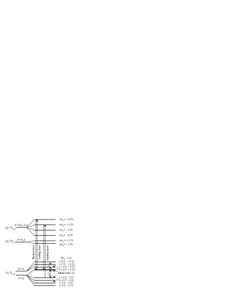
Figure 1: Energy level structure of ⁹Be⁺ at $B\approx$ 4.4609 T. $f_{\text{e}}\approx 124$ GHz, $f_{1}\approx 340$ MHz, $f_{2}\approx 288$ MHz, and $f_{3}\approx 287$ MHz. The frequency tuning of the repump laser is shown for fast repumping of the electron spin-flip transition. For the nuclear spin-flip measurements the repump laser was tuned approximately 500 MHz lower than the cooling transition.

We trapped fewer than or approximately 10³ ions in a Penning-Malmberg trap and cooled them to approximately 1 mK by Doppler laser cooling. The cooling laser also optically pumped the ions into the ($m_{I}$, $m_{J}$)=($\frac{3}{2}$, $\frac{1}{2}$) state, labeled as the initial state $|i\rangle$ in Fig. 1. [Here the states are labeled by the ($m_{I}$, $m_{J}$) quantum numbers of their largest components.] The basic experimental procedure for measuring the different transition frequencies was to (1) turn off the cooling laser, (2) probe the desired transition with the appropriate rf or microwave radiation, (3) measure the population of the ions remaining in $|i\rangle$ with the fluorescence induced by the cooling laser, (4) repump all ions to $|i\rangle$ with the cooling laser and an additional repumping laser. We used the same ions repetitively to measure all transition frequencies. We first discuss the basic experimental setup and the 124 GHz microwave system. We then discuss in more detail the measurements of the different transition frequencies and the determination of $A$ and ${g_{I}}^{\prime}/g_{J}$ at high magnetic field.

II.2 Experimental setup

II.2.1 Penning trap

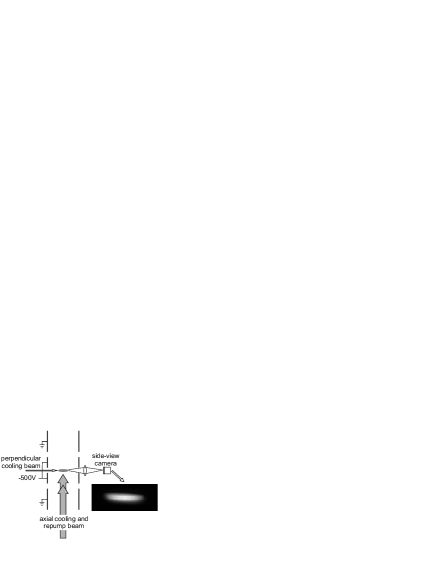
Figure 2: Schematic diagram of setup. Figure is not to scale. The trap diameter is 4 cm. The electrodes used to apply the rotating wall field are not shown. The direction of the side-view light collection and the direction of the perpendicular cooling beam form a $60^{\circ}$ angle in a plane perpendicular to the magnetic field axis. A side-view image of a plasma with approximately 500 ions is shown. The diameter of the fluorescing Be⁺ ion plasma is 400 $\mu$m. Heavier-mass impurity ions are located at larger radii than the ⁹Be⁺ ions Jensen et al. (2004).

Figure 2 shows a sketch of the Penning trap used for the high-$B$ measurements. The trap and the basic experimental setup have been described previously Huang et al. (1998); Jensen et al. (2004); Biercuk et al. (2009). The 4.4609 T magnetic field of a superconducting solenoid with a 125 mm room-temperature bore produces a ⁹Be⁺ cyclotron frequency of $\Omega_{c}=2\pi\times 7.602$ MHz. The long-term drift of the magnetic field was less than one part in $10^{9}$ per hour, resulting in an average drift of $f_{\text{e}}$ of less than 3 kHz per hour. Magnetic field shifts due to changes in the magnetic environment (due, for example, to movement of Dewars or to other activity in neighboring laboratories) were reduced by collecting data during the night. We did not stabilize the pressure in the magnet Dewar or actively cancel external magnetic field noise, which likely would have improved the long-term magnetic field stability R. S. Van Dyck et al. (1999). The field of the superconducting magnet was found to have fluctuations which were fast compared to 20 Hz, superimposed on the slow magnetic field drift and noise. The frequency spectrum of the fast fluctuations contained a continuous part and narrow peaks between 30 and 300 Hz Biercuk et al. (2009). The integrated noise of the fast fluctuations produced $\delta B/B\approx 10^{-9}$ variation in the magnetic field for measurements separated by greater than 0.1 s. The fast fluctuations contributed to the linewidth and coherence of the electron spin-flip measurement, but had no significant impact on the nuclear spin-flip measurements ($f_{1}$, $f_{2}$, and $f_{3}$). (The fast fluctuations only produce a phase modulation of a few milliradians on the nuclear spin-flip transitions.) Recent work, which will be discussed in a separate publication, indicates that the fast fluctuations are fluctuations in the homogeneous field produced by the superconducting magnet, which can be mitigated through vibration isolation of the magnet.

The Penning trap electrode structure consists of a stack of four cylindrical electrodes. The inner diameters of the cylinders are 4.1 cm and the combined length of the four cylinders is 12.7 cm. We typically operated the trap with the central cylindrical electrodes (the “ring” electrodes) biased at $-500$ V and the outer cylindrical electrodes (the “endcap” electrodes) grounded, which resulted in ⁹Be⁺ single-particle axial and magnetron frequencies of, respectively, $\omega_{z}=2\pi\times 565$ kHz and $\omega_{m}=2\pi\times 21.1$ kHz.

Due to the crossed electric and magnetic fields in a Penning trap, an ion plasma undergoes a rotation about the magnetic field axis. In thermal equilibrium this rotation is rigid Dubin and O’Neil (1999), and we use $\omega_{r}$ to denote the plasma rotation frequency. The rotation frequency $\omega_{r}$ of the ⁹Be⁺ plasma was precisely controlled with a rotating electric field (a rotating wall) Huang et al. (1998); Mitchell et al. (2001). A rotation frequency $\omega_{r}$ of 2$\pi\times$ 30 kHz or less was used, which produced planar plasmas (oblate spheroids) like that shown in Fig. 2 with ion densities of approximately 8 $\times$ 10⁷ cm^-3. The measurements presented here were obtained on small ion plasmas of fewer than 10^{3 9}Be⁺ ions. The small axial extent of the plasmas (typically less than 50 $\mu$m) reduced the effect of axial gradients in the magnetic field. Axial magnetic field gradients were shimmed to be less than two parts in 10⁸ per mm, which resulted in an axial magnetic field inhomogeneity of less than one part in 10⁹ over a 50 $\mu$m axial extent. We found no evidence for any inhomogeneous broadening of the different resonance curves discussed in Secs. II.3 and II.4.

II.2.2 Laser cooling, state preparation, and detection

Doppler laser-cooling was carried out on the 313 nm ${}^{2}S_{1/2}\ (m_{I}=\frac{3}{2},m_{J}=\frac{1}{2})$ $\rightarrow$ ${}^{2}P_{3/2}\ (m_{I}=\frac{3}{2},m_{J}=\frac{3}{2})$ transition (see Fig. 1). The 313 nm light was generated by frequency-doubling the output of a dye laser at 626 nm. The axial and perpendicular cooling beams cooled the motion parallel and perpendicular, respectively, to the magnetic-field axis Jensen et al. (2004, 2005). The axial cooling beam had a 1 mm waist diameter, a power of approximately 1 mW, and a polarization that was either linear or circular ($\sigma^{+}$). The axial cooling beam was aligned with the magnetic field axis to better than 0.01^∘. The perpendicular cooling beam was linearly polarized in a direction perpendicular to B, focused to a waist diameter of approximately 50 $\mu$m, and had a power of approximately 1 $\mu$W. A double-pass acousto-optic modulator was used to rapidly switch the cooling beams off (in less than 1 $\mu$s) before applying rf or microwave radiation to drive the desired ground-state transitions. The cooling beams were switched back on after the rf or microwave radiation was switched off.

The population of the ${}^{2}S_{1/2}\ (m_{I}=\frac{3}{2},m_{J}=\frac{1}{2})$ state (the initial state $|i\rangle$ in Fig. 1) was measured through the cooling-laser-induced resonance fluorescence. An $f/5$ imaging system was used to image the ⁹Be⁺ ion fluorescence onto the photocathode of a photon-counting imaging tube (quantum efficiency was approximately 5 %). The total imaging tube count rate was proportional to the $|i\rangle$ state population. The total photon count rate was recorded for 0.5 s both before and after applying the rf or microwave radiation. The ratio of these two count rates (with small corrections for repumping effects) measured the fraction of the ions remaining in the $|i\rangle$ state.

The cooling radiation optically pumped more than 94 % of the ions into the ${}^{2}S_{1/2}\ (\frac{3}{2},\frac{1}{2})$ state, i.e., the lower level of the cooling transition Brewer et al. (1988); Itano and Wineland (1981). This was a non-resonant optically pumping process with a time constant of approximately 5 s for the cooling laser parameters in this experiment. The repumping time on the electron spin-flip transition ($f_{\text{e}}$) was reduced to less than 1 ms by a second frequency-doubled dye laser (labeled the repump laser in Fig. 1). The repump laser was turned on after the second 0.5 s detection period (the detection period after the applied rf or microwave radiation). The $f_{1}$, $f_{2}$, and $f_{3}$ transitions involve a change in the ⁹Be⁺ nuclear spin orientation. For example, in $f_{2}$ the nuclear spin changes from $m_{I}=\frac{3}{2}$ to $m_{I}=\frac{1}{2}$. Optical repumping back to $|i\rangle$ occurred through the ${}^{2}S_{1/2}\ (\frac{1}{2},\frac{1}{2})$ $\rightarrow$ ${}^{2}P_{3/2}\ (\frac{1}{2},\frac{3}{2})$ transition and the small admixture of different ($m_{I}$, $m_{J}$) states in the $2p\,^{2}P_{3/2}$ manifold Itano and Wineland (1981). We reduced this repumping time somewhat by tuning the repump laser frequency between 400 MHz and 600 MHz below that of the cooling transition. This had the added benefit of maintaining a cold-ion plasma when most of the ions are driven to the $(m_{I}=\frac{1}{2},m_{J}=\frac{1}{2})$ state. Presumably this was because the frequency of the repump laser was now below that of the ${}^{2}S_{1/2}\ (\frac{1}{2},\frac{1}{2})$ $\rightarrow$ ${}^{2}P_{3/2}\ (\frac{1}{2},\frac{3}{2})$ transition. A similar improvement in the repumping and plasma stability was also observed for the $f_{1}$ and $f_{3}$ transitions with a “far-detuned” laser tuned 400 MHz to 600 MHz below the cooling transition. The repump or far-detuned beam was directed along the magnetic field axis of the trap, as shown in Fig. 2. The beam waist diameter was approximately 0.5 mm; the power was a few milliwatts.

II.2.3 Microwave apparatus

A sketch of the 124 GHz microwave system used to measure $f_{\text{e}}$ is shown in Fig. 3. Reference Biercuk et al. (2009) further discusses the microwave system and its use in quantum information experiments. A Gunn diode oscillator generated 30 mW of microwave power, and its frequency was coarsely set to approximately 124 GHz by a manually tuned microwave cavity. The microwave radiation was transmitted through WR-8 wave guides and launched to free space through a pyramidal rectangular microwave horn. A small fraction of the microwave power ($-10$ dB) was mixed with the 8th harmonic of a 15.5 GHz dielectric resonator oscillator (DRO). The intermediate frequency (IF) signal from the harmonic mixer was sent to a phase-locked loop (PLL) controller and phase-locked to a 76 MHz reference frequency generated by direct digital synthesis (DDS). The microwave frequency and phase were controlled by changing the frequency and phase of the DDS signal. The DDS was controlled by computer through a parallel interface. All of the frequency synthesizers used in the experiment were referenced to the same passive hydrogen maser, including the DRO and the DDS. The frequency of the passive hydrogen maser was calibrated relative to that of the NIST atomic time scale.

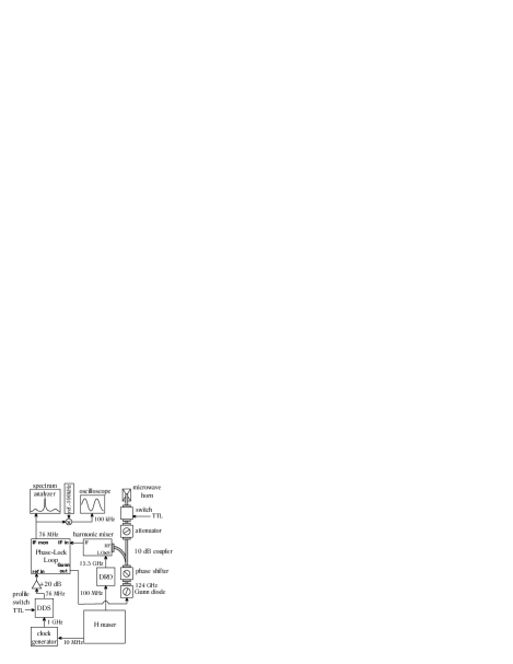
Figure 3: Schematic diagram of the 124 GHz microwave source. A Gunn diode oscillator generates 30 mW of microwave power that was transmitted through WR-8 wave guide (shown in gray) and emitted to free space via a pyramidal microwave horn. The frequency of the Gunn diode oscillator was phase-locked to a signal derived from a hydrogen-maser frequency standard.

The microwave radiation emitted from the horn was rapidly switched on and off with a reflective PIN diode switch. The ratio of the high and low power states was $26.5\pm 0.9$ dB. Switching between the high- and low-power states could cause the PLL to lose phase-lock because of the change in the reflected signal. To avoid losing phase-lock, we added a phase shifter between the Gunn diode oscillator and the PIN diode switch. (The large fringing field of the magnet made use of an isolator impractical.) The phase shifter required careful adjustment to achieve a condition where the Gunn diode oscillator would not lose lock when the microwave power was switched.

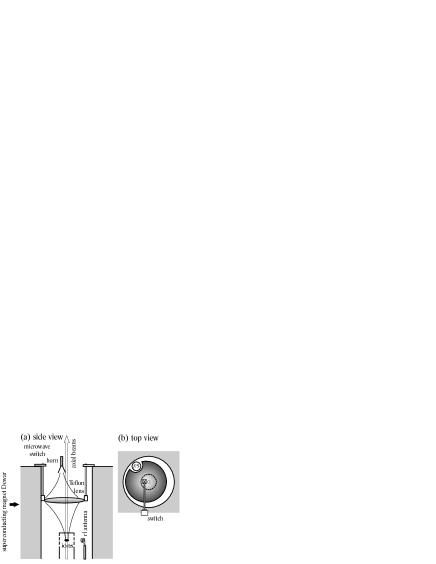
Figure 4: Schematic diagram of the quasi-optical coupling of 124 GHz microwave radiation to the ions. Figures are not to scale. (a) Side view. (b) Top view. The inner diameter of the super-conducting magnet was 12.5 cm, the distance from the horn to the lens was 29 cm, and from the lens to the ions is 28 cm. The horn was shifted off-axis in order to avoid hitting the horn with the axial laser beams. The lens was also shifted about half this amount to focus on the ions. The lens diameter was 10.2 cm. It had a cut on the side to make a room for the $f/5$ optics used for the side-view camera. Electron spin-flip $\pi$-pulse periods of 100 $\mu$s were obtained with this setup. The position of the rf antenna is also shown.

We used quasi-optical techniques (with a horn and Teflon lens) to couple the microwave radiation to the ions, as schematically shown in Fig. 4. The pyramidal horn coupled mainly to the Gaussian TEM00 mode with an initial waist diameter of approximately 0.7 cm. The waist diameter $w$ is defined by ${P(r)}/{P(0)}=e^{-2(r/w)^{2}}$, where $P(r)$ is the power per unit area at a radius $r$. The waist diameter of the Gaussian beam increases as it propagates. The beam was focused to a waist of about 0.7 cm at the ions by the hyperbolic surfaces of the lens Goldsmith (1998), which was 29 cm below the horn and 28 cm above the ions. The lens had a cut near the side for the $f/5$ side-view optics and a 4.8 mm diameter hole near center to pass laser beams (see Fig. 4). The horn was shifted off axis to avoid the laser beams, and the lens was shifted accordingly to center the microwave focus on the ions. The microwave system was on an $x$-$y$ mechanical stage, and the position of the horn was adjusted to maximize the coupling of the microwave radiation with the ions.

Electron spin-flip $\pi$-pulse periods as short as 100 $\mu$s were obtained with this microwave system. $\pi$-pulse fidelities of better than 99.9 % were measured with random benchmarking on plasmas consisting of a single plane Biercuk et al. (2009). The Ramsey free-induction decay (that is, the free-precession period in a Ramsey experiment where the fringe contrast has decayed by 1/$e$) was measured to be $T_{2}\approx 2.4$ ms, limited by the fast magnetic field fluctuations.

II.3 Electron spin-flip measurement

Figure 5 shows an electron spin-flip resonance obtained with a 600 $\mu$s square Rabi pulse. The data were fitted to the expected Rabi resonance curve Ramsey (1956),

$$P_{i}=1-\frac{(2b)^{2}}{(f_{\text{e}}-f)^{2}+(2b)^{2}}\sin\left(\pi t\sqrt{(f\text{e}-f)^{2}+(2b)^{2}}\right).$$ (4)

Here $P_{i}$ is the probability of an ion to be in state $|i\rangle$, $b\equiv\Omega/2\pi$, where $\Omega$ is the Rabi frequency, $t=600~{}\mu$s is the microwave pulse duration, $f$ is the microwave frequency, and $f_{\text{e}}$ is the electron spin-flip resonance frequency. From the fit to the data in Fig. 5, we determine a value for the electron spin-flip frequency $f_{\text{e}}=124~{}076~{}860~{}036~{}\pm 15$ Hz. The uncertainty obtained from the fit we define to be the internal error, and for electron spin-flip resonance curves taken under conditions similar to that shown in Fig. 5, the internal error was typically less than 20 Hz. Because $f_{\text{e}}$ is roughly proportional to $B$, 20 Hz corresponds to a 1.6 $\times$ 10^-10 fractional measurement of $B$, a reduction by about a factor of five, due to averaging, from the shot-to-shot variation in $B$.

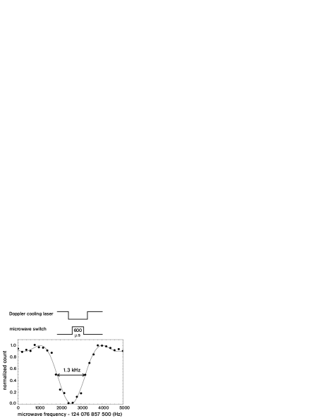
Figure 5: Electron spin-flip Rabi resonance. The microwave power is adjusted to produce a $\pi$-pulse on resonance in 600 $\mu$s. The solid line is a fit to the expected Rabi resonance, as discussed in the text. All experimental measurements were equally weighted in the fit.

The resonance curve in Fig. 5 took a few minutes to obtain. If we took many resonance curves over a longer period, the scatter in the fitted values for $f_{\text{e}}$ was larger than the internal error of an individual fit, due to slow drift and fluctuations in $B$. We define the external error to be the standard deviation of $f_{\text{e}}$, determined from many separate scans. The typical external error for data taken over a 30-minute period was greater than 40 Hz. We found the external error to be smallest between 10 PM and midnight local time. Since the measurement of $f_{\text{e}}$ was limited by the stability of $B$, reducing the internal error by narrowing the line width with longer Rabi pulses would not have benefited us.

To determine the hyperfine constant $A$, we cycled between measurements of $f_{\text{e}}$ and measurements of the nuclear spin-flip frequencies discussed in the next section. To minimize the effect of drift and slow fluctuations in $B$, it was important to complete one cycle of measurements as rapidly as conveniently possible. We found that we could complete a cycle of measurements more rapidly if we did not change the frequency of the repump laser to the repumping transition (see Fig. 1) for the $f_{\text{e}}$ measurements. Therefore, we set the frequency of the repump laser to the far-detuned position (400 MHz to 600 MHz lower than the cooling transition) for all measurements of $f_{\text{e}}$, $f_{1}$, $f_{2}$, and $f_{3}$.

II.4 Nuclear spin-flip measurements

The rf radiation used to drive the nuclear spin-flip transitions was generated by mixing the output of an 80 MHz synthesizer having 1 mHz resolution with a higher-frequency synthesizer that had lower frequency resolution. For measurements of $f_{2}$ and $f_{3}$ (approximately 290 MHz), the higher-frequency synthesizer was set to 220 MHz. For measurements of $f_{1}$ (approximately 340 MHz) the higher-frequency synthesizer was set to 280 MHz. Switching of the rf was done with a switch having approximately 90 dB isolation. The rf radiation was coupled to the ions through a two-turn rf loop antenna, placed near ions, outside the vacuum envelope (see Fig. 4).

Figure 6: $f_{2}$ resonance obtained with a 4 s Ramsey free-precession period. The rf power was adjusted to apply a $\pi$/2-pulse in 0.5 s.

Figure 6 shows an $f_{2}$ resonance curve obtained with the Ramsey method. The rf power was adjusted to achieve a $\pi/2$ pulse in 0.5 sec. The two $\pi/2$ pulses were separated by 4 s. After the Ramsey sequence, both the cooling laser and the far-detuned laser were turned on simultaneously. The power of the far-detuned beam was adjusted so that the dark state repumped with a 1/$e$ time constant of approximately 2 s. To avoid any significant ac Zeeman shifts due to the finite isolation (26 dB) of the microwave switch, the microwave frequency was detuned from resonance with $f_{\text{e}}$ by 1 MHz during the $f_{2}$ measurement. Fitting the data of Fig. 6 to a sinusoidal curve gives $f_{2}$ = 288 172 932.435 3(7) Hz. The typical external error from measurements taken over a 30 to 40 minute measurement cycle was approximately 5 mHz. A 5 mHz external error with the 6.5 kHz/mT sensitivity of this transition implies a fractional magnetic field stability of 2 $\times$ 10^-10 over a typical 30 to 40 minute period, which is comparable to what was observed on the electron spin-flip transition.

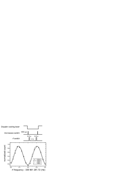
Figure 7: An $f_{1}$ resonance obtained with a 4 s Ramsey free-precession period. The rf power was adjusted to apply a $\pi$/2-pulse in 0.5 s. The microwave frequency was shifted by $\pm$100 kHz during Ramsey sequence.

Figure 7 shows an $f_{1}$ resonance curve obtained with the Ramsey method. We first transferred the population in $|i\rangle$ to the ($m_{I}=\frac{3}{2},m_{J}=-\frac{1}{2}$) state with a 600 $\mu$s $\pi$-pulse. This was followed by the Ramsey interrogation, as shown in Fig. 7. We then used a second 600 $\mu$s microwave $\pi$-pulse to transfer any ions remaining in the ($m_{I}=\frac{3}{2},m_{J}=-\frac{1}{2}$) state to $|i\rangle$. The ion population in $|i\rangle$ was then detected by the laser-induced fluorescence.

We shifted the microwave frequency by $\pm$100 kHz from resonance during the Ramsey interrogation of $f_{1}$. This prevented driving the $f_{\text{e}}$ transition with microwave radiation that leaked through the microwave switch. The DDS frequency could be switched by as much as 100 kHz, and we could still keep the Gunn diode oscillator phase-locked. A 100 kHz offset produced a 2 mHz ac Zeeman shift due to the microwave leakage through the switch. A measurement of $f_{1}$ consisted of taking two scans with alternate signs of the microwave detuning. The $f_{1}$ transition frequency was determined by fitting the average of the two scans. A fit to the data in Fig. 7 provides $f_{1}$ = 339 961 281.917 0(8) Hz. The external error from measurements taken over a 30 to 40 minute period was typically 5 mHz, about the same as for the $f_{2}$ measurements.

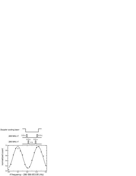
Figure 8: An $f_{3}$ resonance obtained with the Ramsey method. The power of the rf was adjusted to apply a $\pi$/2-pulse in 0.5 second.

Figure 8 shows an $f_{3}$ resonance curve obtained with a 4 s Ramsey free-precession period. The pulse sequence was very similar to the one for $f_{1}$. The microwave $\pi$-pulse in the $f_{1}$ measurement was replaced with a 0.5 s rf $\pi$-pulse to transfer the population from $|i\rangle$ to the $(m_{I}=\frac{1}{2},m_{J}=\frac{1}{2})$ state. Then the rf frequency and amplitude were changed, and we applied a Ramsey sequence with a 4 s free-precession period. The frequency of the microwave radiation was detuned from resonance by 1 MHz during the $f_{3}$ measurement. A fit to the data in Fig. 8 gives $f_{3}$ = 286 586 654.158 5(14) Hz.

The length of the Ramsey free-precession periods in the nuclear spin-flip measurements (4 s) was limited by the heating, presumably due to collisions with residual gas molecules, that occurred when the cooling laser was turned off Jensen et al. (2004). For free precession periods longer than 4 s, the ion fluorescence decreased, due to the increase in the Doppler width of the cooling transition. This added noise and complicated the signal analysis. Longer free-precession periods (20 s to 100 s) have been used with sympathetic cooling in previous low-$B$ measurements Bollinger et al. (1989, 1991). The nuclear spin-flip measurements at 4.4609 T were limited by magnetic-field instabilities, so there was no compelling reason to use longer free-precession periods.

II.5 Experimental results

To determine the hyperfine constant $A$, resonance curves such as those shown in Figs. 5–7 were taken in succession, as shown in Fig. 9, and fits to the resonance curves were used to determine $f_{\text{e}}$, $f_{1}$, and $f_{2}$. A typical measurement cycle consisted of an $f_{\text{e}}$ measurement, followed by an $f_{1}$ measurement, followed by another $f_{\text{e}}$ measurement, followed by an $f_{2}$ measurement, followed by a final $f_{\text{e}}$ measurement. One measurement cycle took 30 to 40 minutes to complete. The average of the three $f_{\text{e}}$ measurements in one cycle was use to determine $f_{\text{e}}$. The uncertainty in $f_{\text{e}}$ was taken to be the external error from the scatter in the three measurements, which was typically about 40 Hz. The uncertainties assigned to $f_{1}$ and $f_{2}$ were the external errors from the scatter in the $f_{1}$ and $f_{2}$ measurements from consecutive measurement cycles, which was typically about 5 mHz.

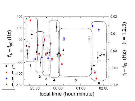
Figure 9: (Color online) Summary of measurements taken during a 4 hour run at night. The measured electron and nuclear spin-flip frequencies (relative to fixed frequencies $f_{{\text{e}}0}=124\,076\,861\,270$ Hz, $f_{10}=339\,961\,281.922$ Hz, $f_{20}=288\,172\,932.440$ Hz, and $f_{30}=286\,586\,654.160$ Hz) are plotted against the time the measurement was made. The measurements are grouped into cycles, labeled 1–6 on the graph. Each cycle was used to determine a value of $A$ and ${g_{I}}^{\prime}/g_{J}$. The error bars are the internal errors obtained from the fits to the resonance curves. Due to magnetic field drift, $f_{\text{e}}$ drifted down by about 100 Hz during this run. This is consistent with the drifts observed with $f_{1}$ and $f_{2}$, where $f_{1}$ decreases and $f_{2}$ increases with decreasing magnetic field.

All known systematic errors in the nuclear spin-flip resonance frequency measurements, other than those due to the magnetic field instability, were less than 1 mHz. The largest systematic error is due to microwave radiation leaking through the microwave switch. As discussed in Sec. II.4, this produced a 2 mHz shift in the $f_{1}$ resonance curve. However, by taking data with the microwave frequency shifted off resonance by both $+100$ kHz and $-100$ kHz, this shift could effectively be canceled. During a 4 s nuclear spin-flip measurement, the ion temperature increased due to collisions with the room temperature residual background gas. Previous studies indicated that the temperature increase over a 4 s period is limited to a few kelvins Jensen et al. (2004, 2005). However even a 10 K temperature would produce only an approximately $-0.1$ mHz time-dilation shift in the measured ⁹Be⁺ nuclear spin-flip frequency. We performed some simple checks for unknown systematic errors by varying the length of the Rabi pulse in the $f_{\text{e}}$ measurement and the length of the free-precession period in the nuclear spin-flip measurements. In addition, we took some $f_{1}$ and $f_{2}$ measurements with an 8 s Rabi pulse. No systematic dependencies were observed at the level permitted by the magnetic field stability.

For each measurement cycle, the Breit-Rabi formula [Eq. (2)] was used to solve for values of $A$, ${g_{I}}^{\prime}/g_{J}$, and $X$. The uncertainties in these values were determined by using the Breit-Rabi formula to solve again for $A$, ${g_{I}}^{\prime}/g_{J}$, and $X$, but with $f_{\text{e}}$, $f_{1}$, and $f_{2}$ set to the limits of their uncertainties. We conservatively assigned the largest uncertainty that could be obtained from the different combinations of limits. For example, if $\delta f_{\text{e}}$, $\delta f_{1}$, and $\delta f_{2}$ are the uncertainties in $f_{\text{e}}$, $f_{1}$, and $f_{2}$, solving the Breit-Rabi formula with the frequency values $f_{\text{e}}+\delta f_{\text{e}}$, $f_{1}+\delta f_{1}$, and $f_{2}+\delta f_{2}$ gives the largest uncertainty for $A$, while solving the Breit-Rabi formula with the frequency values $f_{\text{e}}+\delta f_{\text{e}}$, $f_{1}-\delta f_{1}$, and $f_{2}+\delta f_{2}$ gives the largest uncertainty for ${g_{I}}^{\prime}/g_{J}$.

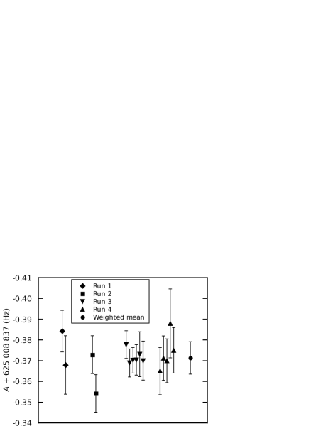
Figure 10: Summary of the measurements of the high-field hyperfine constant $A$. Each of the four runs is a series of determinations of $A$ made on the same date. Each $A$ value is determined from the Breit-Rabi formula and one cycle of $f_{\text{e}}$, $f_{1}$, and $f_{2}$ measurements. The assignment of uncertainties is described in the text.

Figure 10 summarizes the measurements of $A$ at high magnetic field. Four different sets of data were taken on four different dates over a period of two months. Each set of data consisted of at least two and as many as six measurement cycles. The consistency of the data is good. The standard deviation from the scatter of the 15 different measurements of $A$ is 7 mHz, which is slightly less than the average 11 mHz uncertainty of an individual measurement. For the determination of $A$ we use a weighted average of the data shown in Fig. 10 and conservatively assign an 11 mHz uncertainty, the average uncertainty for a single measurement cycle. An 11 mHz uncertainty corresponds to about a $3\times 10^{-10}$ fractional magnetic field instability, about a factor of three below the shot-to-shot fluctuations in the magnetic field. We believe that an assignment of a smaller uncertainty would require a careful study of the statistics of the magnetic field fluctuations. The result is

$$A(4.4609~{}\text{T})=-625\,008\,837.371(11)~{}\text{Hz}.$$ (5)

Although $A$ was the main focus of this study, a value of the $g$-factor ratio is also obtained from the same analysis:

$${g_{I}}^{\prime}/g_{J}=2.134\,779\,852\,7(10)\times 10^{-4}.$$ (6)

In four of the data cycles shown in Fig. 10, the fourth frequency $f_{3}$ was measured in addition to $f_{\text{e}}$, $f_{1}$, and $f_{2}$. These measurements were used to place upper limits on corrections to the Breit-Rabi formula at a fixed value of $B$. The results are listed in Table 1. If the Breit-Rabi formula is assumed to be correct, and $A$ and ${g_{I}}^{\prime}/g_{J}$ are fixed at the values given by the complete set of 15 data cycles [Eqs. (5) and (6)], then any of the three frequencies $f_{\text{e}}$, $f_{1}$, or $f_{2}$ can be be used to determine $X$ for a given data cycle. This value of $X$ can then be used to predict $f_{3}$ for that data cycle. In practice $f_{2}$ tended to yield the most consistent values of $X$. The rms difference between the measured value of $f_{3}$ and the value predicted from the measurement of $f_{2}$ was 7 mHz. This is consistent with the noise expected from magnetic field fluctuations. We use these results to place an upper limit of 10 mHz on any shifts of $f_{3}$ at $B$ = 4.4609 T due to corrections to the Breit-Rabi formula. More specifically, we can set limits on corrections to the Breit-Rabi formula having the form of the quadrupole diamagnetic shift or of the hyperfine-assisted Zeeman shift. Since all of the measurements were made at nearly the same value of $B$, this test is not sensitive to modifications to the Breit-Rabi formula that amount to a dependence of either $A$ or ${g_{I}}^{\prime}/g_{J}$ on $B$.

Table 1: Measured values of $f_{3}$ and values of $f_{3}$ predicted from the Breit-Rabi formula. All frequencies are in hertz.

$f_{2}$ (measured)	$f_{3}$ (predicted from $f_{2}$)	$f_{3}$ (measured)	$f_{3}$ (predicted) $-$ $f_{3}$ (measured)
288 172 931.651 0	286 586 653.404 9	286 586 653.400 3	0.0046
288 172 931.609 7	286 586 653.365 8	286 586 653.372 7	-0.0069
288 172 932.447 0	286 586 654.156 8	286 586 654.167 1	-0.0103
288 172 932.453 5	286 586 654.162 9	286 586 654.157 8	0.0051

The energy shift of an $(m_{I},m_{J})$ state due to the quadrupole diamagnetic shift, at a fixed value of $B$, has the form Lipson et al. (1986)

$$E_{Q}=hf_{Q}B^{2}\frac{[I(I+1)-3m_{I}^{2}]}{I(2I-1)}.$$ (7)

If the only correction to the Breit-Rabi formula is given by Eq. (7), then agreement of the measured and predicted values of $f_{3}$ to less than 10 mHz sets a limit $|f_{Q}|B^{2}<5$ mHz at $B$ = 4.4609 T, or $|f_{Q}|<2.5\times 10^{-4}$ Hz T^-2.

The hyperfine-assisted Zeeman shift of an $(m_{I},m_{J})$ state has the form Fortson (1987)

$$E_{\text{HZ}}=2h\beta_{\text{HZ}}B[m_{I}^{2}m_{J}-I(I+1)m_{J}+m_{I}/2].$$ (8)

If the only correction to the Breit-Rabi formula is given by Eq. (8), then agreement of the measured and predicted values of $f_{3}$ to $\pm 10$ mHz sets a limit $|2\beta_{\text{HZ}}B|<6.7$ mHz at $B$ = 4.4609 T, or $|\beta_{\text{HZ}}|<7.5\times 10^{-4}$ Hz T^-1.

III Determination of $\bm{k}$ from high-field measurements and previous low-field measurements

The present experimental results can be combined with previous measurements made by some of the present authors at lower values of $B$ to determine the $B$-dependence of $A$ or ${g_{I}}^{\prime}/g_{J}$. Preliminary values of $A$ and ${g_{I}}^{\prime}/g_{J}$ were given in Ref. Wineland et al. (1983) but not the transition frequencies on which they were based. We now supplement Ref. Wineland et al. (1983) with the transition frequencies and a final determination of $A$ and ${g_{I}}^{\prime}/g_{J}$. Two nuclear spin-flip frequencies, labeled 1 and 3 in Table 2, were measured near two particular values of $B$ where the first derivatives of the frequencies are zero. Electron spin-flip frequencies, labeled 2 and 4 in Table 2, were measured at the same two values of $B$. The experimental methods have been described in detail Wineland et al. (1983); Bollinger et al. (1985, 1989, 1991). Transition 3 is known better than transition 1 because it was studied for use as a frequency standard Bollinger et al. (1985, 1991). The value we report for transition 3 in Table 2 is slightly different than that reported in Bollinger et al. (1985) because it includes additional measurements made in 1988 and 1989 as well as an evaluation of the background pressure shift.

If no account is taken of any $B$-dependence of $A$ or ${g_{I}}^{\prime}/g_{J}$, the four frequency measurements, together with the Breit-Rabi formula, yield a system of four equations with four unknowns, $A$, ${g_{I}}^{\prime}/g_{J}$, $X_{1}$, and $X_{2}$, where $X_{1}$ is the value of $X$ for transitions 1 and 2, and $X_{2}$ is the value of $X$ for transitions 3 and 4. The frequencies given in Table 2 yield $A=-625\,008\,837.053(11)$ Hz and ${g_{I}}^{\prime}/g_{J}=2.134\,779\,851\,8(23)\times 10^{-4}$. The precise values of $X_{1}$ and $X_{2}$ are not important, since they reflect only the value of $B$ at which the experiment was performed, not any intrinsic property of the ⁹Be⁺ ion. Comparing these results to Eqs. (5) and (6), we see that there is clear evidence for $B$-dependence of $A$, but that ${g_{I}}^{\prime}/g_{J}$ is independent of $B$ to within experimental error.

Table 2: Low-$B$ resonance frequencies used to determine $A$ and ${g_{I}}^{\prime}/g_{J}$.

Label	$(m_{I},m_{J})\leftrightarrow({m_{I}}^{\prime},{m_{J}}^{\prime})$	$B$(T)	Frequency (Hz)	Uncertainty (Hz)
1	$(\frac{1}{2},-\frac{1}{2})\leftrightarrow(\frac{3}{2},-\frac{1}{2})$	0.677395	321 168 429.685	0.010
2	$(\frac{3}{2},-\frac{1}{2})\leftrightarrow(\frac{3}{2},\frac{1}{2})$	0.677395	18 061 876 000	150 000
3	$(-\frac{1}{2},\frac{1}{2})\leftrightarrow(-\frac{3}{2},\frac{1}{2})$	0.819439	303 016 377.265 20	0.000 11
4	$(-\frac{3}{2},-\frac{1}{2})\leftrightarrow(-\frac{3}{2},\frac{1}{2})$	0.819439	23 914 008 800	150 000

From theoretical considerations and from experimental results with Rb, a quadratic $B$-dependence of $A$ is expected. If we assume that $A(B)=A_{0}\times(1+kB^{2})$, then there are five unknowns to solve for: $A_{0}$, $k$, ${g_{I}}^{\prime}/g_{J}$, $X_{1}$, and $X_{2}$. In addition to the four equations for the low magnetic field measurements, derived from the Breit-Rabi formula, a fifth equation is given by the expression for the high-$B$ value of $A$:

$$A_{0}\times(1+k{B_{3}}^{2})=-625\,008\,837.371~{}\text{Hz},$$ (9)

where $B_{3}=4.4609$ T. Solving the set of five equations gives

$$A_{0} = -625\,008\,837.044(12)~{}\text{Hz},$$ (10a)

$$k = 2.63(18)\times 10^{-11}\;\text{T}^{-2},$$ (10b)

$${g_{I}}^{\prime}/g_{J} = 2.134\,779\,852\,0(23)\times 10^{-4}.$$ (10c)

The uncertainties of the parameters are obtained by varying the experimental frequencies through their uncertainties. The value of ${g_{I}}^{\prime}/g_{J}$ given by Eq. (10c) is consistent with, but less precise than, that obtained from the high-$B$ data alone [Eq. (6)].

IV Calculation of diamagnetic hyperfine shift coefficient $\bm{k}$

In nonrelativistic atomic theory, the diamagnetic shift in hyperfine structure arises as a cross term involving both the diamagnetic interaction and the hyperfine interaction in second-order perturbation theory. Let the unperturbed Hamiltonian for an $N$-electron atom with nuclear charge $Ze$ be

$$H_{0}=\sum_{i=1}^{N}\frac{\textbf{p}_{i}^{2}}{2m}-\sum_{i=1}^{N}\frac{Ze^{2}}{4\pi\epsilon_{0}r_{i}}+\sum_{i<j}\frac{e^{2}}{4\pi\epsilon_{0}|\textbf{r}_{i}-\textbf{r}_{j}|},$$ (11)

where $m$ is the electron mass, $-e$ is the electron charge, and $\textbf{r}_{i}$ and $\textbf{p}_{i}$ are the position and momentum of the $i$th electron. The interaction with an external magnetic field $\textbf{B}=B\hat{\textbf{z}}$ is taken into account by the minimal coupling prescription, i.e., making the replacement $\textbf{p}_{i}\rightarrow\textbf{p}_{i}+e\textbf{A}(\textbf{r}_{i})$, where A is the vector potential function, $\bm{\nabla}\times\textbf{A}=\textbf{B}$. Nuclear Zeeman, electron spin Zeeman, and hyperfine interactions are also added as perturbations to $H_{0}$. The kinetic energy term for the $i$th electron in Eq. (11) undergoes the change

$$\frac{\textbf{p}_{i}^{2}}{2m} \rightarrow \frac{[\textbf{p}_{i}+e\textbf{A}(\textbf{r}_{i})]^{2}}{2m}$$ (12b)

$$= \frac{\textbf{p}_{i}^{2}}{2m}+\frac{e[\textbf{p}_{i}\cdot\textbf{A}(\textbf{r}_{i})+\textbf{A}(\textbf{r}_{i})\cdot\textbf{p}_{i}]}{2m}$$

$$+\frac{e^{2}\textbf{A}^{2}(\textbf{r}_{i})}{2m}$$

$$= \frac{\textbf{p}_{i}^{2}}{2m}+H_{i}^{\text{p}}+H_{i}^{\text{d}}.$$ (12c)

The term containing the first power of A is called the paramagnetic interaction $H_{i}^{\text{p}}$, while the one containing $\textbf{A}^{2}$ is called the diamagnetic interaction $H_{i}^{\text{d}}$. The division into paramagnetic and diamagnetic parts is gauge-dependent, but the choice of gauge,

$$\textbf{A}(\textbf{r})=\frac{1}{2}\textbf{r}\times\textbf{B},$$ (13)

is particularly convenient. With that choice, the paramagnetic term becomes

$$H_{i}^{\text{p}} = \frac{e}{2m}[\textbf{p}_{i}\cdot\textbf{A}(\textbf{r}_{i})+\textbf{A}(\textbf{r}_{i})\cdot\textbf{p}_{i}]$$ (14a)

$$= \frac{e}{4m}(\textbf{p}_{i}\cdot\textbf{r}_{i}\times\textbf{B}+\textbf{r}_{i}\times\textbf{B}\cdot\textbf{p}_{i})$$ (14b)

$$= \frac{e}{2m}\textbf{r}_{i}\times\textbf{p}_{i}\cdot\textbf{B}=\frac{e}{2m}\bm{\ell}_{i}\cdot\textbf{B}=\frac{e(\ell_{i})_{z}B}{2m},$$ (14c)

where $\bm{\ell}_{i}=\textbf{r}_{i}\times\textbf{p}_{i}$ is the orbital angular momentum of the $i$th electron. The diamagnetic term becomes

$$H_{i}^{\text{d}}=\frac{e^{2}\textbf{A}^{2}(\textbf{r}_{i})}{2m}=\frac{e^{2}}{8m}(\textbf{r}_{i}\times\textbf{B})^{2}=\frac{e^{2}}{8m}(x_{i}^{2}+y_{i}^{2})B^{2}.$$ (15)

$H_{i}^{\text{d}}$ can be divided into a spherically symmetric (scalar) part and a rank-2 spherical tensor part:

$$H_{i}^{\text{d}}=\frac{e^{2}B^{2}r_{i}^{2}}{12m}+\frac{e^{2}B^{2}r_{i}^{2}}{24m}(1-3\cos^{2}\theta_{i})\equiv H_{i}^{\text{d}0}+H_{i}^{\text{d}2}.$$ (16)

The total paramagnetic interaction is obtained by summing $H_{i}^{\text{p}}$ over all electrons:

$$H^{\text{p}}=\sum_{i=1}^{N}H_{i}^{\text{p}}=\frac{eB}{2m}\sum_{i=1}^{N}(\ell_{i})_{z}=\frac{eB}{2m}L_{z},$$ (17)

where $L_{z}$ is the $z$-component of the total electronic orbital angular momentum. To a very good approximation, the ground electronic state is an $S$-state, that is, an eigenstate of $\textbf{L}^{2}$ with $L=0$, so $H^{\text{p}}$ can be neglected.

The total scalar part of the diamagnetic interaction is

$$H^{\text{d}0}=\sum_{i=1}^{N}H_{i}^{\text{d}0}=\sum_{i=1}^{N}\frac{e^{2}B^{2}r_{i}^{2}}{12m}.$$ (18)

In first-order perturbation theory, this leads to a common shift of all of the hyperfine-Zeeman sublevels of the ground electronic state. In second-order perturbation theory, there is a cross term that is first-order in both $H^{\text{d}0}$ and the Fermi contact hyperfine interaction. This leads to an effective interaction that appears as a shift in the hyperfine $A$ value, proportional to $B^{2}$ Bender (1964); Larson (1978); Economou et al. (1977); Ray et al. (1979); S. J. Lipson (1986). Evaluation of the second-order perturbation term yields the constant $k$.

Unpublished calculations by Lipson, similar to those done for Rb Lipson et al. (1986); S. J. Lipson (1986), yielded $k=2.52\times 10^{-11}$ T^-2 for Be⁺. These calculations used Hartree-Fock-Slater wave functions Herman and Skillman (1963). The inclusion of all intermediate states, including the continuum, was done by solving an inhomogeneous differential equation for the perturbed wave function Sternheimer (1951); Dalgarno and Lewis (1955). Similar calculations were done by one of the present authors (W.M.I.), but using a parametric potential for Be⁺ that reproduces the experimental energy levels Ganas (1979). This yielded $k=2.68\times 10^{-11}$ T^-2. The estimate given in Ref. Wineland et al. (1983) of $\Delta A=-0.017$ Hz T^-2 (equivalent to $k=2.7\times 10^{-11}$ T^-2) was based on these calculations.

Another method of obtaining $k$ to the same order in perturbation theory is to calculate an approximate electronic wave function that is accurate to first order in $H^{\text{d}0}$ and then to calculate the mean value of the hyperfine interaction with these wave functions. A simple way to do this is to use the MCHF (multiconfiguration Hartree-Fock) or MCDHF (multiconfiguration Dirac-Hartree-Fock) method, where an additional term, $br_{i}^{2}$ is added to each single-electron Hamiltonian. Unlike model potential methods, MCHF and MCDHF are ab initio in the sense that they require no experimental input, such as observed energy levels, only values of fundamental constants.

The GRASP set of MCDHF programs Grant (2007); Parpia et al. (1996); Jönsson et al. (1996, 2007) were used to calculate correlated wave functions for Be⁺ with and without the $br_{i}^{2}$ term and to calculate hyperfine constants with these wave functions Itano et al. (2009). The calculation of the unperturbed hyperfine constant $A_{0}$ for ⁹Be⁺ was similar to that done by Bieroń et al., Bieroń et al. (1999) but less extensive, leaving out for example nuclear recoil and the Breit interaction. The result, $A_{0}=-624.19$ MHz, is within 0.13 % of the experimental value. The calculation was then modified by including the $br_{i}^{2}$ terms in the Hamiltonian. In Hartree atomic units ($e=m=\hbar=1$), $b$ is dimensionless. It was varied from $1\times 10^{-5}$ to $2\times 10^{-3}$. The change in $A$, relative to $A_{0}$, was found to be proportional to $b$ for $b\leq 1\times 10^{-4}$. Evaluating the constant of proportionality yields $k=2.645(2)\times 10^{-11}$ T^-2, where the uncertainty here reflects only numerical error, not error due to physical approximations, such as neglect of the Breit interaction. However, given the good agreement of the calculated and experimental values of $A_{0}$, we estimate the error of the calculated value of $k$ to be no more than 1 %. All of the calculated values of $k$, including Hartree-Fock-Slater, parametric potential, and MCDHF, are in good agreement with the experimental result within the experimental error of 7 %.

The use of the diamagnetic potential in a relativistic calculation requires some justification, since the minimal coupling prescription does not yield a term proportional to $\textbf{A}^{2}$ in the Dirac Hamiltonian Luber et al. (2009). Instead of Eq. (12b) we have, for the kinetic energy term in the single-electron Dirac Hamiltonian:

$$c\bm{\alpha}\cdot\textbf{p}_{i}\rightarrow c\bm{\alpha}\cdot[\textbf{p}_{i}+e\textbf{A}(\textbf{r}_{i})]=c\bm{\alpha}\cdot\textbf{p}_{i}+ec\bm{\alpha}\cdot\textbf{A}(\textbf{r}_{i}),$$ (19)

where

$$\bm{\alpha}=\left(\begin{array}[]{cc}0&\bm{\sigma}\\ \bm{\sigma}&0\end{array}\right),$$ (20)

and $\bm{\sigma}=(\sigma^{1},\sigma^{2},\sigma^{3})$ is defined in terms of the Pauli matrices $\sigma^{i}$. Since the field-dependent perturbation only contains $B$ to the first power, calculation of $k$ with Eq. (19) requires third-order perturbation theory (two orders in the magnetic field interaction and one order in the hyperfine interaction), unlike the nonrelativistic case, which requires only second-order perturbation theory.

Kutzelnigg Kutzelnigg (2003) showed that a unitary transformation of the Dirac Hamiltonian in the presence of a magnetic field yields terms resembling the nonrelativistic paramagnetic and diamagnetic terms, plus another term which is first-order in A and whose effect goes to zero in the nonrelativistic limit. This justifies the use of second-order perturbation theory to calculate $k$ in the relativistic case. The relativistic form of the single-electron diamagnetic interaction is Kutzelnigg (2003); Luber et al. (2009)

$${H_{i}^{\text{d}}}(\text{rel})=\beta\frac{e^{2}\textbf{A}^{2}(\textbf{r}_{i})}{2m},$$ (21)

which differs from the nonrelativistic form [Eq. (15)] only by the factor of $\beta$, where $\beta$ is the $4\times 4$ matrix

$$\beta=\left(\begin{array}[]{cc}I&0\\ 0&-I\end{array}\right),$$ (22)

where $I$ is a $2\times 2$ identity matrix. The factor of $\beta$ was found also by Szmytkowski by a different method Szmytkowski (2002). The effect of $\beta$ on a matrix element of ${H_{i}^{\text{d}}}(\text{rel})$ is to reverse the sign of the integral involving the product of the small components of the Dirac orbitals. Thus, the relative error incurred by ignoring $\beta$ should be less than $(Z\alpha)^{2}$, where $\alpha$ here is the fine-structure constant $e^{2}/(4\pi\epsilon_{0}\hbar c)$. This error can be neglected for Be⁺ ($Z=4$) but may amount to a few percent for Rb ($Z=37$).

The total tensor part of the nonrelativistic diamagnetic interaction is

$$H^{\text{d}2}=\sum_{i=1}^{N}H_{i}^{\text{d}2}=\sum_{i=1}^{N}\frac{e^{2}B^{2}r_{i}^{2}}{24m}(1-3\cos^{2}\theta_{i}).$$ (23)

In first-order perturbation theory, this leads to no energy shifts in the ground electronic state. In second-order perturbation theory, there is a cross term that is first-order in both $H^{\text{d}2}$ and the electric quadrupole hyperfine interaction. This leads to an effective interaction called the magnetically induced quadrupole hyperfine interaction Lipson et al. (1986); S. J. Lipson (1986). Comparison of the second-order perturbation expression for the induced quadrupole interaction and the expression for the quadrupole antishielding factor $\gamma_{\infty}$ defined by Sternheimer L. Armstrong, Jr. (1971) yields

$$f_{Q}=\frac{e^{2}Q\gamma_{\infty}}{24mh},$$ (24)

where $f_{Q}$ is the coefficient of the induced quadrupole interaction defined in Eq. (7). This form is useful because values of $\gamma_{\infty}$ have already been calculated for many atoms and ions. The value $\gamma_{\infty}=0.7088$ for Be⁺ has been calculated in a Hartree-Fock approximation Langhoff and Hurst (1965). The most recent experimental value of the ⁹Be nuclear quadrupole moment is $5.288(38)\times 10^{-30}$ m² Pyykkö (2008). These values of the constants yield the estimate $f_{Q}=6.64\times 10^{-6}$  Hz T^-2, which is much smaller than the experimental upper limit set in Sec. II.5.

The hyperfine-assisted Zeeman shift can be estimated by the same method as that used for the rubidium atom Fortson (1987). In this approximation, the hyperfine matrix elements are given by the Fermi-Segrè formula Fermi and Segrè (1933), the $ns$-state energies are obtained from a hydrogenic (quantum defect) approximation, and the continuum $s$-state wave functions are obtained from a Coulomb approximation. In this approximation, the coefficient $\beta_{\text{HZ}}$ for ⁹Be⁺ is equal to $2.61\times 10^{-4}$ Hz T^-1, which is smaller than the experimental upper limit set in Sec. II.5.

Some other $B$-dependent shifts are in principle present, such as a magnetic-field-induced spin-dipole hyperfine term, but based on calculations done for Rb S. J. Lipson (1986) they are likely to be much smaller than the terms already considered. Various corrections to $g_{J}$ and to ${g_{I}}^{\prime}$ (e.g., nuclear diamagnetic shielding) are calculable but are beyond the scope of this paper. For recent calculations of $g_{J}$ for Be⁺ and other three-electron atoms, see Refs. Yan (2001, 2002); Glazov et al. (2004); Moskovkin et al. (2008). For a recent calculation of the nuclear diamagnetic shielding of Be⁺, see Ref. Pachucki and Puchalski (2010).