Rotating Bose-Einstein condensate in an square optical lattice: vortex configuration for ground state in Josephson junction arrays regime

Abstract

We consider a rotating Bose-Einstein condensate in a square optical lattice in the regime in which the Hamiltonian of the system can be mapped onto a Josephson junction array. In an approximate scheme where the couplings are assumed uniform, the ground state energy is formulated in terms of the vortex configuration. The results are compared with experimental results and also previously reported results for frustrated XY model. We also show that vortex configuration is robust with respect to change of couplings and therefore the results remain valid when we consider more realistic model with non-uniform couplings.

1 Introduction

After the experimental realization of Bose-Einstein condensation (BEC)[1], it becomes an interesting topic in science[2, 3, 4, 5]. This physical system has close relation with other important physical problems in condense matter, e.g. Bloch Oscillations[6, 7, 8, 9], Wannier-Stark Ladders[10], Josephson junction arrays[11, 12, 13, 14, 15, 16, 17] and superfluid to the Mott-insulator transition[18, 19, 20, 21, 22].

Behavior of a rotating BEC in an optical lattice is similar to that of a Superconductor in the magnetic field [23, 24, 25]. When there is just trap potential without the lattice structure, the Abrikasov vortex lattice can be observed just like type II Superconductors[11, 12, 14, 15, 26, 27, 28, 29, 30, 31]. When the lattice structure is added to system, the question of the vortex lattice in ground state becomes more complicated[32]. There are many experimental studies on this system with optical lattices of different symmetries, specially with square lattice[33, 34, 35]. With some criteria this problem can be mapped to problem Josephson Junction arrays (JJAs) and numerical experiments show that vortex lattice is same for both the systems[12, 14].

We focus on study of problem in this regime and extend our previous results[36] for an optical lattice with square symmetry. We calculate vortex configuration for few rational rotation numbers and show that there is good agreement with experimental results on rotating BEC and reported result for Josephson junctions lattices[37].

Structure of paper is as follows: In section II we formulate problem in JJA regime. In section III we focus on vortex lattice with rational rotation numbers and compare our result with previous experimental and numerical results. In the last section main results are highlighted and suggestions for future works have been given.

2 Rotating BEC in an optical lattice

Hamiltonian for a BEC in an optical lattice with a rotation frequency $\Omega\hat{z}$ is,

$$\hat{H}=\int dr\hat{\Psi}^{\dagger}[\frac{(-i\hbar\nabla-M\Omega\hat{z}\times r)}{2M}+V_{ext}+\frac{g}{2}\hat{\Psi}^{\dagger}\hat{\Psi}-\mu]\hat{\Psi}$$ (1)

where $M$ is the atomic mass and $g=4\pi\hbar^{2}a/M$ the coupling constant with the $s$-wave scattering length $a$. Conservation of the total number of particles is ensured by chemical potential $\mu$. The external potential $V_{ext}=V_{h}+V_{O}$ consists of two parts: modified harmonic potential $V_{h}=M(\omega_{\perp}^{2}-\Omega^{2})r^{2}/2+M\omega_{z}^{2}z^{2}/2$ and the potential of the optical lattice $V_{O}$, which may be chosen as periodic[38], quasiperiodic[38, 39], or random[40]. For example, the potential with square symmetry can be written as $V_{O}=V_{0}[sin^{2}(kx)+sin^{2}(ky)]$, with the periodicity $\pi/k$.

For a large $\omega_{z}$, we can suppose that the system is frozen in the axial direction. If the energy due to the interaction and the rotation is small compared to the energy separation between the lowest and the first excited band, the particles are confined to the lowest Wannier orbitals[14]. Therefore We can write $\psi$ in the Wannier basis as

$$\hat{\Psi}(r)=\sum_{i=1}^{N}\hat{a}_{i}w_{i}(r)exp(\frac{im}{\hbar}\int_{r_{i}}^{r}A(r^{\prime}).dr^{\prime}),$$ (2)

where $A=\Omega\hat{z}\times r$ is the analog of the magnetic vector potential, $w_{j}(r)=w(r-r_{i})$ the normalized Wannier wave-function localized in the $i$-th well and $\hat{m}_{i}=\hat{a}_{i}^{{\dagger}}\hat{a}_{i}$ the number operator. Substituting 2 in the Hamiltonian 1 leads to the Bose-Hubbard model in the rotating frame:

$$\hat{H} = -t\sum_{<i,j>}(\hat{a}^{{\dagger}}_{i}\hat{a}_{j}e^{-A_{ij}}+h.c.)$$ (3)

$$+ \sum_{i}(\epsilon_{i}-\mu)\hat{m}_{i}+\frac{U}{2}\sum_{i}\hat{m}_{i}(\hat{m}_{i}-1),$$

where $\langle i,j\rangle$ means $i$ and $j$ are nearest neighbors, $t\approx-\int drw_{j}^{*}(-\hbar^{2}\nabla^{2}/2m+V_{O})w_{j}$ is the hopping matrix element, $\epsilon_{i}=\int drw^{*}_{i}V_{h}w_{i}$ an energy offset of each lattice site and $U=g\int dr|w_{i}|^{4}$ the on-site energy. The rotation effect is described by $A_{ij}$ proportional to the line integral of $A$ between the $i$-th and $j$-th sites: $A_{ij}=(m/\hbar)\int_{r_{i}}^{r_{j}}A(r^{\prime}).dr^{\prime}$.

If the number of atoms per site is large ($n_{i}\gg 1$), the operator can be expressed in terms of its amplitude and phase, and the amplitude by the $c$-number as $\hat{a_{i}}\approx\sqrt{m_{i}}e^{i\hat{\theta}_{i}}$. Using $\hat{m}_{i}=m_{i}-i\partial/\partial\theta_{i}$ and $\hat{\theta}_{i}=\theta_{i}$, Eq. 3 reduces to the quantum phase model:

$$\hat{H}=-\sum_{<i,j>}J_{ij}cos(\theta_{i}-\theta_{j}+A_{ij})-\frac{U}{2}\sum_{i}\frac{\partial^{2}}{\partial\theta_{i}^{2}},$$ (4)

where $J_{ij}=2t\sqrt{m_{i}m_{j}}$. Also, the atoms are assumed to be distributed such as they satisfy the condition $\epsilon_{i}+Un_{i}=\mu$. The magnitude of $J_{ij}$ decreases from the central sites outward since $m_{i}$ has the profile of an inverted parabola as we can see from solution of 1D case in Fig. 1.

Figure 1: Solution of GP equation for a periodic one dimensional potential. It can be seen that $|\Psi|^{2}$ is enveloped by an inverted parabola shape.

Eq. 2.4 is just the Hamiltonian of a lattice of small Josephson junctions with inhomogeneous coupling constants $J_{ij}$. With $J_{ij}\gg U$, we can neglect the kinetic energy term; Moreover, we suppose that coupling constants are equal $J_{ij}=J$. We also check the robustness of the results for non-uniform coupling.

This regime can be achieved when the depth of the optical lattice $V_{0}$ is between 18 and 25$E_{R}$ ($E_{R}=\hbar^{2}k^{2}/2M$ is the recoil energy) and the average particle number is $\bar{m}\approx 170$[41]. Then we have:

$$H=-\sum_{<i,j>}cos(\gamma_{ij}),$$ (5)

with $\gamma_{ij}=\theta_{i}-\theta_{j}-A_{ij}$. Our purpose is to find the minimum of this Hamiltonian as a function of the condensate phases $\theta_{i}$ with two constrains as follows. First constraint originates in the single valuedness of the wave function which leads to the quantization of vorticity:

$$\sum\gamma_{ij}=2\pi(n_{k}-a_{k}f)$$ (6)

where sum is over $k$th plaquette, $a_{k}$ is the area of $k$th plaquette, and $n_{k}$ is integer. In the case of a condensate with the rigid-body rotation, the frustration parameter is defined as $f=2\Omega/\kappa$ with the quantum circulation $\kappa=h/m$. In two dimensional arrays, frustration represents density of vortices per the number of the plaquettes [37].

The second constraint comes from conservation of the particles numbers. The particle current from the nodes can be assumed as the derivation of the energy function with respect to the corresponding phase[42]. This leads to

$$\sum sin(\gamma_{ij})=0,$$ (7)

where sum is over all $j$ which is connected to $i$th node.

Since Hamiltonian is periodic, $n_{k}$ can be $\lfloor a_{k}f\rfloor$ or $\lfloor a_{k}f\rfloor+1$, and we can replace them by $n_{k}$ which is zero or one, and replace $a_{k}f$ with $a_{k}f-\lfloor a_{k}f\rfloor$. These two set of equations can completely determine all $\gamma_{ij}$ for a given set of $n_{k}$. Also, for a lattice, number of plaquettes plus number of nodes is equal to number of connections minus one; therefore one of the equations (e.g. one of particle conservation equations) can be neglected. Assuming the particle flow from the nodes are small, we can linearize the Eq.7 i.e. $sin{\gamma_{ij}\approx\gamma_{ij}}$. Now, we have a linear set of equations which must be solved for a given set of integers $n_{k}$, i.e. for a vortex configuration. Energy of this vortex configuration is denoted by $E_{\{n\}}$. Then instead of original minimization scheme, we can use the set of these energies for minimization of Hamiltonian. It means that minimum of Hamiltonian correspond to a vortex configuration which minimizes these set of energies, with number of vortex configuration equal to $2^{N}$ where $N$ is number of plaquettes in the lattice.

3 vortex configuration in ground state: checkerboard structure

We consider the square lattice and present the result of above formulation for some rational values of $f$. When the number of the plaquettes becomes large, the checkerboard vortex structure of ground state can be observed[37]. The same pattern can be observed in the trapped BEC[33, 34, 35]. We show that our formulation has the same result.

Set of the equations 6 and the linearized version of 7 for the square lattice can be written as

$$C\gamma=b,$$ (8)

where $\gamma$ is a the vector representation of the gauge invariant phase differences and $C$ is the matrix of coefficients:,

$$C_{i,k} = -1$$ (9)

$$C_{i,k-1} = 1$$ (10)

$$C_{i,k-m} = 1$$ (11)

$$C_{i,k-m-1} = -1,$$ (12)

for $i=1,..,nm-1$ where $k=\lfloor i/m\rfloor+i$, $n$ is number of rows and $m$ is number of columns; and for $i=nm,...,2mn-m-n$,

$$C_{i,k} = 1$$ (13)

$$C_{i,k+m} = 1$$ (14)

$$C_{i,k+m-1} = -1$$ (15)

$$C_{i,k-m} = 1,$$ (16)

where $k=(m-1)\lfloor(i-mn+1)/m\rfloor$. $b$ is zero for $i=1,...,nm-1$ and

$$b_{i}=2\pi(n(i-mn+1)-a(i-mn+1)))$$ (17)

for $i=mn,...,2mn-m-n$. These equations can solved for any given $m,n$ and set of $n_{i}$ and $a_{i}$. The result for the minimum vortex configuration for an square lattice with $a_{i}=1$, $m=n=4$ is shown in Fig. 2 for $f=1/2$. In this case for $0\leq f\leq 1/2$, $n_{i}$ could be zero or one. The plaquettes with points in Fig. 2 are those with $n_{i}=1$. The minimum vortex configuration shows the checkerboard pattern which is known for frustrated $XY$ model[37].

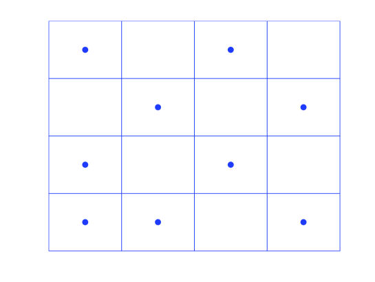
Figure 2: Minimum vortex configuration for $4\times 4$ square lattice for $f=1/2$

For $f=1/3$, the minimum vortex configuration, is shown in Fig.3. Again the checkerboard pattern is seen for the vortex configuration in the ground state. In both cases, we can see that there is an extra vortex in the boundary of the lattice. This is a boundary effect and can be ignored in large lattice limit. These results are in agreement with experimental results on rotating BEC[33, 34, 35].

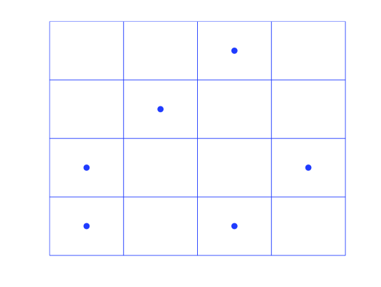
Figure 3: Minimum vortex configuration for $4\times 4$ square lattice for $f=1/3$

When number of plaquettes increases, number of possible vortex configurations, increases and we can use a combination of this method with Monte-Carlo method[36].

4 Robustness of minimum vortex configuration with respect to coupling constants

We see that in our approximation, the coupling of JJA changes as the inverted parabola. Here, we discuss the effect of changing the coupling constants on the minimum vortex configuration. We consider an inverted parabola $m_{i}$,

$$m_{ij}=16ij(i-N_{R}-1)(j-N_{C}-1)/[(N_{C}+1)^{2}(N_{R}+1)^{2}]$$ (18)

for $ij$th site of square lattice, where $N_{C}$ is the number of columns and $N_{R}$ is the number of rows. The coupling between two nearest neighbor sites on the lattice can be found from $J_{(i,j),(k,l)}=\sqrt{m_{ij}m_{kl}}$ which gives a better approximation comparing to the uniform couplings. Result for the same situation as Fig. 2, is shown in Fig. 4. It is seen that the minimum vortex configuration is not affected by the change of the coupling configuration. We have also checked the results for random $m_{ij}$ and we found the same minimum vortex configuration.

Figure 4: Minimum vortex configuration for $4\times 4$ square lattice for $f=1/2$ with non-uniform coupling.

5 Conclusion

We study a rotating BEC in a square optical lattice in a regime which Hamiltonian of the system can be mapped onto JJA. In this regime, we formulate ground state of system in terms vortex configuration. Our results in uniform coupling case, show that vortex configuration in ground state has checkerboard pattern. We have also checked the non-uniform coupling in the form $DJD$, which $D$ is a diagonal matrix, and $J$ is original uniform coupling matrix. The results for this case show that minimum vortex configuration is robust with respect to the change of coupling matrix.

References

- [1] M. H. Anderson, J. R. Ensher, M. R. Mathews, C. E. Wieman, and E. A. Cornell, Scinece 269, 198 (1995).
- [2] C. J. Pethick and H. Smith, Bose-Einstein Condensation in Dilute Gases, Cambridge University Press (2001).
- [3] J. O. Andersed, Rev. Mod. Phys. 76, 599 (2004).
- [4] O. Morsch and M. Oberthaler, Rev. Mod. Phys. 78, 179 (2006).
- [5] I. Bloch, Nature Phys. 1, 23 (2005).
- [6] M. Ben Dahan, E. Peik, J. Reichel, Y. Castin, and C. Salomon, Phys. Rev. Lett. 76, 4508 (1996).
- [7] E. Peik, M. Ben Dahan, I. Bouchoule, Y. Castin, and C. Salomon, Phys. Rev. A 55, 2989 (1997).
- [8] O. Morsch, J. H. Muller, M. Cristiani, D. Ciampini, and E. Arimondo, Phys. Rev. Lett. 87, 140402 (2001).
- [9] M. Cristiani, O. Morsch, J. H. Muller, D. Ciampini, and E. Arimondo, Phys. Rev. A 65, 063612 (2002).
- [10] S. R. Wilkinson, C. Bharucha, K. W. Madison, Q. Niu, and M. G. Raizen, Phys. Rev. Lett. 76, 4512 (1996).
- [11] F. S. Cataliotti, S. Burger, C. Fort, P. Maddaloni, F. Minardi, A. Trambettoni, A. Smerzi, and M. Inguscio, Science 293, 843 (2001).
- [12] K. Kasamatsu, J. Low Temp. Phys. 150, 593 (2008).
- [13] B. P. Anderson and M. A. Kasevich, Science 282, 1686 (1998).
- [14] K. Kasamatsu, Phys. Rev. A 79, 021604(R) (2009).
- [15] S. Levy, E. Lahoud, I. Shomroni, and J. Steinhauer, Nature 449, 579 (2007).
- [16] M. Polini, R. Fazio, M. P. Tosi, J. Sinova, and A. H. MacDonald, Laser Phys. 14, 603 (2004).
- [17] M. Polini, R. Fazio, A. H. MacDonald, and M. P. Tosi, Phys. Rev. Lett. 95, 010401 (2005).
- [18] D. Jaksch, C. Burder, J. I. Cirac, C. W. Gardiner, and P. Zoller, Phys. Rev. Lett. 81, 3108 (1998).
- [19] M. Griener, O. Mandel, T. Esslinger, T. W. Hansch, and I. Bloch, Nature (London) 415, 39 (2002).
- [20] Y. Fujihara, A. Koga, and N, Kawakami,Phys. Rev. A 79, 0131610 (2009).
- [21] T. Giamarchi, C. Ruegg, and O. Tchernyshyov, Nature Phys. 4, 198 (2008).
- [22] H. Zhai, R. O. Umucahlar, and M. O. Oktel, Phys. Rev. Lett. 104, 145301 (2010).
- [23] K. W. Madison, E. Chevy, V, Bretin, and J. Dalibard, Phys. Rev. Lett. 86, 4443 (2001).
- [24] N. R. Cooper, Advanced in Physics 57, 539 (2008).
- [25] A. L. Fetter, Rev. Mod. Phys. 81, 647 (2009).
- [26] G. Watanabe, S. A. Gafford, G. Bayam, and C. J. Pethik, Phys. Rev. A 74, 063621 (2006).
- [27] N. R. Cooper, S. Komineas, and N. Read, Phys. Rev. A 70, 033604 (2004).
- [28] A. Aftalio, X. Blanc, and J. Dalibard, Phys. Rev. A 71, 023611 (2005).
- [29] S. I. Matreenko, D. Kovrizhin, S. Ouvry, and G. V. Shlyapnikov, arXiv:0908.2172v2 [cond-mat.quant-gas] (2009).
- [30] S. Tung, V. Schweikhard, and E. A. Cornell, Phys. Rev. Lett. 97, 240402 (2006).
- [31] V. Schwiekhard, S. Tung, and E. A. Cornell, Phys. Rev. Lett. 99, 030401 (2007).
- [32] J. Zhang, C. M. Jian, F. Ye, and H. Zhai, Phys. Rev. Lett. 105, 155302 (2010).
- [33] J. W. Reijnders and R. A. Duine, Phys. Rev. Lett. 93, 060401 (2004).
- [34] J. W. Reijnders and R. A. Duine, Phys. Rev. A 71, 063607 (2005).
- [35] H. Pu, L. O. Baksmaty, S. Yi, and N. P. Biglow, Phys. Rev. Lett. 94, 190401 (2005).
- [36] Y. Azizi and A. Valizadeh, Physica B 406, 1017 (2011).
- [37] S. Teitel and C. Jayaprakash, Phys. Rev. Lett. 51, 1999 (1983).
- [38] L. Sanchez-Palencia and L. Santos, Phys. Rev. A 72, 053607 (2005).
- [39] L. Gaindini, C. Triche, P. Verkerk, and G. Grynberg, Phys. Rev. Lett. 79, 3363 (1997).
- [40] J. E. Lye, L. Fallani, M. Modugno, D. S. Wiersma, C. Fort, and M. Inguscio, Phys. Rev. Lett. 95, 070401 (2005).
- [41] A. Trombettoni, A. Smerzi, and P. Sodano, New. J. Phys. 7, 57 (2005).
- [42] F. Meier and W. Zwerger, Phys. Rev. A 64, 033610 (2001).