Finite-size scaling in two-dimensional Ising spin glass models

Abstract

We study the finite-size behavior of two-dimensional spin-glass models. We consider the $\pm J$ model for two different values of the probability of the antiferromagnetic bonds and the model with Gaussian distributed couplings. The analysis of renormalization-group invariant quantities, the overlap susceptibility, and the two-point correlation function confirms that they belong to the same universality class. We analyze in detail the standard finite-size scaling limit in terms of $TL^{1/\nu}$ in the $\pm J$ model. We find that it holds asymptotically. This result is consistent with the low-temperature crossover scenario in which the crossover temperature, which separates the universal high-temperature region from the discrete low-temperature regime, scales as $T_{c}(L)\sim L^{-{\theta_{S}}}$ with $\theta_{S}\approx 0.5$.

I Introduction

The two-dimensional (2D) Edwards-Anderson spin-glass model EA-75 has been extensively studied in recent years in order to investigate the interplay of disorder and frustration in 2D systems. If frustration is sufficiently large, these systems are paramagnetic at any finite temperature $T$. A critical glassy behavior is only observed for $T\to 0$. The zero-temperature behavior has been extensively studied. It is now well understood that it depends on the behavior of the low-energy spectrum. One should indeed distinguish systems with a discrete energy spectrum (DES), such as the $\pm J$ Ising model with a bimodal coupling distribution, from systems with a continuous energy spectrum (CES), such as the Ising model with Gaussian distributed couplings AMMP-03 ; JLMM-06 ; LMMS-06 . At $T=0$, these two classes of systems behave quite differently. For instance, in DES systems, the stiffness exponent vanishes, while in CES systems, we have $\theta<0$; recent numerical studies footnote-theta give $\theta\approx-0.28$.

For finite values of $T$, CES systems show a standard critical behavior, consistent with what is observed at $T=0$. In particular, one expects $\nu=-1/\theta$ and $\eta=0$, two predictions which are consistent with numerical data JLMM-06 ; KLC-07 . The behavior of DES systems is instead more complex. In a finite box of linear size $L$, one observes two different behaviors, which depend on how large $L$ is compared to a temperature-dependent crossover length $L_{c}(T)$; see Refs. JLMM-06 ; THM-11a ; THM-11b ; JK-11 ; PPV-10 and references therein. For $L<L_{c}(T)$, the critical behavior is analogous to that observed at $T=0$. The system shows an effective long-range spin-glass order and its critical behavior can be predicted using droplet theory THM-11a ; JK-11 . On the other hand, for $L>L_{c}(T)$, the system is effectively paramagnetic. Equivalently, at fixed $L$, one observes the two regimes for $T<T_{c}(L)$ and $T>T_{c}(L)$, respectively, where $T_{c}(L)$ is the corresponding crossover temperature. Note that this discrete behavior can only be observed for finite values of $L$, since $T_{c}(L)\to 0$ for $L\to\infty$. Of course, since $T_{c}(L)$ is an effective finite-size temperature, the crossover temperature is not uniquely defined, and many different definitions can be used. One of the basic questions is whether the critical behavior of DES systems for $T>T_{c}(L)$ is the same as that observed in CES systems. The numerical results of Ref. JLMM-06 strongly suggested that this is the case. However, those conclusions were later questioned in Ref. KLC-07 , on the basis that much larger lattices were needed to show it conclusively.

In a renormalization-group (RG) picture, the two regimes can be interpreted as due to two different fixed points (FPs) JLMM-06 ; JK-11 : a stable FP—the same that controls the critical behavior of CES systems—which describes the infinite-volume behavior up to $T=0$, and an unstable FP, present only in DES systems, which controls the low-temperature behavior for $T<T_{c}(L)$.

In order to fully specify the two regimes, one should predict how $T_{c}(L)$ scales with the size $L$. A free-energy argument, based on the energy difference and degeneracies of the two lowest-energy states KLC-07 , suggests $T_{c}(L)\sim 1/\ln L$ as $L\to\infty$. However, recently, using droplet theory, Refs. THM-11a ; THM-11b ; JK-11 suggested a power-law behavior

$$L_{c}(T)\sim T^{-1/\theta_{S}},\qquad\qquad T_{c}(L)\sim L^{-\theta_{S}}.$$ (1)

Reference THM-11a predicted $\theta_{S}\approx 0.50(1)$, which appears to be consistent with their numerical data for the twist free energy THM-11a and the two-point correlation function THM-11b , as well as with previous results SK-94 ; LMMS-06 . A calculation in a hierarchical model JK-11 gives a similar result of $\theta_{S}\approx 0.37$. These calculations indicate that although $\theta_{S}$ is quite small, it is nonetheless larger than the exponent $1/\nu=-\theta\approx 0.28$ ($\theta$ is the stiffness exponent in CES systems).

In this paper, we investigate again the question of universality, by comparing the finite-size scaling (FSS) of the $\pm J$ model for two values of the disorder parameter $p=0.5,\,0.8$ and the model with Gaussian distributed couplings (henceforth we call it the Gaussian model). The FSS analysis in terms of RG invariant quantities (for example, the plots of the Binder cumulants versus the ratio $\xi/L$, with all quantities being defined in terms of the overlap variables) shows that the two models belong to the same universality class, confirming the conclusions of Refs. JLMM-06 ; LMMS-06 . Indeed, the $\pm J$ data have the same FSS behavior as the Gaussian data, if we only consider the $\pm J$ model results corresponding to temperatures larger than the crossover temperature. Then, we focus on the validity of the standard FSS in terms of the variable $TL^{1/\nu}$, which is a rather subtle point in DES systems. Standard FSS exists only if $T_{c}(L)L^{1/\nu}\to 0$ for $L\to\infty$. If we assume $T_{c}(L)\sim L^{-\theta_{S}}$, then since $T_{c}(L)L^{1/\nu}\sim L^{1/\nu-\theta_{S}}$, FSS can be observed only if $\theta_{S}>1/\nu\approx 0.28$. This implies that if $T_{c}(L)\sim 1/\ln L$ KLC-07 ; PPV-10 , the FSS limit $T\to 0$, $L\to\infty$ at fixed $TL^{1/\nu}$ does not exist in DES systems. On the other hand, if Eq. (1) holds with $\theta_{S}\approx 0.50$, FSS holds also in DES models. However, the approach to the asymptotic limit is quite slow. The region in which no FSS is observed, which corresponds to $TL^{1/\nu}\lesssim T_{c}(L)L^{1/\nu}$, shrinks slowly, as $L^{1/\nu-\theta_{S}}\sim L^{-0.2}$. The comparison of the Monte Carlo (MC) simulations of the $\pm J$ and Gaussian models shows quite convincingly that for fixed $TL^{1/\nu}$ close to $T_{c}(L)L^{1/\nu}$, the $\pm J$ model data converge toward the data of the Gaussian model, confirming the existence of the standard FSS, hence the power-law behavior (1) with $\theta_{S}>1/\nu$. A reanalysis of the freezing temperature $T_{f}(L)$, defined in Ref. PPV-10 from the freezing of $\xi/L$ and of the Binder cumulants [at fixed $L$, they are approximately constant for $T<T_{f}(L)$], is consistent with Eq. (1) with $\theta_{S}\approx 0.4$, which is close to the estimate of Ref. THM-11a . The freezing temperature $T_{f}(L)$ should represent a correct effective definition for $T_{c}(L)$, although deviations from the universal FSS behavior are expected for somewhat larger values of $T$.

We also investigate the FSS behavior of the magnetization and the two-point correlation function of the overlap variables. We find that the data are consistent with the hyperscaling relation $2\beta=\eta\nu$. However, the data are not sufficiently precise to provide a precise determination of $\eta$, being consistent with a small value of $\eta\lesssim 0.2$, including $\eta=0$. In Ref. THM-11b , the authors showed that a properly subtracted overlap correlation function scales in the temperature region they consider, which essentially corresponds to $T\lesssim T_{c}(L)$. Here we consider the opposite regime, $T>T_{c}(L)$. We find that standard FSS as well as universality hold for the overlap correlation function.

The paper is organized as follows. In Sec. II, we define the models and the quantities we investigate. Section III reports the numerical results of our FSS analysis: in Sec. III.1, we discuss the RG invariant couplings, such as the ratio $\xi/L$ and the cumulants of the overlap variable, focusing mainly on the question of the validity of FSS in terms of $TL^{1/\nu}$; in Sec. III.2, we discuss the overlap magnetization and susceptibility; and finally, in Sec. III.3, we discuss the two-point correlation function. In Sec. IV, we present our conclusions.

II Models and definitions

We consider the 2D Ising model on a square lattice with Hamiltonian

$${\cal H}=-\sum_{\langle xy\rangle}J_{xy}\sigma_{x}\sigma_{y},$$ (2)

where $\sigma_{x}=\pm 1$, the sum is over all pairs of lattice nearest-neighbor sites, and the exchange interactions $J_{xy}$ are uncorrelated quenched random variables. We consider a model with Gaussian bond distribution,

$$P(J_{xy})\sim\exp(-J_{xy}^{2}/2)$$ (3)

(in the following, we call it the Gaussian model). We also consider the $\pm J$ model where the couplings $J_{xy}$ take values $\pm J$ with probability distribution

$$P(J_{xy})=p\delta(J_{xy}-J)+(1-p)\delta(J_{xy}+J).$$ (4)

As in Ref. PPV-10 , we consider $p=0.5$ and $0.8$. We recall that for sufficiently large frustration, i.e., for $0.11\lesssim p\lesssim 0.89$, the model shows a zero-temperature glassy critical behavior, with a paramagnetic low-temperature phase. Ferromagnetism can only be observed for $p>p^{*}=0.89093(3)$ PPV-09 .

The critical modes at the glassy transition are those related to the overlap variable $q_{x}\equiv\sigma_{x}^{(1)}\sigma_{x}^{(2)}$, where the spins $\sigma_{x}^{(i)}$ belong to two independent replicas with the same disorder realization $\{J_{xy}\}$. In our Monte Carlo (MC) simulations, we compute the overlap magnetization

$$m=\frac{1}{L^{2}}[\langle|\sum_{x}q_{x}|\rangle],$$ (5)

the overlap susceptibility $\chi$, and the second-moment correlation length $\xi$ defined from the correlation function

$$G_{o}(x)\equiv[\langle q_{0}\,q_{x}\rangle]=[\langle\sigma_{0}\,\sigma_{x}\rangle^{2}],$$ (6)

where the angular and the square brackets indicate the thermal average and the quenched average over disorder, respectively. We define $\chi\equiv\sum_{x}G_{o}(x)$ and

$$\xi^{2}\equiv\frac{1}{4\sin^{2}(p_{\rm min}/2)}\frac{\widetilde{G}_{o}(0)-\widetilde{G}_{o}(p)}{\widetilde{G}_{o}(p)},$$ (7)

where $p=(p_{\rm min},0)$, $p_{\rm min}\equiv 2\pi/L$, and $\widetilde{G}_{o}(q)$ is the Fourier transform of $G_{o}(x)$. We also consider some quantities that are invariant under RG transformations in the critical limit, which we call phenomenological couplings. We consider the ratio $\xi/L$ and the quartic cumulants

$$U_{4}\equiv\frac{[\rho_{4}]}{[\rho_{2}]^{2}},\quad U_{22}\equiv\frac{[\rho_{2}^{2}]-[\rho_{2}]^{2}}{[\rho_{2}]^{2}},$$ (8)

where $\rho_{k}\equiv\langle\;(\sum_{x}q_{x}\;)^{k}\rangle$.

In the case of a $T=0$ transition with a nondegenerate ground state, as expected in CES systems, the overlap magnetization exponent $\beta$ vanishes, and $U_{4}\to 1$ and $U_{22}\to 0$ for $T\to 0$. Moreover, assuming the hyperscaling relation $2\beta=\eta\nu$, we obtain $\eta=0$, thus $\chi\sim\xi^{2}$ for $T\to 0$.

III Finite-size scaling behavior

In order to study the FSS behavior, we extend the MC simulations of the $\pm J$ model at $p=0.5$ and $0.8$ presented in Ref. PPV-10 ; we perform further simulations of the $\pm J$ Ising model at $p=0.8$ on finite square lattices of sizes $L=16,32$, and of the Gaussian model for $L=8,12,16$. We use the Metropolis algorithm and the random-exchange method raex . For the Gaussian model, we study the temperature interval $T_{\rm min}\leq T\lesssim 1.6$, with $T_{\rm min}=0.2$ ($L=8$) and $T_{\rm min}=0.167$ ($L=12,16$). We average over a large number of disorder samples, i.e., $10^{4}$ for each $T$ and $p$.

III.1 RG invariant couplings

To begin with, we wish to check that the $\pm J$ model and the Gaussian model belong to the same glassy universality class, extending the FSS analyses of Refs. JLMM-06 ; KLC-07 ; PPV-10 . For this purpose, we consider $U_{4}$ and $U_{22}$ as a function of $\xi/L$. Our numerical results for the largest values of $L$ are reported in Fig. 1. No scaling corrections are visible in the plot of $U_{4}$, as already observed in Refs. KLC-07 ; PPV-10 , while slightly larger corrections appear in the case of $U_{22}$ for $\xi/L\gtrsim 0.6$. It is, however, evident that as $L$ increases, the differences between the Gaussian model results and those for the $\pm J$ model decrease. Thus, these results, together with those presented in Refs. JLMM-06 ; KLC-07 (in Ref. JLMM-06 , other CES and DES systems were considered), confirm that all models belong to the same universality class.

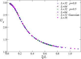
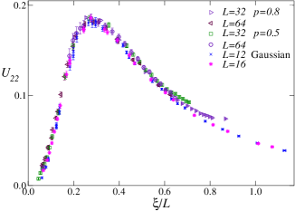
Figure 1: (Color online) The cumulants $U_{4}$ and $U_{22}$ vs $\xi/L$. We present data for the $\pm J$ model ($p=0.5$ and $0.8$) and for the Gaussian model. Only the data for the largest lattices are included for clarity.

Now we investigate the question of the existence of standard FSS as a function of $TL^{1/\nu}$. For a RG-invariant quantity $R$, we expect

$$R=h_{R}(x),\qquad\qquad x\equiv aTL^{1/\nu},$$ (9)

where $a$ is a nonuniversal constant that depends on the model but not on the quantity $R$, which can be chosen so that $h_{R}(x)$ is model independent.

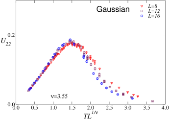
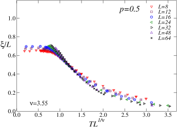
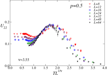
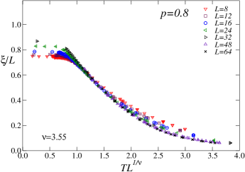
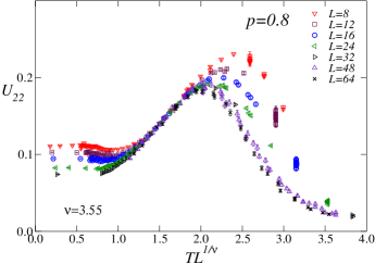
Figure 2: (Color online) The phenomenological couplings $\xi/L$ (left) and $U_{22}$ (right) vs $TL^{1/\nu}$. We report the results for the Gaussian model (top), and for the $\pm J$ model at $p=0.5$ (middle) and at $0.8$ (bottom).

First, we consider the data for the Gaussian model. The numerical results for $\xi/L$ and $U_{22}$ are reported versus $TL^{1/\nu}$ in Fig. 2 (top). We use $\nu=3.55$, which corresponds to $\theta=-1/\nu=-0.282$, which in turn is the present best estimate of the stiffness exponent of the Gaussian model footnote-theta . The data show that $\xi/L$ and $U_{22}$ scale reasonably as a function of $TL^{1/\nu}$ and clearly appear to approach a FSS limit with increasing $L$. Scaling violations increase as $TL^{1/\nu}$ increases. This is not unexpected since the correct scaling variable is the combination $u_{T}(T)L^{1/\nu}$, where $u_{T}(T)$ is the nonlinear scaling field associated with the temperature. Considering $TL^{1/\nu}$ as the scaling variable corresponds to expanding $u_{T}(T)$ to first order in the temperature, an approximation which is expected to work well only when $T$ is small. On the other hand, the region $TL^{1/\nu}\gtrsim 2$ corresponds to temperatures $T\gtrsim 1$ for the lattice sizes considered here. Of course, we cannot exclude the additional presence of nonanalytic scaling corrections, which increase as $TL^{1/\nu}$ increases.

Then, we consider the data for the $\pm J$ model; see Fig. 2. The data show essentially three types of behavior, depending on the value of $TL^{1/\nu}$. For $TL^{1/\nu}\lesssim 1.5$, no scaling is observed. This may be explained by the fact that the data in this region are below the crossover temperature, i.e., they correspond to $T<T_{c}(L)$, and thus are outside the regime in which FSS is supposed to hold. Then, there is an intermediate region, $1.5\lesssim TL^{1/\nu}\lesssim 2.0$, where data show scaling with small corrections — this is particularly evident for $U_{22}$. For $TL^{1/\nu}\gtrsim 2.0$, the corrections are larger, but the results appear to rapidly converge to a limiting curve: for both $\xi/L$ and $U_{22}$, the results satisfying $L\geq 32$ are very close to each other. We conclude that at least for $TL^{1/\nu}\gtrsim 1.5$, FSS apparently holds.

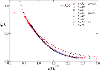
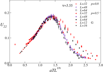
Figure 3: (Color online) The phenomenological couplings $\xi/L$ (left) and $U_{22}$ (right) versus $aTL^{1/\nu}$. We report the results for the $\pm J$ model at $p=0.8$ and $0.5$ (only $L\geq 32$) and for the Gaussian (G) model (only $L\geq 12$). We fix $a=1$, $1.5$, and $1.3$ for the Gaussian model, and for the $\pm J$ model at $p=0.8$ and $0.5$, respectively.

Furthermore, we verify the universality of the FSS behavior by comparing the results for the function $h_{R}(x)$ defined in Eq. (9). For this purpose, we should first fix the model-dependent constant $a$ that appears in Eq. (9). We determine it by requiring the FSS curves for $\xi/L$ to coincide in the region in which $\xi/L\approx 0.5$. Indeed, in this range of values of $\xi/L$, we observe small scaling deviations in all of the models we consider. If we set $a=1$ for the Gaussian model, then for the $\pm J$ model, we obtain $a(p=0.5)\approx 1.3$ and $a(p=0.8)\approx 1.5$. In Fig. 3, we plot together the data for the Gaussian model and the $\pm J$ models at $p=0.8$ and $0.5$. For clarity, we only report the data with $L\geq 32$ for the $\pm J$ model and the results with $L\geq 12$ for the Gaussian model. With this choice, there is only one point (it belongs to the $\pm J$ model with $p=0.8$ and corresponds to $L=32$) which belongs to the region $T<T_{c}(L)$. This point is clearly visible in the figures as an isolated point. If we discard it, we observe good scaling up to $aTL^{1/\nu}\lesssim 1.5$: the $\pm J$ model data and the Gaussian data fall on top of each other with good precision. For $aTL^{1/\nu}\gtrsim 1.5$, the $\pm J$ data scale reasonably. The data of the Gaussian model, which correspond to significantly smaller lattices, show significant scaling corrections. It is, however, reassuring that the trend is correct: as $L$ increases, they approach the $\pm J$ results.

In order to understand the behavior close to the crossover temperature $T_{c}(L)$, in Fig. 4 we report results for all values of $L$, but only for $aTL^{1/\nu}<1.25$. It is clear that the deviations between $\pm J$ and Gaussian data slowly decrease as $L$ increases (the same occurs for $p=0.5$, not shown). This is consistent with the idea that FSS in terms of $TL^{1/\nu}$ holds asymptotically, and, hence, with the prediction $T_{c}(L)\sim L^{-\theta_{S}}$ with $\theta_{S}>1/\nu$. The approach is, however, very slow. Indeed, the region in which FSS does not hold is predicted to shrink as $L^{-\theta_{S}+1/\nu}\sim L^{-0.2}$.

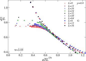
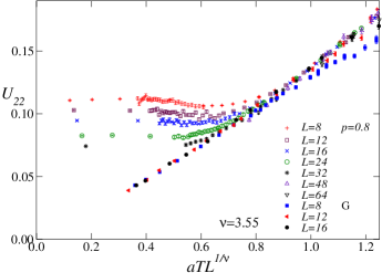
Figure 4: (Color online) The phenomenological couplings $\xi/L$ (left) and $U_{22}$ (right) vs $aTL^{1/\nu}$ for $aTL^{1/\nu}<1.25$. We report the results for the $\pm J$ model at $p=0.8$ and for the Gaussian model. We fix $a=1$ for the Gaussian (G) model and $a=1.5$ for the $\pm J$ model at $p=0.8$.

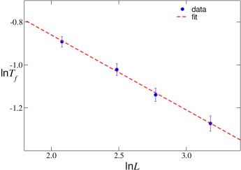
Figure 5: (Color online) Log-log plot of the freezing temperature $T_{f}(L)$ vs $L$ for the $\pm J$ model at $p=0.8$. The dashed line shows a fit to the data, corresponding to $T_{f}(L)\sim L^{-0.35}$.

This power-law behavior is also supported by the scaling of the freezing temperature $T_{f}(L)$ defined in Ref. PPV-10 . For each value of $L$, $\xi/L$ and $U_{4}$ become constant for small $T$, assuming values $(\xi/L)_{f}$ and $U_{4,f}$. Then, one defines $T_{f}(L)$ as the largest temperature of the region in which $\xi/L\approx(\xi/L)_{f}$ and $U_{4}\approx U_{4,f}$. A fit of the data to a power-law behavior logw gives $T_{f}(L)\sim L^{-0.35}$; see Fig. 5. Given the ad hoc procedure footnote-etf used to determine $T_{f}(L)$, it is difficult to give a reliable error for the result. It is, however, reassuring that the estimate satisfies the bound $\theta_{S}>1/\nu$ and is close to the estimates of Refs. LMMS-06 ; THM-11a .

III.2 Overlap magnetization and susceptibility

The overlap magnetization $m$ and susceptibility are expected to behave as

$$m=\xi^{-\beta/\nu}u_{h}(T)f_{m}(\xi/L),$$ (10)

and

$$\chi=\xi^{2-\eta}u_{h}(T)^{2}f_{\chi}(\xi/L),$$ (11)

where $f_{m}(x)$ and $f_{\chi}(x)$ are universal functions apart from a multiplicative constant, and the scaling field $u_{h}(T)$ is an analytic function of $T$. If hyperscaling holds, we should have

$$\beta=\frac{\eta\nu}{2}.$$ (12)

Thus, the combination

$$H=\frac{\xi^{2}m^{2}}{\chi}$$ (13)

should be a universal function of $\xi/L$, independent of the scaling field $u_{h}(T)$. In Fig. 6, we show the combination $H$ for the Gaussian model and the $\pm J$ model at $p=0.8$. The scaling is good. Deviations are only observed for $\xi/L\lesssim 0.2$ — these data correspond to large temperatures — and for $\xi/L\gtrsim 0.6$, which, as discussed in Ref. PPV-10 , is the region in which strong crossover effects are observed for the lattice sizes considered in this paper. However, the observed trends are consistent with a unique universal curve. We thus confirm the validity of Eq. (12), independently of what the numerical value of $\eta$ is. If, indeed, $\eta=0$, as theoretically predicted, Eq. (12) gives $\beta=0$.

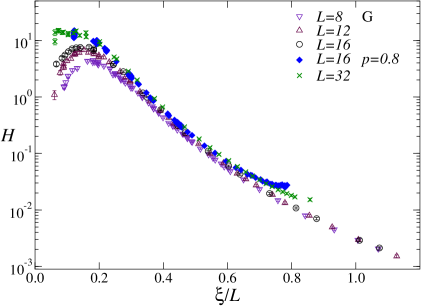
Figure 6: (Color online) Scaling combination $H$ defined in Eq. (13) vs $\xi/L$ for the Gaussian (G) model and the $\pm J$ model at $p=0.8$.

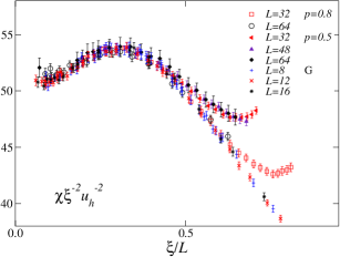
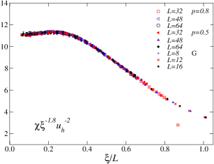
Figure 7: (Color online) Scaling combination $\chi L^{\eta-2}u_{h}^{-2}$ vs $\xi/L$. We report the results for $\eta=0$ (left) and $\eta=0.2$ (right). Data are for the Gaussian model (G) and for the $\pm J$ model with $p=0.8$ and $0.5$.

We have fitted all Gaussian data for the overlap susceptibility to Eq. (11) — more precisely to its logarithm as in Ref. PPV-10 — obtaining $\eta=0.20(7)$. The error we report is purely statistical and does not take into account possible scaling corrections. This result is slightly larger than the predicted result $\eta=0$. The discrepancy should not be taken seriously, given the small lattices we consider. A precise determination of $\eta$ in the Gaussian model requires, indeed, much larger values of $L$; see Ref. KLC-07 .

The function $f_{\chi}(x)$ is universal apart from a rescaling: if $f_{1}(x)$ and $f_{2}(x)$ are determined in two different models, we expect $f_{1}(x)=bf_{2}(x)$, where $b$ is a model-dependent constant. We now compare the estimates of the functions $f_{\chi}(x)$ for the Gaussian model and the $\pm J$ model. In Fig. 7, we report the functions (they have been rescaled so that they coincide for $\xi/L=0.3$) for the Gaussian model and the $\pm J$ model at $p=0.8$ and $0.5$. We report the curves both for $\eta=0$ and $0.2$. In Ref. PPV-10 , we observed that for $\eta=0$, the scaling was good up to $\xi/L\approx(\xi/L)_{\rm max}$, a value which had been estimated as the boundary of the crossover region before the regime in which freezing was observed. The quantity $(\xi/L)_{\rm max}$ should scale as $(\xi/L)_{c}$, i.e., the value of $\xi/L$ at the crossover temperature. Now, using Eq. (9), since $h_{\xi/L}(x)\sim x^{-\nu}$ for $x\to 0$ to recover the correct infinite-volume behavior, we have

$$(\xi/L)_{\rm max}\sim(\xi/L)_{c}\sim h_{\xi/L}[aT_{c}(L)L^{1/\nu}]\sim T_{c}(L)^{-\nu}/L\sim L^{\nu\theta_{S}-1}\sim L^{0.8},$$ (14)

where we have used $\theta_{S}=0.5$ in the last step, and the fact that $T_{c}(L)L^{1/\nu}\to 0$ for $L\to\infty$. Again note that the inequality $\theta_{S}>1/\nu$ is necessary to guarantee that $(\xi/L)_{\rm max}\to\infty$ as $L\to\infty$. By looking at the scaling behavior of $U_{22}$, Ref. PPV-10 estimated $(\xi/L)_{\rm max}\approx 0.65$ and $0.45$ for $p=0.8$ and $0.5$, respectively, in the range $32\leq L\leq 64$. For the $\pm J$ model at $p=0.5$, a similar estimate is obtained by considering the scaling behavior of the estimates of $\xi(2L)/\xi(L)$ reported in Ref. JLMM-06 . The data for the Gaussian model agree with the $\pm J$ model data for both $p=0.5$ and $0.8$ up to $(\xi/L)_{\rm max}$. Thus, the numerical results are consistent with universality and $\eta=0$.

In Ref. PPV-10 , we also observed that if we included all data in the fits, the best estimate of $\eta$ was $\eta\approx 0.2$. Indeed, in this case, the results for the overlap susceptibility showed a very good scaling up to $\xi/L\approx 0.8$. We did not take this result as an indication that $\eta=0.2$ was a more plausible estimate than $\eta=0$ because we had good reasons to discard all data beyond $\xi/L\approx(\xi/L)_{\rm max}$. Somewhat surprisingly, if we now include the data for the Gaussian model, and take $\eta=0.2$ for all models, we again observe a good universal scaling up to $\xi/L\approx 0.8$. However, the numerical results of Ref. KLC-07 exclude $\eta=0.2$ for the Gaussian model. Thus, the apparently good observed behavior cannot hold asymptotically. In view of the result $\eta=0$ of Ref. KLC-07 , as $L$ increases, the Gaussian data should become inconsistent with $\eta=0.2$.

Finally, we note that, in order to observe a good scaling behavior for the overlap susceptibility, it is crucial to include the nonlinear scaling field $u_{h}(T)$. Indeed, such a function gives a sizable contribution to our data. In the case in which we set $\eta=0$, we obtain $u_{h}(T=1)^{2}/u_{h}(T=0.2)^{2}\approx 2.2$ and $u_{h}(T=1.5)^{2}/u_{h}(T=0.2)^{2}\approx 3.3$.

III.3 Two-point function

In Ref. THM-11b , the authors analyzed the scaling behavior of the two-point function, showing that below the crossover temperature, the two-point function scales as predicted by droplet theory. Here we analyze the two-point function in the opposite regime in which we expect

$$G_{o}(r,T)={\xi^{-2}\chi}f_{G}(r/\xi,\xi/L).$$ (15)

Note that by writing the scaling behavior in this form, there is neither the need to specify $\eta$ nor to introduce the nonlinear scaling fields. Moreover, the function $f_{G}(x,y)$ is universal.

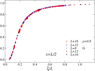
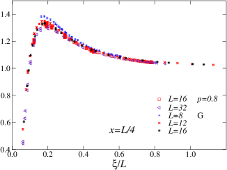
Figure 8: (Color online) Scaling combination $g_{o}(x,T)$ for $x=L/2$ (left) and $x=L/4$ (right) vs $\xi/L$. We report results for the Gaussian (G) model and the $\pm J$ model at $p=0.8$.

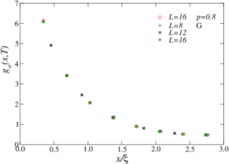
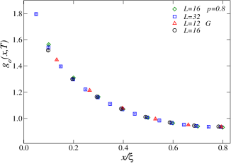
Figure 9: (Color online) Scaling combination $g_{o}(x,T)$ for $\xi/L\approx 0.18$ (left) and $\xi/L\approx 0.63$ (right) vs $x/\xi$. We report the results for the Gaussian (G) model and the $\pm J$ model at $p=0.8$.

To verify the scaling behavior (15), we compute $G_{o}(r,T)$ along a lattice line, i.e. for $r=(x,0)$. We perform the computation in the Gaussian model ($L=8,12,16$) and in the $\pm J$ model at $p=0.8$ ($L=16,32$). Then, we consider

$$g_{o}(x,T)\equiv\frac{G_{o}(r,T)L^{2}}{\chi}.$$ (16)

In Fig. 8, we report $g_{o}(x,T)$ for $x=L/2$ and $L/4$ as a function of $\xi/L$, while in Fig. 9, we show $g_{o}(x,T)$ at fixed $\xi/L\approx 0.18$ and $\xi/L\approx 0.63$ as a function of $x$. In these cases, the scaling is very good: all points fall onto a single curve, confirming the validity of Eq. (15) and universality.

IV Conclusions

We investigate the FSS behavior of two-dimensional Ising spin-glass systems. In particular, we consider the square lattice $\pm J$ model at $p=0.5$ and 0.8, and the Gaussian model. In this respect, the $\pm J$ model appears particularly problematic because it presents two different finite-volume regimes: a continuous regime for $T>T_{c}(L)$ and a discrete regime for $T<T_{c}(L)$. According to droplet theory, the crossover temperature $T_{c}(L)$ is expected to vanish in the large-$L$ limit as a power law THM-11a ; THM-11b ; JK-11 , $T_{c}(L)\sim L^{-\theta_{S}}$ with $\theta_{S}\approx 0.5$. A logarithmic behavior, $T_{c}(L)\sim 1/\ln L$, is instead suggested by the free-energy arguments of Ref. KLC-07 .

The main conclusions of our numerical analysis based on MC simulations are as follows:

• All models we consider belong to the same universality class. The magnetization, susceptibility, two-point correlation function, and the quartic cumulants, defined in terms of the overlap variables, show a universal FSS behavior in terms of $\xi/L$. In the case of the $\pm J$ model, this universal scaling is only observed above the crossover temperature $T_{c}(L)$, which separates the continuous region from the discrete low-temperature behavior.

• Our FSS analysis provides good evidence of the FSS limit $T\to 0$, $L\to\infty$ at fixed $TL^{1/\nu}$. This implies that the crossover temperature $T_{c}(L)$ does not behave as $1/\ln L$ as suggested in Ref. KLC-07 , but rather as $T_{c}(L)\sim L^{-\theta_{S}}$ with $\theta_{S}>1/\nu\approx 0.28$. This is consistent with droplet theory, which predicts a power-law behavior with $\theta_{S}\approx 0.5$.

• We study the FSS behavior of $\chi$. The data for the Gaussian and the $\pm J$ models support universality. However, the available data are not sufficient to obtain a precise estimate of $\eta$ and confirm definitely the expected value $\eta=0$.

• We verify the hyperscaling relation $2\beta=\eta\nu$. If $\beta=0$, it implies $\eta=0$.

• We consider the two-point correlation function and show that it satisfies a standard FSS ansatz. Note that the scaling form (15), which is appropriate for a high-temperature phase, is different from that considered in Ref. THM-11b , which is appropriate for a low-temperature phase in which spontaneous magnetization is present. The occurrence of these two different scaling behaviors is related to the different regimes considered. Here, we use data such that $T>T_{c}(L)$, while Ref. THM-11b studies the behavior for $T<T_{c}(L)$.

References

- (1) S. F. Edwards and P. W. Anderson, J. Phys. F: Met. Phys. 5, 965 (1975).
- (2) C. Amoruso, E. Marinari, O. C. Martin, and A. Pagnani, Phys. Rev. Lett. 91, 087201 (2003).
- (3) T. Jörg, J. Lukic, E. Marinari, and O. C. Martin, Phys. Rev. Lett. 96, 237205 (2006).
- (4) J. Lukic, E. Marinari, O. C. Martin, and S. Sabatini, J. Stat. Mech: Theory Expt., L10001 (2006).
- (5) We mention some of the most accurate estimates of the stiffness exponent at in CES models: (Ref. RSBDJR-96 ), (Ref. HY-01 ), (Ref. CBM-02 ), and (Ref. AMMP-03 ) obtained by using the Ising glass model with a Gaussian distribution for the couplings, and (Ref. LLMPV-07 ) obtained in the random-anisotropy model in the strong-anisotropy limit, whose glassy critical behavior is in the same universality class.
- (6) H. G. Katzgraber, L. W. Lee, and I. A. Campbell, Phys. Rev. B 75, 014412 (2007).
- (7) C. K. Thomas, D. A. Huse, and A. A. Middleton, arXiv:1012.3444.
- (8) C. K. Thomas, D. A. Huse, and A. A. Middleton, Phys. Rev. Lett. 107, 047203 (2011).
- (9) T. Jörg and F. Krzakala, arXiv:1104.0921.
- (10) F. Parisen Toldin, A. Pelissetto, and E. Vicari, Phys. Rev. E 82, 021106 (2010).
- (11) L. Saul and M. Kardar, Nucl. Phys. B 431, 641 (1994).
- (12) F. Parisen Toldin, A. Pelissetto, and E. Vicari, J. Stat. Phys. 135, 1039 (2009).
- (13) C. J. Geyer, in Computer Science and Statistics: Proceedings of the 23rd Symposium on the Interface, edited by E. M. Keramidas (Interface Foundation, Fairfax Station, 1991), p. 156; K. Hukushima, K. Nemoto, J. Phys. Soc. Jpn. 65, 1604 (1996); D. J. Earl, M. W. Deem, Phys. Chem. Chem. Phys. 7, 3910 (2005).
- (14) In Ref. PPV-10 , the estimates of were only compared with a logarithmic behavior, finding a reasonable consistency. Although the statistical analysis of the data favors a power-law behavior with , the available data do not really allow us to conclusively discriminate between a logarithmic and power-law approach to .
- (15) The error due to the fact that we are considering only a discrete set of temperatures varies between 0.01 and 0.04, depending on and . The estimate also slightly depends on which observable one considers.
- (16) H. Rieger, L. Santen, U. Blasum, M. Diehl, M. Jünger, and G. Rinaldi, J. Phys. A 29, 3939 (1996); 30, 8795(E) (1997).
- (17) A. K. Hartmann and A. P. Young, Phys. Rev. B 64, 180404(R) (2001)
- (18) A. C. Carter, A. J. Bray, and M. A. Moore, Phys. Rev. Lett. 88, 077201 (2002).
- (19) F. Liers, J. Lukic, E. Marinari, A. Pelissetto, and E. Vicari, Phys. Rev. B 76, 174423 (2007).