Theory of Information Pricing

Abstract

In financial markets valuable information is rarely circulated homogeneously, because of time required for information to spread. However, advances in communication technology means that the ‘lifetime’ of important information is typically short. Hence, viewed as a tradable asset, information shares the characteristics of a perishable commodity: while it can be stored and transmitted freely, its worth diminishes rapidly in time. In view of recent developments where internet search engines and other information providers are offering information to financial institutions, the problem of pricing information is becoming increasingly important. With this in mind, a new formulation of utility-indifference argument is introduced and used as a basis for pricing information. Specifically, we regard information as a quantity that converts a prior distribution into a posterior distribution. The amount of information can then be quantified by relative entropy. The key to our utility indifference argument is to equate the maximised a posterior utility, after paying certain cost for the information, with the a posterior expectation of the utility based on the a priori optimal strategy. This formulation leads to one price for a given quantity of upside information; and another price for a given quantity of downside information. The ideas are illustrated by means of simple examples.

The role and importance of information and its costing has long been recognised in economics literature Hayek . Nowadays, people often obtain information through internet search engines; but the very concept that one should search price information and utilise it to reduce expenditure, in the context of commodity markets, has been noted for at least half a century Stigler , if not considerably longer. Nevertheless, the use of information has never been as important in the past. Indeed, accesses to internet search engines—whose objectives are in information provision—constitute an integrated part of the lives of millions. Internet retailers likewise not only sell products but also provide a range of information via their recommendation engines, helping consumers find what they like but along the way also yielding additional profits. The quality of a recommendation engine, however, is difficult to assess if one cannot assign values to the information it provides.

Rapid developments in communication technology have their upsides as well as downsides. On the one hand, access to targeted information has been made easy (for example, when one knows the relevant URL from which information can be obtained), while on the other hand a generic search for specific information is becoming harder due to the flooding of irrelevant information that constitute noise. This is a phenomenon envisaged by Wiener, who used the second law of thermodynamics to explain the fact that in the long run one cannot overcome the impact of noise that overwhelms useful information, and that this effect is in part due to the advancements of communication technology wiener . Wiener also recognised that this inevitable flow can locally be reversed by means of innovations. It is for this reason that internet search engines and other information providers are constantly on alert of innovative ideas for information extraction and provision. Evidently, enhancement of information extraction and provision, and implementation of innovation, cannot be realised without cost. As a consequence, access to valuable information will likewise entail some costs. The question then is: How do we price information?

There is a form of information that is regarded as particularly valuable—the kind of information that allows one to anticipate, at least with some statistical significance, what is to come, that is, to anticipate future trends. For example, suppose that a company has just released a new product. A search engine can access various internet sites and analyse texts (e.g., blog articles and tweets) to determine how satisfied consumers are with the product. If customer satisfaction is high, the search engine can anticipate that future sales will increase and hence the company will perform well. Of course, neither the data source nor the analysis can be perfect; nevertheless, if the methodology of information extraction is adequate, then the prediction of the search engine can be statistically significant. After a while, however, sales figures are released, by which time the worth of this information diminishes.

The above example illustrates the idea of information diffusion. The search engine extracts information from in principle publicly available sources. Hence one need not be a large search engine to obtain the same information at the same time. However, in practice most people do not have the resource to analyse in real time millions of articles available on the internet. Nevertheless, after sufficient amount of time (which can be short or long), important information will be appreciated by a broad mass (and thus reflected in the share price, in the above example), diminishing the worth of information as providing predictive insights. At this stage, information has truly reached the public domain, but this is necessarily some time after its initial appearance somewhere in ‘public’.

From the viewpoint of a search or recommendation engine, and given their resources, capabilities, and objectives, therefore, it makes sense to extract useful information before the public as a whole has had chance to do so, and sell it off to a third party who is in the position to utilise this information. We can thus think of information as a tradable asset, albeit that it will have an expiry date. In order to price information, however, we must cast these intuitive ideas in terms of simple but precise mathematical language. The purpose of the present paper is to show how this is done. Our analysis reveals the surprising fact that the value of information in general need not be monotonic in the quantity of information, because sometimes less information is more useful than more information.

To illustrate how information can be valued, let us consider a simple example. Suppose that we are interested in the price tomorrow of a stock, whose current price is $s_{0}$. Our formulation of information pricing is applicable to a broader class of situations involving anticipating uncertain future events. Nevertheless, we find that the example concerning information for predicting future market very convenient for providing intuitive understanding of the theory (cf. BBMK ). To keep the discussion simple, let us assume a single-period setup so that the price $s_{0}$ today will become price $s_{1}$ tomorrow. The value of $s_{1}$ is of course unknown today, but we assume that it satisfies a known probability law $p(x)$. That is, we regard $s_{1}$ as a random variable defined on a probability space $(\Omega,{\mathcal{F}},{\mathbb{P}})$, where ${\mathbb{P}}$ denotes the physical probability measure. A search engine now performs text mining to extract information relevant to determining the value of $s_{1}$. Evidently, no search engine is capable of identifying the value of $s_{1}$; at best, it gathers noisy information in the form of signal plus noise. In the simplest setup, $s_{1}$ itself constitutes the signal, but a search engine can only extract the value of

$$\xi=s_{1}+\epsilon,$$ (1)

where $\epsilon$ represents noise, independent of $s_{1}$, with known density $f(x)$. In other words, a search engine can sample the value of $\xi$, which contains new information that is not already encoded in the value today of the stock, but not sufficient to determine the value tomorrow of the stock. With the knowledge of $\xi$ the prior density $p(x)$ of $s_{1}$ can thus be updated to the posterior density

$$\pi(x|\xi)=\frac{p(x)f(\xi-x)}{\int\mbox{$\rm d$}x\,p(x)f(\xi-x)}$$ (2)

in accordance with the Bayes formula. Writing $\pi_{\xi}(x)=\pi(x|\xi)$ for the posterior density we define the concept of information provision as follows: It is an operation that supplies the updated probability law:

$$p(x)\to\pi_{\xi}(x).$$ (3)

Stated more precisely, information provision is an updating of probability law in the form of (3) where $\pi_{\xi}(x)$ is necessarily adapted to a larger filtration (i.e. information set or knowledge) than that of $p(x)$.

Having defined the notion of information provision, we proceed to consider the pricing issues. Let us first illustrate the idea, and then try to formalise it. In the above example, an uninformed investor will use the knowledge $p(x)$ to determine the optimal asset allocation, which may contain certain amount of stock $s_{0}$, given the initial budget $W_{0}$. An informed investor is one who has purchased the knowledge $\pi_{\xi}(x)$ at a cost $c$ and used this knowledge to determine the optimal asset allocation, given a smaller initial budget $W_{0}-c$. For example, if the $p$-likelihood of stock price going up is high while the $\pi$-likelihood of this event is low, then the informed investor will purchase smaller amount of stock so as to circumvent likely loss. The problem then is to identify a fair value of the cost $c$. We would like to use a version of utility indifference argument to determine the cost. However, as we shall indicate below, for information pricing, the standard utility argument has to be augmented in a subtle manner so as to determine the fair price. Let us illustrate this by means of a simple example.

Example 1.1: uninformed investor. Consider a portfolio consisting of a single risky asset $s_{0}$ and a risk-free money market (bank) account. Let $\theta$ be the amount allocated to the money market account, and $\phi$ be the unit of stock invested. Then starting with the initial wealth $W_{0}$ we have the allocation

$$W_{0}=\theta+\phi s_{0}.$$ (4)

Let $\delta$ be the discount factor over the time period so that a unit cash invested in the money market account will yield $\delta^{-1}$ at the end of the period. Then the terminal wealth becomes

$$W_{1}=\theta\delta^{-1}+\phi s_{1}.$$ (5)

The uninformed investor will determine the optimal asset allocation strategy $(\theta^{*},\phi^{*})$ such that the expected utility ${\mathbb{E}}_{p}[U(W_{1})]$ of the terminal wealth is maximised. So for example if $s_{1}$ is a binary random variable taking values $\{0,1\}$ with probabilities $\{p,1-p\}$, and if the investor has an exponential utility

$$U(x)=1-\exp(-\alpha x)\qquad\alpha\in\mathbb{R}^{+},$$ (6)

then we have

$${\mathbb{E}}_{p}[U(W_{1})]=1-\mbox{$\rm e$}^{-\alpha\delta^{-1}(W_{0}-\phi s_{0})}\left(p+(1-p)\mbox{$\rm e$}^{-\alpha\phi}\right),$$ (7)

where we have eliminated $\theta$ by use of (4). Maximising this over $\phi$ and making use of (4), and writing ${\bar{s}}_{0}=s_{0}\delta^{-1}$ for the forwarded stock price, we obtain the following optimal asset allocation strategies:

$$\phi^{*}=\frac{1}{\alpha}\ln\left[\frac{(1-p)(1-{\bar{s}}_{0})}{p{\bar{s}}_{0}}\right],\qquad\theta^{*}=W_{0}-\phi^{*}s_{0}.$$ (8)

The optimal expected utility of terminal wealth is thus

$$u(W_{0})=1-\mbox{$\rm e$}^{-\alpha\delta^{-1}(W_{0}-\phi^{*}s_{0})}\left(p+(1-p)\mbox{$\rm e$}^{-\alpha\phi^{*}}\right).$$ (9)

Note that the optimisation has been performed without constraints. If short selling of either asset is forbidden, $(\theta^{*},\phi^{*})$ are either $(0,W_{0}/s_{0})$ or $(W_{0},0)$ depending on whether $\phi^{*}\geq W_{0}/s_{0}$ or $\phi^{*}<0$; otherwise, $(\theta^{*},\phi^{*})$ are given by (8). $\diamond$

We now consider the action of an informed investor in this simple example. We assume that there is an information provider who has the ability to sample

$$\xi=s_{1}+\epsilon,$$ (10)

where $\epsilon$ is a noise term independent of $s_{1}$, which for simplicity of exposition we assume to take values $\{0,1\}$ with probabilities $\{q,1-q\}$. In this example the value of $\xi$ can be $0$, $1$, or $2$, and the a posteriori probability $\pi_{\xi}$ that $s_{1}=0$ is given by

$$\pi_{0} = 1$$

$$\pi_{1} = \frac{p(1-q)}{p(1-q)+q(1-p)}$$ (11)

$$\pi_{2} = 0.$$

Since the information provider has to have invested capital in developing a system that is capable of sampling $\xi$, and since it has to continue investments for system maintenance, it is only reasonable to expect a payment for the provision of this information. Before we proceed to value this cost, let us first examine the strategy of an informed investor.

Example 1.2: informed investor. Let $c$ be the cost for the purchase of information. Then the initial budget condition for the informed investor becomes

$$W_{0}=\vartheta+\varphi s_{0}+c,$$ (12)

where $(\vartheta,\varphi)$ denote portfolio positions of the informed investor. An application of the optimisation procedure described above then yields:

$$\varphi^{*}=\frac{1}{\alpha}\ln\left[\frac{(1-\pi_{\xi})(1-{\bar{s}}_{0})}{\pi_{\xi}{\bar{s}}_{0}}\right],\qquad\vartheta^{*}=W_{0}-c-\varphi^{*}s_{0},$$ (13)

where $\pi_{\xi}={\mathbb{P}}(s_{1}=0|\xi)$. In this case, utility of the optimal terminal wealth is given by

$$u_{c}(W_{0})=1-\mbox{$\rm e$}^{-\alpha\delta^{-1}(W_{0}-c-\varphi^{*}s_{0})}\left(\pi_{\xi}+(1-\pi_{\xi})\mbox{$\rm e$}^{-\alpha\varphi^{*}}\right).$$ (14)

Similarly to the previous example, these results are based on unconstrained optimisation. If short selling is not permitted, for instance, then these results hold if $0\leq\varphi^{*}\leq(W_{0}-c)/s_{0}$; otherwise we must take appropriate boundary values. $\diamond$

We are now in the position to discuss valuation of information in the above examples. To this end we would like to employ an argument based on utility indifference, similar to the one presented, for example, by Grossman and Stiglitz GrossmanStiglitz . The argument intuitively goes as follows. If possession of extra information at no cost provides on average a better payoff, then every investor would sought to be informed. Consequently, there should be a positive value assigned to this information. If on the other hand the price is too high, then no one would want to be informed. Hence there exists an equilibrium level for the cost of information at which investors are indifferent, as far as their preferences are concerned.

Naively, one might then identify the utility indifferent price of information by solving the following equation for $c$:

$$u(W_{0})=u_{c}(W_{0})$$ (15)

so that the expected utility of the a posteriori optimal strategy after paying for the information equals the utility of the a priori optimal strategy. This is in effect the pricing formula proposed by Amendinger et al. Schweizer (see also Imkeller ). The intuition behind this relation is as follows: Provided that the cost $c$ is sufficiently small, the possession of additional relevant knowledge, in the form of a strictly larger filtration, necessarily increases expected utility. Since utility is a decreasing function of the cost $c$, there must be a positive number $c^{*}$ such that (15) is satisfied for $c=c^{*}$. In the context of information pricing, however, this intuitive argument fails to determine the correct value of $c^{*}$. With a further reflection, the reason for this becomes apparent: Ignorance can make people happy. While it is true that with the additional knowledge an investor will on average perform better (cf. BDFH ), an uninformed investor can be more optimistic about the future outlook. Take, for instance, an extreme case where the a priori probability that the stock price moving up by a significant amount is high. An uninformed investor will thus put the majority of the initial wealth into purchasing this stock. Suppose, however, that the a posteriori probability indicates that the stock price is more likely to move down. An informed investor will thus only invest a small fraction of the initial wealth into this stock to avoid a large loss. In this case, a likely scenario is that an informed investor knows that there is little prospect of making a large profit (i.e. small utility), but manages to prevent a loss, while an uninformed investor has a very high hope (i.e. large utility), but ending up with a loss. According to the pricing formula (15), therefore, the information cost becomes negative in such a scenario.

Grossman and Stiglitz GrossmanStiglitz (see also ver ; kyle ; peress ), on the other hand, propose the use of the following identity to fix the cost:

$${\mathbb{E}}_{p}[U(W_{p}^{*})]={\mathbb{E}}_{p}[U(W_{\pi,c}^{*})].$$ (16)

Here, $W_{p}^{*}=\theta^{*}\delta^{-1}+\phi^{*}s_{1}$ denotes the random variable associated with the terminal wealth based on the implementation of the a priori optimal strategy (8); whereas $W_{\pi,c}^{*}=\vartheta^{*}\delta^{-1}+\varphi^{*}s_{1}$ denotes the random variable associated with the terminal wealth based on the implementation of the a posteriori optimal strategy (13), having paid $c$ for the information. In the present example, (16) leads to the pricing formula

$$c^{*}=\frac{\delta}{\alpha}\ln\left[\frac{1}{q^{{\bar{s}}_{0}}(1-q)^{1-{\bar{s}}_{0}}}\right].$$ (17)

The shortcoming of the Grossman-Stiglitz pricing formula (16), however, is that the cost is fixed irrespective of its quality. For example, if the realised value of $\xi$ is either $0$ or $2$, and if there is no cap on short selling, then an investor can purchase this information for a modest cost to make infinite profit, leading to an arbitrage because starting with zero initial wealth $W_{0}=0$ one can construct a portfolio such that ${\mathbb{E}}[W_{1}]=\infty$ under any measure equivalent to ${\mathbb{P}}$. In contrast, in our theory we would like the cost of information be infinite, if this information were to provide infinite benefit.

With this in mind, we deduce that the ‘correct’ pricing formula is given by solving

$${\mathbb{E}}_{\pi}[U(W_{p}^{*})]={\mathbb{E}}_{\pi}[U(W_{\pi,c}^{*})]$$ (18)

for $c$. In other words, we consider with hindsight what would have happened to the uninformed strategy, and compared this with the informed strategy. In this way, a consistent price for information can be deduced. We propose this to be the basis with which information can be priced using a utility indifference argument.

Figure 1: Left: Expected utilities ${\mathbb{E}}_{\pi}[U(W_{p}^{*})]$ for $\xi=0,1,2$ as a function of the cost $c$ are shown here as three horizontal lines. For each value of $\xi$ we also plot ${\mathbb{E}}_{\pi}[U(W_{\pi,c}^{*})]$, when short selling is strictly prohibited. When $c$ is sufficiently small, the latter utilities are higher, but as the cost increases, they decrease. At $c=c^{*}$ the two utility functions for each $\xi$ agree and determine the unique equilibrium price for which the investor is indifferent. Here we have chosen parameters to be $\alpha=0.1$, $s_{0}=0.5$, $W_{0}=5$, $p=0.4$, $q=0.7$, and $\delta=0.95$. The numerical values for the cost for each $\xi$ are plotted as a histogram on the right side. In this example, we have $c^{*}(0)=1.51$, $c^{*}(1)=0.71$, and $c^{*}(2)=1.65$. The average cost is ${\bar{c}}^{*}=1.10$.

In the case of the above example, (18) amounts to solving

$$\mbox{$\rm e$}^{-\alpha\delta^{-1}(W_{0}-\phi^{*}s_{0})}\left(\pi_{\xi}+(1-\pi_{\xi})\mbox{$\rm e$}^{-\alpha\phi^{*}}\right)=\mbox{$\rm e$}^{-\alpha\delta^{-1}(W_{0}-c-\varphi^{*}s_{0})}\left(\pi_{\xi}+(1-\pi_{\xi})\mbox{$\rm e$}^{-\alpha\varphi^{*}}\right)$$ (19)

for $c$. This gives

$$c^{*}=\frac{\delta}{\alpha}\ln\left[\frac{\pi_{\xi}\mbox{$\rm e$}^{\alpha{\bar{s}}_{0}\phi^{*}}+(1-\pi_{\xi})\mbox{$\rm e$}^{\alpha\phi^{*}({\bar{s}}_{0}-1)}}{\pi_{\xi}\mbox{$\rm e$}^{\alpha{\bar{s}}_{0}\varphi^{*}}+(1-\pi_{\xi})\mbox{$\rm e$}^{\alpha\varphi^{*}({\bar{s}}_{0}-1)}}\right],$$ (20)

which makes it apparent that when $\phi^{*}=\varphi^{*}$, i.e. when $\xi$ provides no additional information (which can happen in the present example if for instance $p=q=\frac{1}{2}$ and $\xi=1$), or when the additional information provided by $\xi$ results in no change of the strategy, the cost is identically zero. Note that the dependence of $\pi_{\xi}$ on $\xi$ implies that the value of $c^{*}$ also depends on $\xi$. Thus, for instance if $\xi=0$ or $\xi=2$, and if unlimited short selling is allowed, then $c^{*}=\infty$ as desired. In many cases the dependence on $\xi$ is natural, because different values of $\xi$ embody different information contents. On the other hand, there are likewise many cases where it is desirable to associate fixed price for information. This applies to the provision of generic information, whereas for the purchase of a specialised information, it might be unreasonable to expect a flat rate for the information, irrespective of its content or quality. We shall therefore consider both cases.

If short selling is prohibited, then even with the knowledge $\xi=0$ or $\xi=2$ an investor can only make finite profit. Hence in this case the cost should also be strictly bounded. In figure 1 on the left panel we plot ${\mathbb{E}}_{\pi}[U(W_{p}^{*})]$ for three values of $\xi$ as functions of $c$ (clearly, ${\mathbb{E}}_{\pi}[U(W_{p}^{*})]$ for each value of $\xi$ is constant in $c$), and compared these with ${\mathbb{E}}_{\pi}[U(W_{\pi,c}^{*})]$ as functions of $c$, when short selling is forbidden. For each value of $\xi$ the intersection of the two functions determine the cost $c^{*}(\xi)$, shown as a histogram also in figure 1. For the parameter values chosen in this example, the ‘upside’ information (when $\xi=2$) is worth a little more than the ‘downside’ information (when $\xi=0$). In this way we are able to assign prices for information of specific quality. If we are interested in assigning a flat rate ${\bar{c}}^{*}$, then we average individual cost according to

$${\bar{c}}^{*}=\sum_{k}{\mathbb{P}}(\xi=\xi_{k})c^{*}(\xi_{k}).$$ (21)

In the present example we have ${\mathbb{P}}(\xi=0)=pq$, ${\mathbb{P}}(\xi=1)=p(1-q)+(1-p)q$, and ${\mathbb{P}}(\xi=2)=(1-p)(1-q)$, which can be used to determine ${\bar{c}}^{*}$. Since the a priori expectation of our pricing formula (18) gives the Grossman-Stiglitz formula (16), we see that solutions to (16) and (18) correspond, respectively, to an annealed average and a quenched average often considered in the spin-glass theory. In particular, on account of Jensen’s inequality we see that the Grossman-Stiglitz cost is the lower bound of our flat-rate cost ${\bar{c}}^{*}$.

Having introduced our framework for information pricing, the next objective in this paper is to express the cost in terms of the quantity of information so that we are able to quote the price in the form, for example: “$\pounds$X for Y bits of upside information”. This is highly desirable because the representation of the cost as a function of $\xi$ is not very practical. Our definition of information as a quantity that generates the transformation (3) allows us to proceed by the consideration of relative entropy between the a priori and the a posteriori probabilities. The examples considered above, however, are too restrictive, because the a priori and the a posteriori probabilities are not absolutely continuous with respect to each other, and thus relative entropy cannot be defined. Indeed, the idea that an information provider can ascertain the future value $s_{1}$ at time $0$, which would be the case if the sampled value of $\xi$ is either $0$ or $2$, is somewhat artificial and unrealistic. We therefore consider another simple example in which this issue does not arise.

Example 2.1: uninformed investor. We assume the setup as in Example 1.1 above, except that the random variable $s_{1}$ is assumed normally distributed with mean $\mu$ and variance $\sigma^{2}$. Thus, the model is similar to the Bachelier model, rather than a geometric Gaussian model, in that the asset price can take negative values. A straightforward Gaussian integration then gives the expected utility of terminal wealth as:

$${\mathbb{E}}_{p}[U(W_{1})]=1-\exp\left[-\alpha\left(\delta^{-1}(W_{0}-\phi s_{0})+\phi\mu-\mbox{$\textstyle\frac{1}{2}$}\alpha\phi^{2}\sigma^{2}\right)\right].$$ (22)

It follows that the optimal allocation strategy is determined by

$$\phi^{*}=\frac{\mu-{\bar{s}}_{0}}{\alpha\sigma^{2}},\qquad\theta^{*}=W_{0}-\frac{(\mu-{\bar{s}}_{0})s_{0}}{\alpha\sigma^{2}}.$$ (23)

If there is a restriction on short selling, then these results hold provided that $0\leq\phi^{*}\leq W_{0}/s_{0}$; otherwise, $\phi^{*}=0$ or $\phi^{*}=W_{0}/s_{0}$. $\diamond$

Example 2.2: informed investor. An informed investor is able to purchase the sampled value of $\xi$ given by (1) above, except that the noise variable $\epsilon$ is now assumed normally distributed with mean zero and variance $\sigma_{\epsilon}^{2}$. In this case, a standard result in Gaussian filtering theory wiener2 shows that the a posteriori probability law for $s_{1}$ given $\xi$ is also normally distributed:

$$s_{1}|_{\xi}\sim N\left(\frac{\mu\sigma^{2}_{\epsilon}+\xi\sigma^{2}}{\sigma^{2}_{\epsilon}+\sigma^{2}},\sqrt{\frac{\sigma^{2}\sigma^{2}_{\epsilon}}{\sigma^{2}+\sigma^{2}_{\epsilon}}}\right)\equiv N(\mu_{\xi},\sigma_{\xi})$$ (24)

The optimisation problem thus reduces to maximising

$$u_{c}(W_{0})=1-\exp\left(-\alpha\left(\delta^{-1}(W_{0}-c-\varphi s_{0})+\varphi\mu_{\xi}-\mbox{$\textstyle\frac{1}{2}$}\alpha\varphi^{2}\sigma^{2}_{\xi}\right)\right).$$ (25)

The result is

$$\varphi^{*}=\frac{\mu_{\xi}-{\bar{s}}_{0}}{\alpha\sigma^{2}_{\xi}},\qquad\vartheta^{*}=W_{0}-c-\frac{(\mu_{\xi}-{\bar{s}}_{0})s_{0}}{\alpha\sigma^{2}_{\xi}}.$$ (26)

As before, if short selling is not permitted, we have the conditions $0\leq\varphi^{*}\leq(W_{0}-c)/s_{0}$ for which (26) is valid; otherwise we must take boundary values. $\diamond$

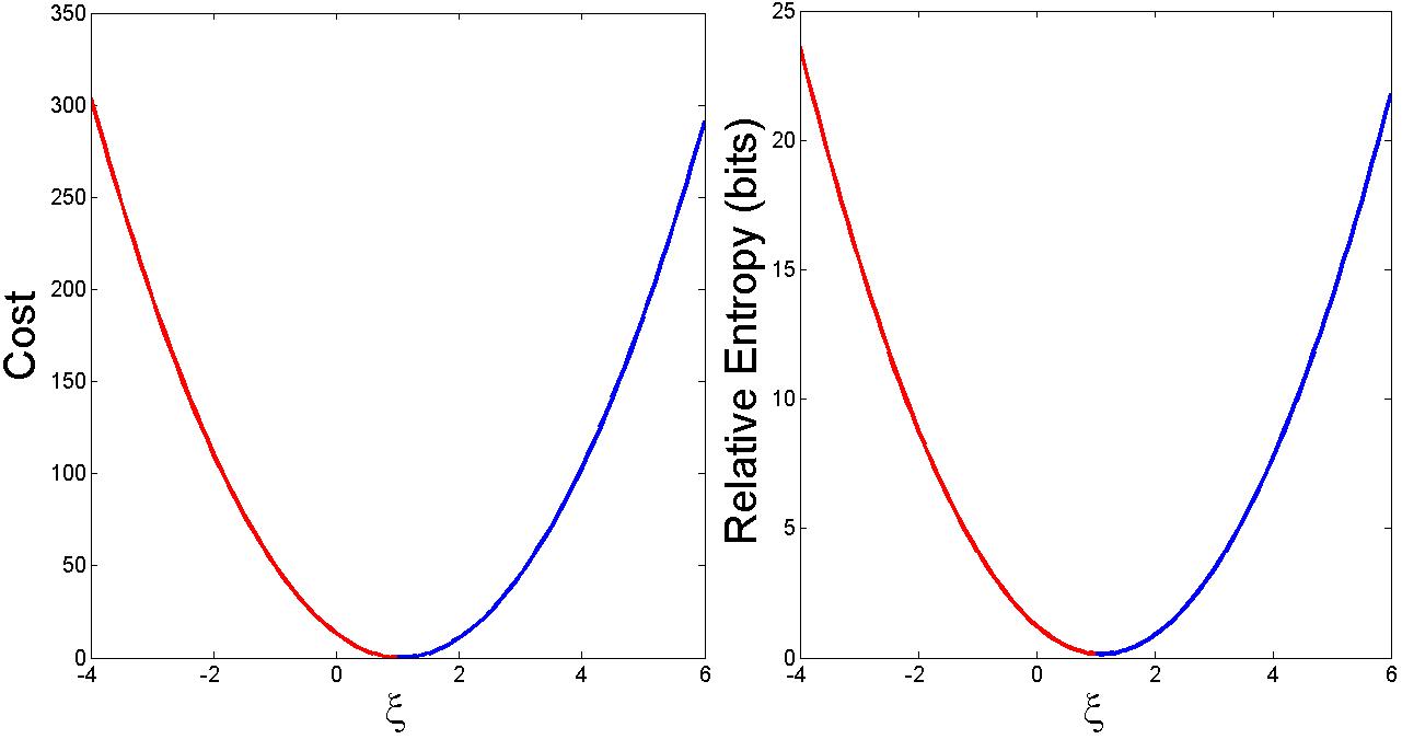
Figure 2: Left: Cost $c^{*}(\xi)$ as a function of the realised value of $\xi$. Right: Relative entropy $I(\xi)=I(\pi_{\xi}|p)$ as a function of the realised value of $\xi$. The parameter values used here are: $s_{0}=1$, $\delta=0.95$, $\alpha=0.1$, $W_{0}=10$, $\mu=1.1$, $\sigma^{2}=0.2$, $\mu_{\epsilon}=0$, and $\sigma^{2}_{\epsilon}=0.2$. The red curves correspond to pieces of downside information (i.e. values of $\xi$ that indicate decrease in $s_{1}$ as compared to the a priori expectation) and the blue curves correspond to upside information.

Let us evaluate the cost of information by the principle (18). This amounts to finding the value for $c$ that solves

$$\exp\left[-\alpha\left((W_{0}-\phi^{*}s_{0})\delta^{-1}+\phi^{*}\mu_{\xi}-\mbox{$\textstyle\frac{1}{2}$}\alpha\phi^{*2}\sigma_{\xi}^{2}\right)\right]$$

$$\qquad=\exp\left[-\alpha\left((W_{0}-c-\varphi^{*}s_{0})\delta^{-1}+\varphi^{*}\mu_{\xi}-\mbox{$\textstyle\frac{1}{2}$}\alpha\varphi^{*2}\sigma^{2}_{\xi}\right)\right],$$ (27)

with the solution

$$c^{*}=\mbox{$\textstyle\frac{1}{2}$}\alpha\delta\sigma_{\xi}^{2}(\phi^{*}-\varphi^{*})^{2}.$$ (28)

This provides the cost $c^{*}(\xi)$ as a function of the sampled value of $\xi$. That is, before the purchase is made, a client of the information provider can agree to the price structure (28) so that depending on which value of $\xi$ the information provider produces, the client will pay the cost appropriate for that information. If the use of a flat rate ${\bar{c}}^{*}$ for the cost is desirable, then we average $c^{*}(\xi)$ over $\xi$ under the suitable Gaussian measure. This is given by

$${\bar{c}}^{*}=\frac{1}{2\alpha}\delta\sigma^{2}_{\xi}\left[(\mu-\bar{s}_{0})^{2}\left(\sigma^{-2}-\sigma_{\xi}^{-2}\right)^{2}+\frac{\sigma^{2}}{\sigma^{2}_{\xi}\sigma^{2}_{\epsilon}}\right].$$ (29)

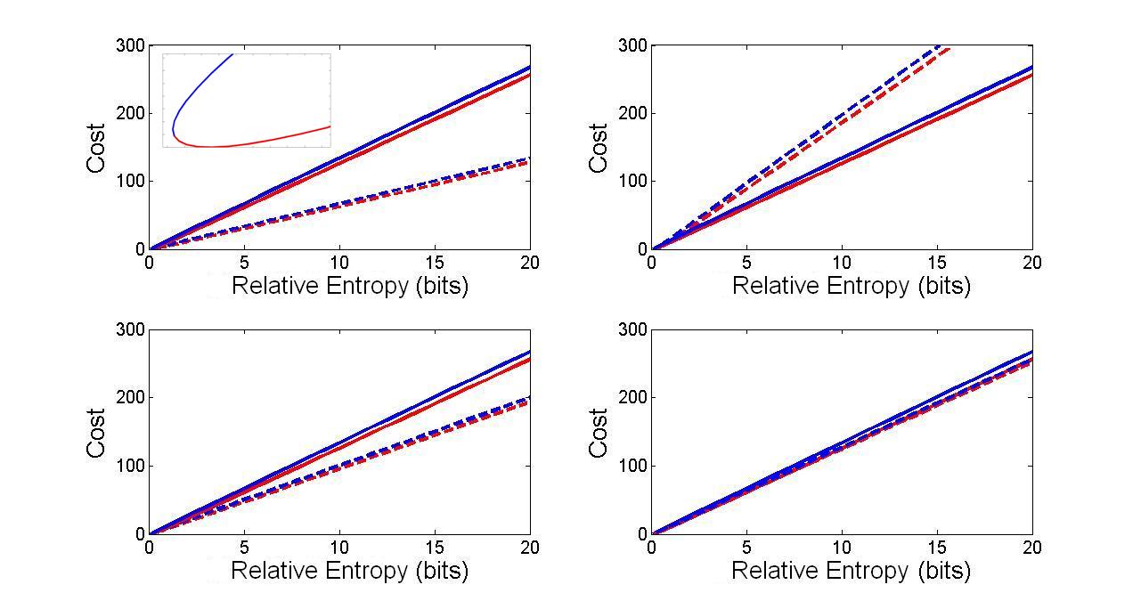
Figure 3: The cost $c^{*}(I)$ as a function of the quantity of information $I$, when there is no constraint for short selling. The solid lines in all four plots (they are identical) correspond to the parameter values used in figure 2. While keeping other parameters fixed, the following changes in parameter values are used, represented by dashed lines in the plots. Top left: $\alpha$ has been increased to $\alpha=0.2$; top right: $\sigma^{2}$ has been increased to $\sigma^{2}=0.4$; bottom left: $\sigma^{2}_{\epsilon}$ has been increased to $\sigma^{2}_{\epsilon}=0.4$; and bottom right: $\delta$ has been decreased to $\delta=0.92$. The red curves correspond to downside information, and the blue curves correspond to upside information. The insert shows the behaviour of $c^{*}(I)$ close to the origin where $c^{*}(I)$ is decreasing in $I$.

As indicated above, we wish to associate cost with the quantity of information. For this purpose, we consider the relative entropy:

$$I(\pi_{\xi}|p) = \int_{-\infty}^{\infty}\pi_{\xi}(s)\ln\left(\frac{\pi_{\xi}(s)}{p(s)}\right)\mbox{$\rm d$}s$$ (30)

$$= \mbox{$\textstyle\frac{1}{2}$}\left[\ln\left(\frac{\sigma^{2}}{\sigma^{2}_{\xi}}\right)+\frac{\sigma^{2}_{\xi}}{\sigma^{2}}-1\right]+\mbox{$\textstyle\frac{1}{2}$}\frac{(\mu_{\xi}-\mu)^{2}}{\sigma^{2}}$$

between the prior and the posterior densities. It should be evident from the decomposition $\xi=s_{1}+\epsilon$ that there is a critical value $\xi^{\dagger}$, given by the a prior expectation of $s_{1}$, such that the a posteriori density is least informative, and such that the information content increases as the value of $\xi$ increases or decreases away from this critical level. In other words, relative entropy is monotonically decreasing in $\xi$ if $\xi<\xi^{\dagger}$, and monotonically increasing in $\xi$ if $\xi\geq\xi^{\dagger}$. One might therefore expect that the cost should also exhibit the same monotonic dependence on $|\xi-\xi^{\dagger}|$. Surprisingly, however, this is not the case. The pricing formula (28) in the Gaussian model shows that if the additional information does not alter portfolio positions, then an investor is not going to pay for that information. As a consequence, minimum information can be more costly (i.e. useful) than a larger quantity of information.

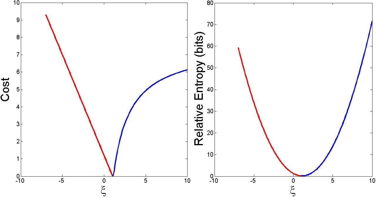
Figure 4: Left: Cost $c^{*}(\xi)$ as a function of the realised value of $\xi$ when short selling is strictly prohibited. Right: Relative entropy $I(\xi)=I(\pi_{\xi}|p)$ as a function of the realised value of $\xi$. The cost $c^{*}(\xi)$ measures the usefulness of information, while relative entropy $I(\xi)$ measures the quantity of information. The parameter values used here are: $s_{0}=1$, $\delta=0.95$, $\alpha=0.1$, $W_{0}=10$, $\mu=1.1$, $\sigma^{2}=0.2$, $\mu_{\epsilon}=0$, and $\sigma^{2}_{\epsilon}=0.2$. The red curves correspond to pieces of downside information (i.e. values of $\xi$ that indicate decrease in $s_{1}$ as compared to the a priori expectation) and the blue curves correspond to upside information.

In figure 2 we plot the cost function $c^{*}(\xi)$ where there are no constraints for short selling, and the relative entropy $I(\xi)$. By inverting these two functions we can determine the cost $c^{*}(I)$ as a function of the information content, as shown in figure 3 for a range of parameter values. Note that in the numerical plots we have converted the logarithmic basis so that relative entropy $I$ is measured in the conventional binary units of ‘bits’ rather than the Shannon units used in (30). Hence the horizontal axis represents information content expressed in binary units. We observe that costs of upside information in these examples are always slightly higher than those of downside information, and that in each case the cost is approximately a linear function of the quantity of information. We also find that the cost in the unconstrained case is a decreasing function of the risk aversion parameter $\alpha$ in the utility function, an increasing function of the signal uncertainty $\sigma$, a decreasing function of the noise uncertainty $\sigma_{\epsilon}$, and a slightly increasing function of the discount factor $\delta$.

The cost structure changes somewhat if we restrict short selling. This is because the upside gain from exploiting additional information is restricted in this case. In particular, if short selling (including cash borrowing) is prohibited, then the cost is bounded above by the initial wealth $W_{0}$. We plot in figure 4 the cost $c^{*}(\xi)$ as a function of $\xi$ in the case for which short selling is strictly forbidden. The result reveals some interesting insights: a client of an information provider is willing to pay significantly higher costs for large downside information, as compared to upside information, and the increase in $c^{*}(\xi)$ for upside information is satiated relatively early. This feature of course is closely related to the model setup chosen here: Since $s_{1}$ is assumed Gaussian, purchase of the stock by any amount can result in an unbounded loss. Therefore, investors are willing to spend the totality $W_{0}$ of the initial budget as a protection against large losses, leaving behind no asset for any investment. Conversely, investors are inclined not to spend significant portions of the initial budget on upside information, because if there are opportunities to profit from investments, they would not want to lose these opportunities by spending all the budgets.

Figure 5: The cost $c^{*}(I)$ as a function of the quantity of information $I$, when short selling is strictly prohibited. The solid lines in all four plots (they are identical) correspond to the parameter values used in figure 4. While keeping other parameters fixed, the following changes in parameter values are used, represented by dashed lines in the plots. Top left: $\alpha$ has been increased to $\alpha=0.2$; top right: $\sigma^{2}$ has been increased to $\sigma^{2}=0.4$; bottom left: $\sigma^{2}_{\epsilon}$ has been increased to $\sigma^{2}_{\epsilon}=0.4$; and bottom right: $\delta$ has been decreased to $\delta=0.92$. The red curves correspond to downside information, and the blue curves correspond to upside information.

Although the cost structure changes when there are constraints, we can again invert these relations to quote unique prices for upside and downside information. The results are shown in figure 5 for a range of parameter values. We observe that when there are constraints the price of information exhibits somewhat nontrivial behaviours as we change the model parameters.

The two cases examined here can be interpolated by gradually relaxing the borrowing cap, as shown in figure 6. These intermediate cases are often more realistic because of leveraging. In the case of the example considered here we observe that by raising the cap of borrowing to five times the total wealth the net effect is already equivalent to allowing for unlimited borrowing. The effect of leveraging is also of interest in showing in which way the upside and downside information costs intertwine.

We conclude by remarking that the existence of information asymmetries is not only fundamental to modern microeconomic theory NobelIntro but also constitutes the basis for the existence of information providers, whose roles are becoming increasingly more important in modern society. Our main objective here is to demonstrate in which way valuable information can be priced in a rational manner. Although the models used here to illustrate our pricing theory are simple, they nevertheless provide a useful conceptual guideline for evaluating information in a variety of contexts. It would be of interest to extend the single-period models considered here to continuous-time models within the context of utility indifference pricing theory (as outlined, e.g., in Schweizer ; Imkeller ; Monoyios08 ).

The authors thank Bernhard Meister for comments. DCB acknowledges Fraunhofer ITWM, Kaiserslautern, for hospitality while part of this work was carried out.

Figure 6: Interpolation of the information price $c^{*}(I)$ from the strictly constrained case to the unconstrained case. Top row, from left: (i) borrowing is strictly forbidden; (ii) borrowing is capped at $W_{0}/2$; (iii) borrowing is capped at $W_{0}$. Bottom row, from left: (i) borrowing is capped at $2W_{0}$; (ii) borrowing is capped at $5W_{0}$; (iii) unlimited borrowing permitted.

References

- (1) Hayek, F. A. The use of knowledge in society. The American Economics Review, XXXV 519–530, 1945.
- (2) Stigler, G. J. The economics of information. The Journal of Political Economy, LXIX, 213–225, 1961.
- (3) Wiener, N. The Human Use of Human Beings. (Boston: Houghton Mifflin Co., 1954).
- (4) Brody, D. C., Brody, J., Meister, B. K. & Parry, M. F. 2010 Informational inefficiency in financial markets. (arXiv:1003.0764).
- (5) Grossman, S. J. and Stiglitz, J. E. On the impossibility of informationally efficient markets. The American Economic Review, 70, 393–408, 1980.
- (6) Amendinger, J., Becherer, D. and Schweizer, M. A monetary value for initial information in portfolio optimization. Finance Stochastics, 7, 29–46, 2003.
- (7) Ankirchner, S., Dereich, S. and Imkeller, P. The Shannon information of filtrations and the additional logarithmic utility of insiders. The Annals of Probability, 34, 743–778, 2006.
- (8) Brody, D. C., Davis, M. H. A., Friedman, R. L. and Hughston, L. P. Informed traders. Proceedings of the Royal Society London A465, 1103-1122, 2009.
- (9) Verrecchia, R. E. Information acquisition in a noisy rational expectations economy. Econometrica, 50, 1415–1430, 1982.
- (10) Kyle, A. S. Informed speculation with imperfect competition. The Review of Economic Studies,, 56, 317–355, 1989.
- (11) Peress, J. Information vs. entry costs: What explains U.S. stock market evolution? The Journal of Financial and Quantitative Analysis, 40, 563–594, 2005.
- (12) Wiener, N. Cybernetics or Control and Communication in the Animal and the Machine. (Cambridge, Mass.: The Technology Press, 1948).
- (13) Löfgren, K. G., Persson, T. and Weibull, J. W. Markets with asymmetric information: The contributions of George Akerlof, Michael Spence and Joseph Stiglitz. The Scandinavian Journal of Economics, 104, 195–211, 2002.
- (14) Monoyios, M. Utility indifference pricing with market incompleteness. In Nonlinear Models in Mathematical Finance: New Research Trends in Option Pricing, pp. 67-100. M. Ehrhardt, ed. (Hauppage, New York: Nova Science Publishers, 2008).