Non-Gaussian errors of baryonic acoustic oscillations

Abstract

We revisit the uncertainty in baryon acoustic oscillation (BAO) forecasts and data analyses. In particular, we study how much the uncertainties on both the measured mean dilation scale and the associated error bar are affected by the non-Gaussianity of the non-linear density field. We examine two possible impacts of non-Gaussian analysis: (1) we derive the distance estimators from Gaussian theory, but use 1000 N-Body simulations to measure the actual errors, and compare this to the Gaussian prediction, and (2) we compute new optimal estimators, which requires the inverse of the non-Gaussian covariance matrix of the matter power spectrum. Obtaining an accurate and precise inversion is challenging, and we opted for a noise reduction technique applied on the covariance matrices. By measuring the bootstrap error on the inverted matrix, this work quantifies for the first time the significance of the non-Gaussian error corrections on the BAO dilation scale. We find that the variance (error squared) on distance measurements can deviate by up to 12% between both estimators, an effect that requires a large number of simulations to be resolved. We next apply a reconstruction algorithm to recover some of the BAO signal that had been smeared by non-linear evolution, and we rerun the analysis. We find that after reconstruction, the rms error on the distance measurement improves by a factor of $\sim 1.7$ at low redshift (consistent with previous results), and the variance ($\sigma^{2}$) shows a change of up to 18% between optimal and sub-optimal cases (note, however, that these discrepancies may depend in detail on the procedure used to isolate the BAO signal). We finally discuss the impact of this work on current data analyses.

1 Introduction

Ever since acoustic peaks were detected in the cosmic microwave background (Miller et al, 1999) and galaxy surveys (Eisenstein et al, 2005), much effort has been devoted to use baryon acoustic oscillations (BAO) as standard rulers to estimate cosmological distances with precision (Eisenstein, 2005; Blake & Glazebrook, 2003; Seo & Eisenstein, 2003; Bassett & Hlozek, 2009; McDonald & Eisenstein, 2007). BAO signals are manifested as a wiggly feature in the matter power spectrum, and precise measurements could shed light on the dynamics of dark energy. The accuracy and precision of such measurement depends directly on the covariance matrix of the matter power spectrum, which is straightforward to compute for a Gaussian density field using Wick’s theorem. However, it is known that non-Gaussianities are significant in that covariance matrix (Meiksin & White, 1999; Scoccimarro et al, 1999; Rimes & Hamilton, 2005, 2006; Takahashi et al, 2011) and may have an impact on cosmological distance measurements. A non-linear model is needed for a non-Gaussian calculation, hence some criterion for the accuracy of such effects is needed to quantify the precision of the measurement. In particular, an optimal BAO measurement should in general incorporate a proper error weighting of the data, which involves the inversion of the full covariance matrix. The accuracy criterion must therefore be based on the confidence we have on the inverted matrix.

The estimator constructed in most forecasts and data analyses follow the prescription of Seo & Eisenstein (2007), which is a procedure that constructs both the estimator of the BAO scale and the estimator of its uncertainty under the Gaussian assumption. The method was originally cross-checked with a $\chi^{2}$ analysis of $51$ simulations, including a jackknife sub-sampling of the N-body data, and showed good agreement. The actual deviation between this proposed estimator and the optimal estimator constructed in this paper is indeed small, therefore consistent with the work of Seo & Eisenstein (2007). In this paper, we aim at improving on the accuracy of that method, and present a first significant detection of the effect of non-Gaussian errors on the measurement of the BAO scale (the effect of non-linear evolution, in the form of erasure of the wiggle signal, has been well-studied of course (Seo & Eisenstein, 2007)).

Some data analyses (Hütsi, 2006; Percival et al, 2010; Eisenstein et al, 2005; Cole et al, 2005) also improved on the original method by constructing a non-Gaussian estimator for the BAO dilation scale uncertainty. This is typically done by modeling the non-linearities in the density fields with mock catalogs, which are produced from log-normal densities (Percival et al, 2010; Coles & Jones, 1991), $2^{nd}$ order perturbation theory (Hütsi, 2006), halo models (Eisenstein et al, 2005), etc. Such techniques all attempt to increase the robustness of the analysis by taking into account the coupling between the Fourier modes. As mentioned above, an optimal analysis must be based on a reliable inverted covariance matrix, and the accuracy of the inverse matrix constructed from mock catalogs is yet to be demonstrated. The covariance matrix in power spectrum is a four point function that relates pairs of wave numbers. The error on this covariance consists of pairs of these pairs, and is indeed difficult to quantify. Without this metric, however, one does not know the significance of a non-Gaussian computation. In addition, Takahashi et al (2009) have found significant departures between the covariance matrix constructed from Lagrangian perturbation theory and that obtained from their $5000$ simulations. Also unknown is the accuracy of log-normal densities at modeling the true covariance matrix and its inverse. Other analyses (Blake et al, 2010) treat the mode coupling as coming exclusively from the survey selection function, following the widely used FKP (Feldman et al, 1994) prescription. This specific coupling effect can be reduced with other choices of power spectrum estimators, like that presented in Tegmark et al (2006). In both cases, however, the non-linear mode coupling is not modeled.

When it comes to the impact on the BAO dilation scale, a Gaussian treatment of the data yields a sub-optimal estimation of the mean, and the error bars obtained that way are systematically biased, usually on the low side. In the limit where the sample is large enough, the value of the mean estimated in that fashion does converge to the “true” mean, but the estimated error bars never capture the correlation that occurs in the non-linear regime. Many analyses attempt to correct for this bias with Monte Carlo simulations, however this effect is very small and takes a high accuracy and precision to observe.

In the non-Gaussian case, however, an inversion of the covariance matrix is required, hence it cannot be singular. Consequently, the convergence of our measured matrix depends on the binning, and the inversion increases the noise even more. For an adequate resolution on all the scales relevant for BAO analyses, the number of simulations required to obtain statistically significant conclusions can be large. In the past, different groups used drastically different numbers of simulations: Seo & Eisenstein (2005) used 51, Rimes & Hamilton (2005) used 400, and Takahashi et al (2011) used 5000; we use 1000 N-body simulations in this work. In order to invert a $N\times N$ covariance matrix, one needs at least $N$ simulations to make the matrix non-singular. It is also generally thought that to achieve convergence on each element, we need of the order $N^{2}$ simulations. Even then, the level of accuracy is not clear, and to make a significant claim about non-Gaussian effects, one needs to know the uncertainty on the inverted matrix, which we measure from a bootstrap re-sampling, and to propagate the error onto the BAO scale.

To address this convergence issue, we also apply a noise reduction technique before the inversion: we factorize the covariance matrix with an Eigenvector decomposition, and keep only the principal component. This factorization is repeated at each of the bootstrap samplings, which allows us to draw robust conclusions on the convergence of our results.

Given the fact that the precision of the inverse covariance matrices used in analyses has never been demonstrated, the measurement of the mean and of the error on the mean found on the literature are most likely not optimal. Measuring an optimal BAO scale in actual data is complicated in many aspects, such as the fact that the Universe is not periodic, and that surveys have selection functions. It would nevertheless involve a covariance weighted measurement, which is not included in the prescription given by (Seo & Eisenstein, 2007). If one could improve the measurement of the power spectrum covariance, however i.e. from N-Body simulations, it would be possible to measure a more robust and more accurate uncertainty on the sub-optimal mean, compared to the original claim. The difference in performance between these two BAO dilation scale estimator is still an unmeasured quantity. In this paper, we first attempt to address this question by comparing three different analysis scenarios:

1. The first case we consider is an attempt at measuring a correct error bar on a sub-optimal mean of the BAO dilation scale. Even if we know that the Universe is non-Gaussian, it is still possible to treat it as Gaussian, i.e. not use an optimally weighted sum when estimating the mean, even though the power spectrum itself is non-linear. Doing so, we must keep in mind that the measurements are non-optimal, and that the naive Gaussian error bars are most likely too small compared to the “true” error. However, given the fact that we can measure a full covariance matrix from N-body simulations, we can get a better estimate of the error bars on that sub-optimal mean by treating the original covariance matrix as noisy and by performing an appropriate inverse covariance weighting. From now on, we refer to this case as the “sub-optimal” estimator of the BAO error. This approach is commonly used to obtain “Monte-Carlo” error bars, and exactly what is measured by the forecasting prescriptions mentioned above. We call this approach “sub-optimal” because the errors bars could still be further reduced by improving the estimator of the mean BAO scale using the non-Gaussian model. It provides a quick estimate of the magnitude of non-Gaussianity, and a simple way of scaling errors bars obtained from Gaussian analysis, which is often used in surveys.

2. The second case, dubbed “optimal estimator”, is the best quadratic analysis one can possibly do – knowing that the Universe is non-Gaussian, we treat it as is, measuring a fully non-linear power spectrum covariance matrix and performing an optimally weighted sum to estimate both the means and the uncertainties on the parameters. Given the fact that we rely on a large number of N-Body simulations, that our volume is periodic, and that we have a high signal to noise, then both our estimators are truly optimal in the least squares sense.

3. Many times in the literature (Blake et al, 2010; Tegmark et al, 2006; Percival et al, 2001), the above case is modified by replacing the non-linear covariance matrix by a Gaussian one. This effectively treats the power spectrum measurements as Gaussian, even though the data are correlated. Under the widely used FKP (Feldman et al, 1994) approximation, for example, the only source of mode coupling comes from the convolution with the survey selection function; it thus considers the underlying covariance matrix to be diagonal. For reasons mentioned above, the error bars obtained this way could be systematically underestimated.

We did not address the question of shot noise, however, which is also non-Gaussian in nature. In the case of surveys that address some of the non-Gaussianities with mock catalogs, the error correct bars should lie somewhere between case (i) and case (ii) (while some approach case (iii)), depending on how close to optimal the measured power spectrum is, and how well the catalogs model the non-linear dynamics. Takahashi et al (2011) showed that the difference in estimator between cases (ii) and (iii) is very small (i.e., with optimal weighting, errors near the pure-Gaussian errors are achieved), but this is not the complete story, especially when dealing with current Gaussian or sub-optimal data analyses. The question we address is the following – by how much does the error bars on the least robust BAO dilation scale (case (iii)) differ from a correct calculation based on an optimal covariance matrix and properly inverse covariance weighted (case (i))?

Finally, we go one step further and repeat the measurements of non-Gaussian effects on reconstructed density fields. We apply a density reconstruction algorithm (Eisenstein et al, 2007) that was developed to improve the BAO signal at late times, which is partially lost due to non-linear coupling between Fourier modes (Noh et al, 2009; Padmanabhan et al, 2009; Seo et al, 2010). Other approaches have been explored to recover some of the Fisher information lost in gravitational collapse (Goldberg, 2000; Zhang et al, 2010a; Yu et al, 2010; Neyrinck et al, 2009; Seo et al, 2011), but it was not verified how these methods propagate to constraints on cosmological parameters. The full BAO analysis is indeed sensitive to this intermediate stage, but in a non-Gaussian treatment, the interplay between the off-diagonal elements of the covariance matrix and the derivatives is quite subtle. We thus set forth to test quantitatively how this reconstruction algorithm affects the BAO dilation error, for the three analysis cases mentioned above.

The paper is organized as follows. In Section 2 we briefly review how BAO dilation measurements can constrain dark energy. In Section 3 we describe our set of N-body simulations and the reconstruction algorithm. In Section 4 we discuss how to extract both the Gaussian and the non-Gaussian covariance matrices. In Section 5 we describe the Eigenvector decomposition, while in Section 6 we present the Fisher matrix formalism and the estimators of the BAO dilation uncertainty for the three analysis cases. Finally, in Section 7 we present and discuss our results.

2 Background

2.1 Baryon acoustic oscillations

The matter clustering we observe today is the result of tiny inhomogeneities set during inflation in the early Universe (Guth, 2004). Over time, matter collapsed gravitationally into over-dense regions that eventually evolved into large scale structures. As long as the perturbations are small, the structure growth equations can be linearized. We can therefore understand the evolution of inhomogeneities by considering perturbations one at a time.

In the early Universe, matter and photons are coupled together as a single fluid via Thomson scattering. Due to radiation pressure, photons begin to disperse away from over-dense regions, pushing the baryons alongside. Dark matter, on the other hand, only interacts weakly with that fluid, via gravity, and does not respond efficiently to the photons’ push. The perturbation eventually grows into a state where the initial clump of dark matter gets surrounded by a spherical ripple of baryon-photon fluid, which expands at the speed of sound $c_{s}\simeq c/\sqrt{3}$.

At about $z\sim 1000$, when photons decouple from matter, they no longer push the baryons. The speed of sound in the fluid drops abruptly, and the BAO ripple stops moving and freezes out. Eventually, dark matter also responds gravitationally to this over-dense region of baryons. The result of this initial point-perturbation is a smooth clump of matter with a spherical shell of density enhancement at the sound horizon, about 150 Mpc away from the center. The complete final field is, by Huygens’s principle, the superposition of similar spherical ripples of density enhancement from the initial perturbations at all points. Therefore, we do not observe these spherical ripples directly, but measure them statistically in the mass auto-correlation function.

Using galaxies from the Sloan Digital Sky Survey as tracers of the matter distribution, an excess correlation at 150 Mpc apart has been observed (Eisenstein et al, 2005). Although the BAO in the correlation function is intuitive, we are interested in the BAO power spectrum $P(k)$ which is related to $\xi(r)$ by a transformation

$$\xi(r)=\frac{1}{2\pi^{2}}\int k^{2}P(k)\frac{\sin(kr)}{kr}dk.$$ (1)

The correlation peak in real space is manifested as a series of wiggles in Fourier space. This oscillatory feature is even more robust against observational contaminations (Seo & Eisenstein, 2003).

2.2 Dark energy constraints

The accelerating expansion of the Universe is widely blamed on dark energy, a mysterious entity which contributes to more than 70% of the energy content in the Universe. Dark energy can be described by an equation of state

$$P=wc^{2}\rho$$ (2)

relating its pressure $P$ and density $\rho$. A common parameterization of $w$ is

$$w(z)=w_{0}+\frac{w_{1}z}{1+z}$$ (3)

where $w_{0}$ is the value in the present day. The Friedmann equation now reads

$$\begin{array}[]{rcr}H^{2}(z)=H_{0}^{2}\left[\Omega_{m}(1+z)^{3}+\Omega_{r}(1+z)^{4}+\Omega_{k}(1+z)^{2}\right.\\ \left.+\Omega_{\lambda}\exp\displaystyle\left(3\int_{0}^{z}\frac{1+w(z)}{1+z}dz\right)\right]\end{array}$$ (4)

where the terms on the right hand side are the energy contributions of matter, radiation, curvature, and dark energy respectively. For an object of a fixed co-moving size $s$, its projections across and along the line of sight are given by

$$s_{||}=\frac{c\Delta{z}}{H(z)}$$ (5)

$$s_{\perp}=(1+z)D_{A}(z)\Delta{\theta}$$ (6)

respectively. $\Delta z$ and $\Delta\theta$ are the redshift span and angular size of the object on the sky, and

$$D_{A}(z)=\frac{c}{1+z}\int_{0}^{z}\frac{dz^{\prime}}{H(z^{\prime})}$$ (7)

is the angular diameter distance to its center. If this object has a fixed co-moving size, it then acts as a standard ruler, where measurements of $\Delta z$ and $\Delta\theta$ give estimates for $H$ and $D_{A}$, respectively. This, in turn, provides constraints for $w(z)$ via Equation 4, given an adequate redshift sampling.

In this paper, we restrict ourselves to an idealized isotropic universe with no observational distortions, such that the standard ruler is given by the sound horizon, which has size $s=s_{||}=s_{\perp}$. Therefore, the fractional errors on these quantities can be used to constrain $H(z)$ and $D_{A}(z)$. To estimate the error on $s$, we construct a Fisher matrix that propagates the correlated uncertainty measured in our simulated power spectra.

3 Simulations and Density Reconstruction

We run a total of 1000 simulations using a particle-particle-particle-mesh (P³M) N-body code cubep3m, the successor to pmfast (Merz et al, 2005). Each simulation has $N=256^{3}$ dark matter particles in a periodic cube of $L=600\ h^{-1}$Mpc on one side. The initial condition of each simulation at $z=100$ is produced by a Gaussian random field, which is characterized by an initial transfer function generated by CAMB. For this work we use the following cosmological parameters: $\Omega_{m}=0.279$, $\Omega_{b}=0.044$, $\Omega_{\Lambda}=0.721$, $h=0.701$, $n_{s}=0.96$, $\sigma_{8}=0.817$. We output the particle positions and velocities at redshifts 0.5, 1.0 and 2.0, and then the particles are assigned to a density field $\delta(\mathbf{x})$ on a $512^{3}$ grid using the cloud-in-cell algorithm (Hockney & Eastwood, 1980).

To understand the density reconstruction algorithm, it is helpful to look at the process by which initial conditions are generated in a typical N-body simulation. A Gaussian random field $\delta(\mathbf{k})$ in Fourier space can be constructed by generating a field of Gaussian random numbers whose variance is determined by an input power spectrum. Under the Zel’Dovich approximation (Zel’Dovich, 1970), we then compute a displacement field

$$\mathbf{s}(\mathbf{k})=-\frac{i\mathbf{k}}{|\mathbf{k}|^{2}}\delta(\mathbf{k})$$ (8)

which, when Fourier transformed back into real space, can be applied to displace a uniformly distributed set of particles. In addition, the density field allows us to calculate the gravitational potential, whose gradient gives the particles’ initial velocities. We solve for these initial conditions at $z=100$, where our simulations begin.

The reconstruction algorithm developed by Eisenstein et al (2007) essentially uses the $\delta(\mathbf{x})$ output to calculate a displacement field, and subtracts the displacements from the particle positions. This is indeed very similar to the procedure that generates initial conditions described previously, except that the displacements are subtracted from the particles’ positions, instead of added. The algorithm is the following, as was neatly summarized by Noh et al (2009).

1. Calculate the density field $\delta(\mathbf{x})$ using particle positions, and then transform it into Fourier space $\delta(\mathbf{k})$.

2. Calculate the displacement field $\mathbf{s}(\mathbf{k})$ in Fourier space using the Zel’Dovich approximation, where

   $$\mathbf{s}(\mathbf{k})=-\frac{ik}{|\mathbf{k}|^{2}}\delta(\mathbf{k})F(\mathbf{k}),$$ (9)

   and $F(\mathbf{k})=\exp[-(kR)^{2}/2]$ is a smoothing function of scale $R$.

3. Transform the displacement field back into real space. Subtract this displacement from the positions of the simulation particles and calculate the new density field $\delta_{d}(\mathbf{x})$.

4. Repeat the previous step, but applying the displacement field onto a set of uniformly distributed particles instead of simulation output. Calculate the density field $\delta_{u}(\mathbf{x})$ from these displaced particles.

5. The “reconstructed” density field $\delta^{\prime}(\mathbf{x})$ is given by the difference between the above density fields:

   $$\delta^{\prime}(\mathbf{x})=\delta_{d}(\mathbf{x})-\delta_{u}(\mathbf{x}).$$ (10)

The correlation functions $\xi(r)$ before and after reconstruction (using smoothing scale $R=10\ h^{-1}$Mpc) are shown in Figure 1. In Sections 6.3 and 7, we quantify the effect that reconstruction has on distance error estimates.

Figure 1: Correlation function $\xi(r)$ at redshifts $z=0.5$ and $z=2.0$, as well as reconstruction (smoothing scale $R=10\ h^{-1}$Mpc) at $z=0.5$. The functions are rescaled by the square of the growth factors so that the acoustic peak locations match the $z=0.5$ case.

4 Power spectrum analysis

4.1 Matter power spectrum

In the presence of anisotropy (eg. redshift distortions), the power spectrum $P(k,\mu)$ takes in an angular dependence $\mu\equiv\cos\theta$. In an isotropic universe, however, it is only a function of the scale and is defined as

$$P(k)=\langle|\delta(\mathbf{k})|^{2}\rangle$$ (11)

where the angled brackets denote the average of all $\mathbf{k}$ modes such that $|\mathbf{k}|=k$. To obtain $P(k)$ from our N-body simulations, we assign particles onto a density grid $\delta(\mathbf{x})$, Fourier transform it into $\delta(\mathbf{k})$, and take the averages over the spherical shells of radius $k$ in Fourier space, using the nearest-grid-point scheme.

Because our goal is to measure both a covariance matrix and a Fisher matrix from a finite number of realizations, the binning must be chosen carefully. On one hand, we need to be maximally sensitive to the BAO signal, hence it is important to resolve many wiggles. Otherwise, our analysis would under-sample the rapidly oscillating signal and our results would be less robust. On the other hand, we need to limit the number of matrix elements to address the issue of convergence. We thus opt for mixed binning, which is linear for $k<0.5\ \mathrm{Mpc}^{-1}h$ ($\Delta k\sim 0.01\ \mathrm{Mpc}^{-1}h$) and logarithmic for larger $k$ modes ($\Delta\log k=0.062$) . We end up with 54 bins, which translates into 2916 matrix elements, and we resolve the first seven BAO wiggles. Figure 2 shows the average $P(k)$ over 1000 simulations.

Figure 2: Dark matter power spectrum at $z=0.5$ produced by averaging 1000 simulations. Top panel: The simulated dimensionless power spectrum $\Delta^{2}(k)=P(k)k^{3}/2\pi^{2}$ compared against calculations by CAMB, where “linear” is from the linear $\Lambda$CDM theory, and “nonlinear” is based on HALOFIT (Smith et al, 2003) numerical calculations. Bottom panel: The simulation power spectrum divided by linear theory and HALOFIT power spectra. The first 47 modes of our spectrum are binned linearly, while the others are binned logarithmically. The error bars in each plot are the errors on the mean. We note the few percent discrepancy between the output and linear theory on large scales, which is caused by overly large time steps taken by the simulator at high redshifts, and will be corrected in further simulations. However we have ran convergence test on the starting redshift of the covariance matrix and found that a starting redshift of $z=100$ produces the most accurate matrix both at high and low redshifts.

4.2 Covariance matrix

Given our series of $P(k)$ measurements, we calculate the covariance matrix between each data point as

$$C(k,k^{\prime})=\frac{1}{n-1}\sum^{n}_{i=1}\left[P_{i}(k)-\langle P(k)\rangle\right]\left[P_{i}(k^{\prime})-\langle P(k^{\prime})\rangle\right]$$ (12)

where $P_{i}(k)$ is the power spectrum of the $i$th simulation, and $n=1000$ is the number of simulations we have.

The power spectrum covariance matrix is best visualized as a cross-correlation coefficient matrix

$$\rho(k,k^{\prime})=\frac{C(k,k^{\prime})}{\sqrt{C(k,k)C(k^{\prime},k^{\prime})}}.$$ (13)

This definition normalizes the covariance matrix by the diagonal components so that they are all unity. This is consistent with the fact that a given $k$ mode is always perfectly correlated with itself. Therefore, $\rho(k,k^{\prime})$ ranges from $-1$ (perfect anti-correlation) to +1 (perfect correlation), where 0 is no correlation at all.

Figure 3 shows the correlation matrix corresponding to the 1000 power spectra shown in Figure 2. We observe that the largest $k$-modes in the simulation box exhibits an anti-correlation of about $20\%$ with the small scales, which themselves are highly correlated. The systematic anti-correlation has very little impact on the final measured quantities. We find that neither cutting off these three fundamental modes nor suppressing those negative covariance values to zero at late redshifts affect our results. This is not surprising because, as we show in the following sections, the lowest-$k$ modes contain very little Fisher information, while the largest-$k$ modes usually do not contribute much to our distance errors. Therefore, the presence of this anti-correlation has no influence on our conclusions.

In the three analysis cases studied in this paper, we work with two kinds of covariance matrices. The non-Gaussian covariance matrices are computed using Equation 12, while the Gaussian covariance matrices (Tegmark, 1997) are given by

$$C_{g}(k,k^{\prime})=\frac{2P(k)P(k^{\prime})}{N_{k}}\delta_{kk^{\prime}}$$ (14)

where $N_{k}$ is the number of modes that contributed to the $k$ bin (counting the real and imaginary parts separately), and $P(k)$ can be calculated from linear theory. Indeed the Kronecker-delta symbol $\delta_{kk^{\prime}}$ ensures that the Gaussian covariance matrix is diagonal, and assumes that all the $k$ modes are uncorrelated. In a real survey, when only one Universe can be observed, it is much harder to calculate the correlation between different $k$ modes. As shown in Figure 3, the actual covariance matrix is clearly not diagonal as we approach the non-linear regime. Furthermore, as shown in Figure 4, even the diagonal components of the non-Gaussian covariance matrix are not Gaussian. The Fourier modes on small scales are coupled both with neighboring scales, and across different directions on a given scale. In this context, the best estimate of the true covariance matrix is obtained from an ensemble of N-body simulations, and the resulting non-Gaussian treatment of the data is our best shot at estimating both the mean and the error on the mean. The replacement of the non-Gaussian covariance matrix by a Gaussian one is often used as a shortcut, but one should keep in mind that the results in general may not be reliable.

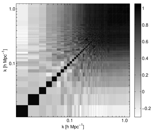
Figure 3: Correlation matrix (Equation 13) at $z=0.5$ produced by averaging 1000 simulation power spectra as shown in Figure 2. The dark points on the diagonal and at the large-$k$ regime indicate positive correlation, as we expected. As described in Section 5, this figure shows a binning independent version of the correlation matrix.

Figure 4: The ratio between the diagonal components of the non-Gaussian ($C_{ii}$) and Gaussian ($(C_{g})_{ii}$) covariance matrices, at $z=0.5$. For $C_{g}$ we evaluated in 2 ways. Using Equation 14, the $P(k)$ can either be averaged over our set of simulations, or simply computed from linear theory using CAMB. For either case, this plot shows that even the diagonal components of the non-Gaussian covariance matrix are not Gaussian, as the ratio clearly departs from unity with higher $k$. The sharp increase at $k\sim 0.5\ \mathrm{Mpc}^{-1}h$ is caused by the logarithmic binning, in which each bin suddenly accumulates the departure contributions from many more Fourier modes. As we will justify in the results discussion later, we do not consider modes where $k>0.5$ Mpc${}^{-1}h$.

4.3 Fisher information function

As previously considered by Rimes & Hamilton (2005, 2006), a useful quantity that can be derived from the covariance matrix is the cumulative Fisher information function

$$I(k_{j})=\sum^{k_{j}}_{k,k^{\prime}}C_{norm}^{-1}(k,k^{\prime})$$ (15)

where $C_{norm}$ is the $j\times j$ sub-matrix of $C(k,k^{\prime})$ (or $C_{g}$) with $k,k^{\prime}\leq k_{j}$, further normalized by $\langle P(k)\rangle\langle P(k^{\prime})\rangle$. In other words,

$$C_{norm}(k,k^{\prime})=\frac{C(k,k^{\prime})}{\langle P(k)\rangle\langle P(k^{\prime})\rangle}\qquad(k,k^{\prime}\leq k_{j}\ \mathrm{only}).$$ (16)

Here $I(k)$ describes the information contained in the amplitude of the power spectrum up to a scale $k$. Although the form of $I(k)$ seems like a mathematical contrivance, it indeed has physical significance in weak lensing (Lu et al, 2010).

Figure 5 shows the Fisher information function using our set of simulations. It also compares the information that can be obtained by a Gaussian and a non-Gaussian covariance matrix. At small $k$, gravity is still linear, so the non-Gaussian information is similar to the Gaussian case, as also seen in Figure 3. At $k\gtrsim 0.3\ \mathrm{Mpc}^{-1}h$, however, the information flattens out into a so-called “trans-linear plateau”, which is consistent with previous studies by Rimes & Hamilton (2005) and Takahashi et al (2011). This corresponds to the scale where the $k$ modes become correlated.

Qualitatively, the Fisher information function tells us how much information can be extracted from a given $k$ mode. At small $k$, each mode is independent, so more information can be extracted by measuring more modes. At large $k$, the Fisher information function flattens, meaning very little information can be extracted by measuring extra modes. Indeed, as seen from Figure 5, one can extract orders of magnitude more information when using a Gaussian covariance matrix instead of the true covariance matrix. This information, however, does not exist in the data. Consequently, an analysis using a Gaussian estimator would most likely underestimate the error bars for any measurements beyond the trans-linear scale ($k\gtrsim 0.3\ \mathrm{Mpc}^{-1}h$).

Before proceeding to the construction of the Fisher matrix and of the three estimators, we reduce the noise that exists in our covariance matrices, as described in the following section.

Figure 5: Top panel: Cumulative information (Equation 15) per unit volume at $z=0.5$. The filled circles were obtained by using both the reconstructed power spectrum and the reconstructed covariance matrix in Equation 16. Bottom panel: Same plots as the top, but with different binning schemes to show that the plateau of information is not a binning artifact. Similar plots can also be found in Rimes & Hamilton (2005, 2006).

5 Noise reduction

As mentioned in the introduction, to achieve convergence on the $N^{2}$ elements of the covariance matrix is not an easy task. Among the possible approaches, the brute force way (i.e. running a very large number of N-body simulations) is probably the least affordable in terms of computational resources. In this section, we apply a noise reduction technique that reduces to $2N$ the number of elements one needs to extract.

Our technique is based on the assumption that the cross-correlation coefficient matrix (see Figure 3) can be parameterized as the sum of a diagonal and off-diagonal components, and we put a strong prior on the latter: it must be expressed as a sum over the outer products of the principal Eigenvectors. The diagonal component is then simply obtained such as each diagonal element in the final matrix is equal to 1.

To extract the Eigenvectors, we perform an iterative eigenvalue decomposition of the off-diagonal component and keep only the dominant terms. We start by modeling the full matrix as the sum of an identity matrix $\delta_{k,k^{\prime}}$ and an off-diagonal component, from which we extract the largest eigenvalue $\lambda$ and Eigenvector $U_{\lambda}(k)$. At the next iteration step, we model the diagonal component as $\delta_{k,k^{\prime}}(1-\lambda U_{\lambda}^{2}(k))$, subtract that quantity from the original matrix, and extract the principal Eigenvector of the result. We repeat this process until the difference between the original and the model converges – four times in this case. At the end of the iterative step $i$, the parameterized matrix is thus given by

$$\rho^{i}(k,k^{\prime})=\delta_{k,k^{\prime}}\left(1-\lambda^{i-1}[U_{\lambda}^{i-1}(k)]^{2}\right)+\lambda^{i}U_{\lambda}^{i}(k)U_{\lambda}^{i}(k^{\prime})$$ (17)

After the last iteration, we update the first term with the latest $\lambda$ and $U_{\lambda}(k)$. The diagonal component typically starts off as unity in the largest scales and fades away in the non-linear regime. In this case, the strongest eigenvalue is almost two orders of magnitude larger than all others, hence we keep only a single Eigenvector (see (Harnois-Deraps & Pen, 2011) for the application of this method when the angular dependence of the covariance matrix is preserved).

The modeled covariance matrix is then recovered from this noise-reduced cross-correlation matrix with the diagonal elements of the original covariance $C(k,k)$ (not to be confused with the diagonal component of the factorization of $\rho(k,k^{\prime})$) following Equation 13. Although we do need $N^{2}$ matrix elements to start with, the power of this decomposition relies on the fact that the prior is accurate at the few percent level, and that everything that does not fit into this form is considered as noise. We thus recover smooth and accurate covariance matrices, even though the input elements are noisy. The explanation for this is that one needs only to measure the N diagonal elements of the covariance matrix (which are generally the easiest to resolve) plus one Eigenvector (which combines the data of a large portion of the matrix into another N elements).

We present the fractional error between the modeled and the original matrices in Figure 6, and observe that individual elements match the model at the ten percent level at $k\sim 0.2\ \mathrm{Mpc}^{-1}h$. This improves to the few percent level for even smaller scales. We expect these higher $k$ modes to be more accurately measured to start with, since they come from the angle averaging of $k$-shells that contain much larger number of cells.

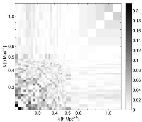
Figure 6: Absolute value of the fractional error between the modeled covariance matrix and the original, from unreconstructed density fields at $z=0.5$. As expected, the lower $k$ modes are more noisy due to lower statistics. We still achieve an agreement of about ten percent at $k\sim 0.22\ \mathrm{Mpc}^{-1}h$, and even better for smaller scales.

Figure 7: The ratio of the diagonals to the Gaussian approximation. The squares are from the original matrix, the open circles are from the diagonal component of the factorization, and the stars are from the diagonal of the off-diagonal contribution. The diagonal component is closer to the Gaussian prediction down to much smaller scales, as most of the non-Gaussianities are factorized in the other term.

We then present in Figure 7 the diagonals of the original covariance matrix and of both components, divided by the Gaussian prediction. The sum of the two components is equal to the original matrix on the diagonal by construction. The off-diagonal components of the factorization can be tested against the original by comparing the cumulative Fisher informations (Equation 15). We observe that the information from the factorized covariance matrices exhibit the same essential features, namely a Gaussian increase up to about $k\sim 0.2\ \mathrm{Mpc}^{-1}h$, followed by a saturation plateau. We present the ratio of this modeled information to the original distribution in Figure 8 and observe that the factorization reproduces the information content at the few percent level. Although the figures presented in this section correspond to the unreconstructed densities at $z=0.5$, we achieve comparable performances on reconstructed density fields at all measured redshifts.

Figure 8: The ratio between the Fisher information of our modeled covariance matrix and that of the original, from unreconstructed density fields at $z=0.5$. The departure from the original is at most $10\%$, and the agreement is otherwise at the few percent level.

This factorization has one extra advantage, which comes from the fact that $U(k)\sqrt{C(k,k)}$ is binning independent. The original covariance matrix is binning dependent, since the number of modes entering each element varies as we change from linear to logarithmic bands, for example. This is correct, but it has a major inconvenience – the cross-correlation coefficient matrix (Equation 12) visually changes significantly. It becomes a tedious task to compare figures from different authors. We can therefore attempt to fix this problem by constructing binning independent quantities.

The diagonal component, $1-\lambda U^{2}(k)$, is close to Gaussian, as seen in Figure 7, hence it is roughly inversely proportional to the number of modes in the bin. We scale it with the ratio between the measured number of modes and the continuous limit case: $N_{cont}\sim 4/3\pi(k/k_{min})^{3}$, and obtain a binning independent quantity. We have also shown in this section that the off-diagonal elements of the covariance matrix are well modeled by $\lambda U(k)U(k^{\prime})\sqrt{C(k,k)C(k^{\prime},k^{\prime})}$, which are binning independent as well. The solution is thus to replace the diagonal of the original covariance matrix such that

$$C(k,k)\rightarrow\left[1-\lambda U^{2}(k)\right]\frac{N}{N_{cont}}+\lambda U^{2}(k).$$ (18)

This bin independent result is made available thanks to the factorization presented above, which allows us to isolate the bin dependence (that comes exclusively from the diagonal component) and to apply our correction. The cross-correlation coefficient matrix calculated that way is shown in Figure 3, and compares well with Rimes & Hamilton (2005), apart from the anti-correlation between the largest and the smallest modes (see section 4.2, and note that it is not clear that the simulations Rimes & Hamilton (2005) were large enough to contradict our anti-correlation result).

6 Parameter estimation

6.1 Optimal estimator

For a set of parameters $p_{i}$, the Fisher matrix $F_{ij}$ is given by the inverse of a covariance matrix

$$F_{ij}=C_{ij}^{-1}$$ (19)

where $C_{ij}\equiv C(k_{i},k_{j})$ or $C_{g}$, as described in the previous sections. Since our $C_{ij}$ is derived from power spectra, the parameters in $F_{ij}$ can be thought of as the power for each $k$ mode in the power spectrum. To obtain the Fisher matrix for another set of parameters $q_{\mu}$, we can project the power spectrum Fisher matrix onto the new parameter space using

$$F_{\alpha\beta}=\sum_{k_{i},k_{j}}^{k_{max}}\frac{\partial P(k_{i})}{\partial q_{\alpha}}F_{ij}\frac{\partial P(k_{j})}{\partial q_{\beta}}.$$ (20)

Using $F_{\alpha\beta}$, the optimal error estimator for parameter $q_{\alpha}$ is simply

$$\Delta q_{\alpha}=\left(F^{-1}\right)_{\alpha\alpha}^{1/2}.$$ (21)

The estimators for cases (ii) and (iii) are obtained from substituting Equations 12 and 14 respectively in Equation 19.

For our purposes, since we are interested in estimating the fractional errors of $s$ (1D) or $s_{\perp}$ and $s_{||}$ (2D), we set $q\equiv\ln s$ in 1D, and $q_{1}\equiv\ln s_{\perp}$ and $q_{2}\equiv\ln s_{||}$ in 2D. The derivatives in Equation 20 can be evaluated in a number of ways. We can either produce a variety of $P(k)$ using different parameters $s$ and take their finite differences, or we can parametrize $P(k)$ as a function of $s$, and evaluate the derivatives analytically. In both cases, we decompose the power spectrum into a smooth component and a wiggly component

$$P(k)=P_{smooth}(k)+P_{wiggle}(k).$$ (22)

When using BAO to measure distances, all information is manifested as “wiggles” in the power spectrum. To ensure that all our measurements originate from BAO, we subtract $P_{smooth}(k)$ (Eisenstein & Hu, 1998) from our full $P(k)$ prior to taking derivatives. For the rest of this paper, we refer $P_{wiggle}(k)$ and $dP_{wiggle}/dx$ to simply $P(k)$ and $dP/dx$ for brevity.

The finite differencing of $P(k)$ is done by producing many $P(k)$ using CMBFAST, and dividing their differences by the differences of $s$ being used. On the other hand, readers familiar with Seo & Eisenstein (2007) would recall that they suggested an analytical form of the wiggles using a damped sync function, and they approximated the square of the sinusoidal components in the Fisher matrix as a constant. In our work, since we use non-Gaussian (hence non-diagonal) covariance matrices, we do not adapt that constant approximation, as the detailed structure of the signal becomes important once off-diagonal errors are present. Nevertheless, it is interesting to show what effect this approximation and the off-diagonal elements of the covariance matrix can have on our results. See Appendix A for this discussion.

6.2 Sub-optimal estimator

In a data analysis, non-linear covariance matrices are usually hard to measure with a high signal to noise, especially in surveys that exhibit complex selection functions. What is often done in that case is to assume Gaussianity in the data, while ignoring the fact that the band powers themselves are actually non-Gaussian. The values extracted for the mean and the error on the BAO dilation scale are not properly weighted, since they assume that all errors in $k-$bands are uncorrelated. As mentioned earlier, the resulting mean is sub-optimal, while the error bars are most likely off by an unknown amount. Since we now have measured a non-linear covariance matrix $C$, we are in a position to compare the correct error bars for existing data analysis (case (i)) with those quoted in literature, which approach case (iii) at various levels. We recall that the difference between sub-optimal and optimal is somewhat reduced for analyses that model the non-linearities in the fields.

We derive a “sub-optimal” estimator by solving the linear system $Ax=b$ where $x$ is a vector containing a set of cosmological parameters of interest (here we consider only $x\equiv\Delta\ln s$, hence $x$ is a scalar, but this method could be generalized to include $\ln s_{\perp}$ and $\ln s_{||}$ for instance), and $b$ is a noisy observable, associated with a noisy covariance matrix $\tilde{C}$. In our case, the observable under study is $\Delta P(k)$, the deviation from the mean of the power spectrum. With this correspondence, we get $A\equiv\partial{P(k)}/\partial\ln s$ – a vector in our case. To estimate each component of $x$, we first weight each observed point by the inverse of the covariance matrix associated with the observation of $b$, i.e. $\tilde{C}$, and then proceed to solve for $x$ by taking pseudo-inverses such that

$$x=(A^{T}\tilde{C}^{-1}A)^{-1}A^{T}\tilde{C}^{-1}b.$$ (23)

Finally, the errors on the elements of $x$ are given by the diagonal components of the covariance matrix $\langle x^{2}\rangle=xx^{T}$. We obtain the following estimator for the error in $\ln s$:

$$\langle(\Delta\ln s)^{2}\rangle=(P_{s}^{T}\tilde{C}^{-1}P_{s})^{-1}P_{s}^{T}\tilde{C}^{-1}C\tilde{C}^{-1}P_{s}(P_{s}^{T}\tilde{C}^{-1}P_{s})^{-1}$$ (24)

where $P_{s}\equiv\partial{P}/\partial\ln s$, and $P_{s}^{T}CP_{s}$ is a vector-matrix-vector product similar to Equation 20, and where $C=bb^{T}$ is the improved estimate of the non-linear covariance matrix, which we obtained from our simulations. Notice that if the true covariance matrix was indeed Gaussian (i.e. $C=\tilde{C}=C_{g}$), we would recover the optimal estimator where $\langle(\Delta\ln s)^{2}\rangle=(P_{s}^{T}C_{g}^{-1}P_{s})^{-1}=F_{11}^{-1}$. In other words, cases (i), (ii), and (iii) would be identical. Conversely, if the original matrix was already the optimal measurement (i.e. $C=\tilde{C}$), we would get $\langle(\Delta\ln s)^{2}\rangle=(P_{s}^{T}C^{-1}P_{s})^{-1}$, i.e. cases (i) and case (ii) would be the same, possibly different from case (iii). We also note that the inverse of the true covariance matrix is not involved in Equation 24.

In the next sections, we consider the case where Gaussianity was originally assumed in a BAO analysis, we correctly estimate the error of $x$ (with this sub-optimal estimator) and compare the results produced with an optimal estimator.

6.3 Effects of reconstruction

As seen in Figure 1, density reconstruction sharpens the acoustic peak in the correlation function. This is equivalent to reducing the non-linear damping of the wiggles in the power spectrum. We parametrize the reduction of damping due to reconstruction by an extra factor in front of $\Sigma_{nl}$ in the damping factor (Seo & Eisenstein, 2007) such that

$$\exp\left[-\frac{k^{2}\Sigma_{nl}^{2}}{2}\right]\rightarrow\exp\left[-\frac{(1-f)^{2}k^{2}\Sigma_{nl}^{2}}{2}\right]$$ (25)

where $f=1$ represents 100% reconstruction, canceling any non-linear effects. In reality, such a case is unachievable, as some information has been irreversibly lost. In principle, we could measure $f$ by extracting the power spectrum wiggles before and after reconstruction, and find the best fit damping factor. Looking at Figure 1, we see that the reconstructed correlation at $z=0.5$ is very similar to the correlation at $z=2$. The ratio of growth factors between these two redshifts is 0.55, and the reconstructed field actually looks slightly better than the $z=2$ field, so we adopt the standard $f=0.5$, which reduces non-linear damping by 50% (Seo & Eisenstein, 2007; Masui et al, 2010).

7 Results and discussion

We set up hypothetical surveys with volume $V=(1\ h^{-1}\mathrm{Gpc})^{3}$ centered on redshifts $z=0.5$ and $z=1.0$. We then produce fractional distance errors $\Delta s/s$ using the three aforementioned estimators:

• Sub-optimal estimator (Equation 24)

• Optimal estimator (Equation 21) with a non-Gaussian covariance matrix (Equation 12),

• Optimal estimator (Equation 21) with a Gaussian covariance matrix (Equation 14).

The distance error measurements use only the information up to a limiting $k_{max}$ in the covariance matrix; all $k>k_{max}$ are marginalized over (i.e. cut off from the covariance matrix before it is inverted). For each error estimate, we also produce bootstrap error bars to show the convergence of our set of 1000 simulations. This is done by picking 1000 random simulations (allowing repeats) from our set, and taking the standard deviations of the results using 2000 such random sets. The noise reduction technique is performed for every set.

The only redshift dependence in the estimator comes from the non-linear damping scale $\Sigma_{nl}(z)$ (Equation 25). In addition, we know from Figures 3 and 5 that the covariance matrices in the linear regime are similar to the Gaussian covariance matrix. Therefore, we expect errors at small $k$ to be hardly distinguishable among estimators and redshifts. At large $k$, however, we expect the effects of the covariance matrices and the derivatives to have a more pronounced effect on the estimator. The redshift dependent damping scale $\Sigma_{nl}(z)$ becomes important and distinguishes between $z=0.5$ and $z=1.0$.

The top panels of Figures 9 and 10 show the measured distance errors vs limiting $k_{max}$, with and without reconstruction, respectively. The bottom panels shows the squares of the ratio of cases (i) and (ii) to case (iii) from the top plot at $z=0.5$. In all scenarios, we consider only the modes $k\lesssim 0.5$ Mpc${}^{-1}h$ where our simulations remain reliable (Figure 2). Moreover, we do not expect modes of $k>0.5$ Mpc${}^{-1}h$ to carry any BAO information, as the wiggles on small scales suffer from Silk damping (Eisenstein & Hu, 1998) as well as non-linear damping (Section 6.3).

Figure 10 shows the distance errors with $f=0.5$ and covariance matrices from reconstructed simulations. Since some of the wiggles are indeed recovered, the optimal distance errors decreased by 50% to 70% compared to the case with no reconstruction (Figure 9). More importantly, though, the discrepancy between sub-optimal and optimal estimates becomes slightly more severe. In the presence of reconstruction, a naive Gaussian assumption can underestimate the variance of the errors by up to 20% near the trans-linear scales ($k\sim 0.2$ Mpc${}^{-1}h$). Somewhat disturbingly, at small scales $k>0.5$ Mpc${}^{-1}h$ the sub-optimal estimate deviate significantly from the optimal estimate. A sub-optimal estimator certainly is not expected to provide the same result as an optimal estimator. And also, as mentioned above, the regime $k>0.5$ Mpc${}^{-1}h$ is irrelevant to BAO analysis. Therefore, we did not investigate this behavior further.

Our results from Figure 9 show that the three treatments of the errors have similar constraining power on the BAO dilation scale. This conclusion is consistent with that from Takahashi et al (2011), which measured that cases (ii) and (iii) give almost identical results, without reconstruction. However, we push the envelope further and show that, first, the sub-optimal estimator also behaves similarly, with deviations by up to $15\%$. Second, we show that the reconstruction of density fields improves the constraints on dilation by about 70% at $z=0.5$. The improvement is more modest at higher redshifts, where additional BAO peaks are still in the linear regime. Third, we conclude that with reconstruction, Gaussian assumption can underestimate the errors on the dilation scale in a similar level to the case without reconstruction.

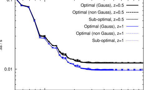
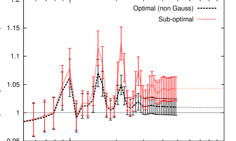
Figure 9: Top panel: Fractional distance errors using optimal and sub-optimal estimators, without reconstruction. Optimal (Gauss) and Optimal (non Gauss) denote Fisher estimators from covariance matrices $C_{g}$ and $C$ respectively. Sub-optimal denotes the correct non-Gaussian errors if Gaussianity was assumed. The error bars on each line are the 1-$\sigma$ bootstrap error bars for the statistical fluctuations in our set of simulations. Middle panel: Optimal non-Gaussian and sub-optimal errors, each divided by the optimal Gaussian errors at $z=0.5$. This panel shows that each error estimate deviates by only a few percent from the Gaussian estimate. Bottom panel: Our $dP/ds$ template which shows that the regime $k>0.5$ Mpc${}^{-1}h$ is no longer relevant for BAO analysis, as the wiggles are mostly damped and converged to zero.

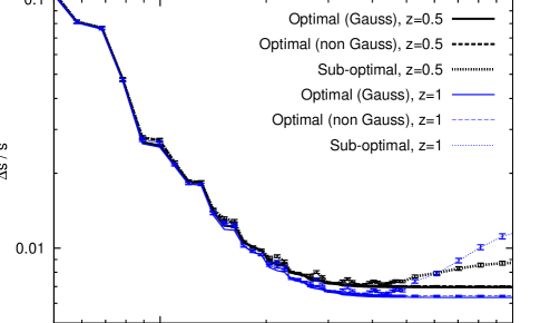
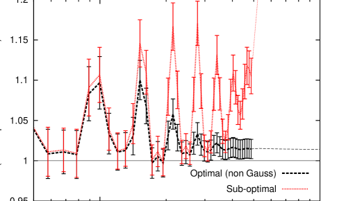
Figure 10: Fractional distance errors after reconstruction. Compared to Figure 9, this now includes reconstructed covariance matrices and a reconstruction factor of $f=0.5$. In the sub-optimal case, the increase at the regime $k>0.5$ Mpc${}^{-1}h$ is a statistical curiosity, but irrelevant for a BAO analysis. We base our conclusion on the values for $k\lesssim 0.5$ Mpc${}^{-1}h$. This cut-off coincides with our choice to switch from linear binning to logarithmic binning, but we have checked that the above plots contain no binning artifacts.

8 Conclusion

We have addressed some aspects of the problem of measuring non-Gaussian error bars in a BAO analysis. We have investigated the full optimal quadratic non-Gaussian estimator on reconstructed density field, and quantified the significance of the non-Gaussianities on the BAO dilation scale error. A major subtlety is that the optimal estimator requires an accurate measurement of the inverse of the covariance matrix of power spectrum, and the actual uncertainty on that inverse had never been measured. The accuracy of the inverse is generally bin dependent, and convergence requires a large number of N-body simulations. We have overcome this problem with a factorization technique that involves an iterative eigenvalue decomposition of the covariance matrix, which we measured from 1000 N-body simulations. We further measured the uncertainty of the inverse of the matrix with bootstrap re-sampling, and were able to achieve convergence at the percent level.

Having confidence in the inverse matrix, we quantitatively compared the measurement of the error on the BAO dilation factor obtained with different estimators. We construct an optimal estimator, which gives the most accurate measurement of the error achievable on the BAO dilation scale. It is derived from a covariance weighted Fisher matrix, which is constructed out of the inverse of the non-linear power spectrum covariance matrix. We compared our results with those obtained from the purely Gaussian forecast, and we measure significant discrepancies of up to ten percent in the error on the dilation scale.

We also measured non-Gaussian error bars on the mean BAO dilation scale that has been obtained with a Gaussian estimator, as is usually encountered in the literature. Because we have confidence in the accuracy of our covariance matrix, this sub-optimal estimator provides a robust estimate of the error bars on the BAO dilation scale. To illustrate our point, we considered the case where the original dilation scale was measured under standard Gaussian statistics. We found that the variances of those measurements can differ by up to 15%, compared to our optimal estimator. Many data analyses did include non-Gaussianities in their BAO error estimator, hence the discrepancy between these and our optimal estimator is likely to be more modest than that obtained in this work.

We note in passing that these results were entirely obtained from N-body simulations, hence the effect of the survey selection function has been factored out of our problem. Constructing optimal estimators with actual data will however be more challenging, since it has to include such an effect, which effectively couple Fourier modes from different bins, in addition to account for the effect of bias between the sampled tracers (i.e. galaxies or 21cm structure) and the underlying matter density.

We have also implemented a density reconstruction algorithm, which recovers some of the lost BAO information due to non-linear gravitational collapse at late times. In that case, the error on the dilation scale is reduced by a factor of about 70% at low redshift, but the discrepancy between the sub-optimal and optimal estimates remains similar to the case without reconstruction (20% and 15%, with and without reconstruction).

We mention in conclusion that in a survey, the increase in variance we observed when using a sub-optimal estimator is equivalent to losing about the same percentage of survey volume, because the variance of measurements is inversely proportional to volume. These discrepancies should be taken seriously into account especially when forecasting performances of future telescopes, where the objective is to reach percent level precision on cosmological parameters.

Appendix A Power spectrum derivative

Interestingly even though the Fisher information (Figure 5) of Gaussian and non-Gaussian covariance matrices differ by about an order of magnitude near $k\gtrsim 0.2$ Mpc${}^{-1}h$, the measurement errors (Figures 9 and 10) differ by only a few percent. The reason for this is that when the oscillatory power spectrum derivative $dP/d\ln s$ is multiplied into the covariance matrix to compute the Fisher matrix (Equation 20), the off-diagonal elements of the covariance matrix can be canceled out.

In Seo & Eisenstein (2007), they considered the regime $k\gtrsim 0.05$ Mpc${}^{-1}h$ and approximated a $\cos^{2}(ks)$ term, which originates from $dP/d\ln s$, as simply $1/2$ without any oscillations when computing their Fisher matrix. Since we are considering a similar regime, we also attempted this approximation. We emphasize that this approximation is not applicable to us, as our non-Gaussian covariance matrix is not diagonal. Nevertheless, it illustrates the effect that an oscillatory $dP/d\ln s$ can have on distance measurements.

Figure 11 shows $\Delta s/s$ as a function of limiting $k_{max}$, using the approximated derivative. This can be compared to the top panel in Figure 9, where the only difference is that Figure 11 uses the approximated $dP/d\ln s$, and Figure 9 computes $dP/d\ln s$ by finite differences of actual power spectra. In both figures, the optimal estimators follow the inverse of the Fisher information (Equation 15). For the optimal Gaussian case, the errors using either forms of derivatives give similar results (other than some oscillations at small $k$). This is expected since the Gaussian covariance matrix is diagonal (Equation 14), so the approximation is valid. For the sub-optimal cases we considered in this paper, however, the discrepancies from the optimal Gaussian case reach factors of 2 to 3, depending on redshift. This can be attributed to the fact that all elements of the covariance matrix are given a uniform weight. When using the finite difference derivatives, however, different elements are weighted according to the values of $dP/d\ln s$ at their corresponding $k$ modes. This effectively cancels most of the contributions from the off-diagonal elements of the covariance matrix, which explains why the optimal and sub-optimal errors differ by only a few percent in that case.

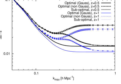
Figure 11: Fractional distance errors using various estimators, similar to the top panel of Figure 9 (without reconstruction). The only difference here is that the power spectrum derivative in the Fisher matrix is an approximation which does not oscillate. Compared to Figure 9, the Optimal (Gauss) case is similar, but the other cases are clearly different.

References

- Bassett & Hlozek (2009) Bassett B.A., Hlozek R., 2009, in Ruiz-Lapuente P., ed., Dark Energy, Cambridge University Press, New York.
- Blake & Glazebrook (2003) Blake C., Glazebrook K., 2003, ApJ, 363, 1329.
- Blake et al (2010) Blake C., et al, 2010, MNRAS, 406, 803.
- Cole et al (2005) Cole S., Percival W., et al., 2005, MNRAS, 362, 505.
- Coles & Jones (1991) Coles P., Jones B., 1991, MNRAS, 248, 1.
- Eisenstein & Hu (1998) Eisenstein D.J., Hu W., 1998, ApJ, 496, 605.
- Eisenstein (2005) Eisenstein D.J., 2005, New Astronomy Reviews, 49, 360.
- Eisenstein et al (2005) Eisenstein D.J., Zehavi I., et al., 2005, ApJ, 633, 560.
- Eisenstein et al (2007) Eisenstein D.J., Seo H.J., Sirko E., Spergel D.N., 2007, ApJ, 664, 675.
- Feldman et al (1994) Feldman H., Kaiser N., Peacock J., 1994, ApJ, 426, 23.
- Goldberg (2000) Goldberg D., 2000, PhD thesis, Princeton University.
- Guth (2004) Guth A., 2004, in Carnegie Observatories Astrophysics Series, Vol. 2: Measuring and Modeling the Universe, Cambridge University Press, New York.
- Harnois-Deraps & Pen (2011) Harnois-Déraps J., Pen U.-L., 2011, MNRAS submitted. (arXiv:1109.5746)
- Hockney & Eastwood (1980) Hockney R.W., Eastwood J.W., 1980, Computer Simulation Using Particles. Taylor & Francis Group, New York.
- Hütsi (2006) Hütsi, G., 2006, Astron. Astrophys., 449, 891.
- Lu et al (2010) Lu T., Pen U.-L., Doré O., 2010, Phys Rev D, 81, 123015.
- Masui et al (2010) Masui, K.W., McDonald P., Pen U.-L., 2010, Phys Rev D, 81, 103527.
- McDonald & Eisenstein (2007) McDonald P, Eisenstein D.J., 2007, Phys. Rev. D 76, 063009.
- Merz et al (2005) Merz H., Pen U.-L., Trac H., 2005, New Astron, 10, 393.
- Meiksin & White (1999) Meiksin, A., White, S., 1999, MNRAS, 308, 1179.
- Miller et al (1999) Miller A.D., Caldwell R., et al., 1999, ApJ, 524, L1.
- Neyrinck et al (2009) Neyrinck M., Szapudi I., Szalay A., Astrophys. J. Let. 698 (2009) L90-L93.
- Noh et al (2009) Noh Y., White M., Padmanabhan N., 2009, Phys Rev D, 80, 123501.
- Padmanabhan et al (2009) Padmanabhan N., White M., Cohn J.D., 2009, Phys Rev D, 79, 063523.
- Percival et al (2001) Percival W., Baugh C., et al., 2001, MNRAS, 327, 1297.
- Percival et al (2010) Percival W., Beth R., et al., 2010, MNRAS, 401, 2148.
- Rimes & Hamilton (2005) Rimes C.D., Hamilton A.J.S., 2005, MNRAS, 360, L82.
- Rimes & Hamilton (2006) Rimes C.D., Hamilton A.J.S., 2006, MNRAS, 371, 1205.
- Scoccimarro et al (1999) Scoccimarro, R., Zaldarriaga, M., Hui, L., 1999, ApJ, 527, 1.
- Seo & Eisenstein (2003) Seo H.J., Eisenstein D.J., 2003, ApJ, 598, 720.
- Seo & Eisenstein (2005) Seo H.J., Eisenstein D.J., 2005, ApJ, 633, 575.
- Seo & Eisenstein (2007) Seo H.J., Eisenstein D.J., 2007, ApJ, 665, 14.
- Seo et al (2010) Seo H.J., Eckel J., Eisenstein D.J., et al., 2010, ApJ, 720, 1650.
- Seo et al (2011) Seo H.J., Masanori S., Dodelson S., Jain B., Takada M., 2011, ApJ, 729, L11.
- Smith et al (2003) Smith R.E., Peacock J.A., Jenkins A., et al., 2003, MNRAS, 341, 1311.
- Takahashi et al (2009) Takahashi R., Yoshida N., Takada M., et al., 2009, ApJ, 700, 479.
- Takahashi et al (2011) Takahashi R., Yoshida N., Takada M., et al., 2011, ApJ, 726, 7.
- Tegmark (1997) Tegmark M., 1997, Phys Rev Lett, 79, 3806.
- Tegmark et al (2006) Tegmark M., Eisenstein M., et al., 2006, Phys Rev D, 74, 123507.
- Yu et al (2010) Yu H.-R., Harnois-Déraps, J., Zhang T.-J., Pen U.-L., 2010, ApJ submitted. (arXiv:1012.0444)
- Zel’Dovich (1970) Zel’Dovich, Y.B., 1970, Astron. Astrophys., 5, 84.
- Zhang et al (2010a) Zhang T.-J., Yu H.-R., Harnois-Déraps J., MacDonald I., Pen U.-L., 2011, ApJ, 728, 35.