Abstract

Exit times for stochastic Ginzburg-Landau classical field theories with two or more coupled classical fields depend on the interval length on which the fields are defined, the potential in which the fields deterministically evolve, and the relative stiffness of the fields themselves. The latter is of particular importance in that physical applications will generally require different relative stiffnesses, but the effect of varying field stiffnesses has not heretofore been studied. In this paper, we explore the complete phase diagram of escape times as they depend on the various problem parameters. In addition to finding a transition in escape rates as the relative stiffness varies, we also observe a critical slowing down of the string method algorithm as criticality is approached.

Lan Gong1 and D. L. Stein1,2

lan.gong@nyu.edu   daniel.stein@nyu.edu

1Department of Physics, New York University, New York, NY 10003

2Courant Institute of Mathematical Sciences, New York University, New York, NY 10003

1 Introduction

In a previous paper [1] (hereafter GS), the authors introduced and solved a system of two coupled nonlinear stochastic partial differential equations. Such equations are useful for modelling noise-induced activation processes of spatially varying systems with multiple basins of attraction. Examples of such processes include micromagnetic domain reversal [2, 3], pattern nucleation [4, 5, 6], transitions in hydrogen-bonded ferroelectrics [7], dislocation motion across Peierls barriers [8], and structural transitions in monovalent metallic nanowires [9, 10]. It is the last problem in particular that the model introduced in GS was constructed to analyze.

The GS model provided a mathematical realization of a stochastic Ginzburg-Landau field theory consisting of two coupled classical fields, denoted $\phi_{1}(z)$ and $\phi_{2}(z)$, defined on a linear domain of finite extent $L$. Stochastic partial differential equations of this type are constructed to model noise-driven transitions between locally stable states. In the especially important case of weak noise, where the transition rate is of the Arrhenius form $\Gamma_{0}e^{-\Delta E/\epsilon}$, with prefactor $\Gamma_{0}$ and activation barrier $\Delta E$ independent of the noise $\epsilon$, the transition path occurs near (i.e., within a lengthscale of order $O(\epsilon^{1/2})$) the saddle (or col) of least action connecting the two stable states.

The two-field model displayed several interesting features, including a type of “phase transition” in activation behavior as $L$ varied. The transition was driven by a change in the saddle state, from a uniform configuration at small $L$ to a spatially varying one (“instanton”) at larger $L$. This transition has been noticed and analyzed for the case of a single field [11, 12], but had not been seen in the rarely studied case of a system with two coupled fields. Perhaps more remarkably, the system admitted an exact solution for the instanton state; such exact solutions are rare in the case of nonlinear field theories with a single field, much less a nontrivial system of coupled fields.

The introduction of two fields was required to study transitions among different quantized conductance states in non-axisymmetric nanowires. The axisymmetric case had previously been treated theoretically in [13, 9]. However, detailed studies using linear stability analysis by Urban et al. [14] indicated that roughly 1/4 of all such transitions involved either non-axisymmetric initial or final states, or else a least-action transition passing through a non-axisymmetric saddle. To describe such transitions, one field ($\phi_{1}(z)$) describes radial variations along the wire length and the other ($\phi_{2}(z)$) describes deviations from axisymmetry.

One restriction of the analysis in GS was that the respective bending coefficients $\kappa_{1}$ and $\kappa_{2}$ of the two fields were taken to be equal. However, this is generally not the case in real nanowires [14]. Therefore, in order to apply the model to actual transitions, as well as to provide a complete picture of the activation behavior in such systems, we need to consider the case where $\kappa_{1}\neq\kappa_{2}$. In such cases analytical solutions cannot be found and we need to rely on numerical methods. The study of this more general problem is the subject of this paper.

2 The Model

Consider two coupled classical fields $\phi_{1}(z)$, $\phi_{2}(z)$ on the interval $[-L/2,L/2]$, subject to the energy functional

$${\cal H}=\int_{-L/2}^{L/2}\!(\frac{1}{2}\kappa_{1}(\phi_{1}^{\prime}(z))^{2}+\frac{1}{2}\kappa_{2}(\phi_{2}^{\prime}(z))^{2}+U(\phi_{1},\phi_{2}))\,dz\,.$$ (1)

where

$$U(\phi_{1},\phi_{2})=-\frac{\mu_{1}}{2}\phi_{1}^{2}+\frac{1}{4}\phi_{1}^{4}-\frac{\mu_{2}}{2}\phi_{2}^{2}+\frac{1}{4}\phi_{2}^{4}+\frac{1}{2}\phi_{1}^{2}\phi_{2}^{2}$$ (2)

The bending coefficients $\kappa_{1}$, $\kappa_{2}$ can be related to the wire surface tension [13, 9]. The arbitrary positive constants $\mu_{1}$, $\mu_{2}$ are chosen such that $\mu_{1}\neq\mu_{2}$, breaking rotational symmetry. (The case $\mu_{1}=\mu_{2}$ has been investigated analytically by Tarlie et al. [15] in the context of phase slippage in conventional superconductors.)

If the system is subject to additive spatiotemporal white noise, then their time evolution is governed by the pair of stochastic partial differential equations:

$$\dot{\phi_{1}}=\kappa_{1}\phi_{1}^{\prime\prime}+\mu_{1}\phi_{1}-\phi_{1}^{3}-\phi_{1}\phi_{2}^{2}+\sqrt{2\epsilon}\,\xi_{1}(z,t)$$

$$\dot{\phi_{2}}=\kappa_{2}\phi_{2}^{\prime\prime}+\mu_{2}\phi_{2}-\phi_{2}^{3}-\phi_{1}^{2}\phi_{2}+\sqrt{2\epsilon}\,\xi_{2}(z,t)\,,$$ (3)

where $\xi_{1,2}$ are the spatiotemporal noise terms satisfying $<\xi_{i}(z_{1},t_{1})\xi_{j}(z_{2},t_{2})>=\delta(z_{1}-z_{2})\delta(t_{1}-t_{2})\delta_{ij},~{}i,j=1,2$. If the noise is due to thermal fluctuations, then by the fluctuation-dissipation theorem $\epsilon=k_{B}T$.

The activation energy $\Delta E$ and prefactor $\Gamma_{0}$ in the Arrhenius rate formula depend not only on the details of the potential (2), but also on the interval length $L$ on which the fields are defined, and on the choice of boundary conditions at the endpoints $z=-L/2$ and $z=L/2$. It was shown in [16] that Neumann boundary conditions are appropriate for the nanowire problem, and we will employ them here.

In the usual case of a single field, the bending coefficient $\kappa$ plays a role in determining the intrinsic lengthscale (and therefore the transition length at which the saddle state changes) on which field variations occur; but once it is absorbed into a dimensionless lengthscale by rescaling along with the parameters determining the potentials, it plays no further role. Now, however, there are two bending coefficients, and varying their relative magnitudes can in principle lead to new phenomena. The aim of this paper is to study the effects of these variations.

The metastable and saddle states are time-independent solutions of the zero-noise equations:

$$\kappa_{1}\phi_{1}^{\prime\prime}=-\mu_{1}\phi_{1}+\phi_{1}^{3}+\phi_{1}\phi_{2}^{2}$$

$$\kappa_{2}\phi_{2}^{\prime\prime}=-\mu_{2}\phi_{2}+\phi_{2}^{3}+\phi_{2}\phi_{1}^{2}$$ (4)

Without loss of generality, we choose $\mu_{1}>\mu_{2}$.

Then there are two metastable states: $\phi_{1,s}=\pm\sqrt{\mu_{1}}$, $\phi_{2,s}=0$; two spatially uniform saddle states: $\phi_{1,u}=0$, $\phi_{2,u}=\pm\sqrt{\mu_{2}}$; and spatially nonuniform saddle states, or instantons. When $\kappa_{1}=\kappa_{2}(=1)$, analytical solutions for the instanton saddle states can be found:

$$\phi^{\rm inst}_{1,m}(z)=\pm\sqrt{m}\sqrt{(2\mu_{1}-\mu_{2})-m(\mu_{1}-\mu_{2})}{\rm sn}(\sqrt{\mu_{1}-\mu_{2}}\,z|m)$$ (5)

$$\phi^{\rm inst}_{2,m}(z)=\pm\sqrt{\mu_{2}-m(\mu_{1}-\mu_{2})}{\rm dn}(\sqrt{\mu_{1}-\mu_{2}}\,z|m)$$ (6)

where ${\rm sn}(.|m)$and ${\rm dn}(.|m)$ are the Jacobi elliptic functions with parameter $m$, whose periods are $4K(m)$ and $2K(m)$ respectively, with $K(m)$ the complete elliptic integral of the first kind [17]. The parameter $m\in[0,1]$ is related to interval length $L$ through the Neumann boundary conditions, with $m\to 0^{+}$ corresponding to $L\to L_{c}^{+}$, where $L_{c}$ is the critical length, and $m\to 1$ corresponding to $L\to\infty$ [11, 12, 1]. When $\kappa_{1}=\kappa_{2}=1$,

$$L=\frac{2K(m)}{\sqrt{\mu_{1}-\mu_{2}}}$$ (7)

We found in GS that varying $L$ triggers a transition between the uniform and instanton saddle states; the critical length $L_{c}$ is determined by:

$$L_{c}=$$ (8)

=πμ1-μ2

This results in a transition in the activation behavior, including anomalous behavior at the critical length. Such a transition may have already been seen experimentally [10], in a crossover from ohmic to nonohmic conductance as the voltage across gold quantum point contacts increases [18]. We will show below that the same effect occurs when the ratio $\kappa_{1}/\kappa_{2}$ is varied.

As noted above, the transition rate in the low-noise ($\epsilon\to 0$) limit is given by the Kramers formula:

$$\Gamma\sim\Gamma_{0}\exp(-\Delta E/\epsilon)\,.$$ (9)

Here $\Delta E$ is the activation barrier, that is, the difference in energy between the saddle and the starting metastable states, while $\Gamma_{0}$ is the rate prefactor:

$$\Gamma_{0}=\frac{1}{\pi}\sqrt{\left|\frac{\det\,{\bf\Lambda}_{s}}{\det\,{\bf\Lambda}_{u}}\right|}|\lambda_{u,1}|\,.$$ (10)

In the above equation ${\bf\Lambda}_{s}$ is the linearized dynamical operator describing perturbations about the metastable state; similarly ${\bf\Lambda}_{u}$ describes perturbations about the saddle. $\lambda_{u,1}$ is the single negative eigenvalue of ${\bf\Lambda}_{u}$, corresponding to the direction along which the most probable transition path approaches the saddle state. The behavior of $\Gamma_{0}$ becomes anomalous at the critical point $L_{c}$, where fluctuations around the most probable path become large.

3 Calculation of the Minimum Energy Path

Computation of exit behavior requires knowledge of the transition path(s), in particular behavior near the local minimum and the saddle. In our model, both are found as solutions of two coupled nonlinear differential equations [1]. A powerful numerical technique constructed explicitly for this type of problem is the “string method” of E, Ren, and Vanden-Eijnden[19, 20]. The algorithm proceeds by evolving smooth curves, or strings, under the zero-noise dynamics. These strings connect the beginning and final locally stable states, and in between the two ends each string contains a series of intermediate states called ”images”. The method is constructed so that the string evolves towards the most probable transition path. The evolution proceeds until the condition for equilibrium is reached:

$$[\delta{\cal H}]^{\perp}=0$$ (11)

where ${\cal H}$ is given by (1) and $[\delta{\cal H}]^{\perp}$ is its component perpendicular to the string.

Once equilibrium is reached, the string images correspond to the configurations sampled by the system at different stages of the activation process. The image with highest energy is the one nearest the saddle state. In order to get an accurate result, the distribution of images needs to be sufficiently fine-grained. In our computation, we used 61 images (including the two ends of the string); because of the symmetry of our energy functional, the image in the middle corresponds to the saddle.

When such symmetry is absent and the location of the saddle needs to be determined with high precision, one can use an alternative method to the brute force one of simply increasing the number of images along the string. This alternative requires first finding a rough approximation of the most probable transition path, again using the string method but with a small number of images, and then switching to a ”climbing image” algorithm in which one picks up an image that is believed close to the saddle and then drive it towards the saddle. The climbing force is obtained from inverting the energy gradient along the direction of the unstable eigenvector of the saddle state. Details can be found in [19, 20].

We have found an analogue to critical slowing down in the current context: near criticality convergence of the string method becomes increasingly slow. Expanding the energy functional around the saddle reveals that the lowest stable eigenvalue vanishes to second order, leading to a rapid increase in relaxation time. This phenomenon will be further investigated in the following sections.

4 Results

We now turn to the case $\kappa_{1}\neq\kappa_{2}$. To begin, we fix $\kappa_{2}=1$ and vary $\kappa_{1}$. We consider the cases where $\kappa_{1}$ is both less than and greater than 1. Because the critical length now depends on $\kappa_{1}$, we denote it $L_{c}(\kappa_{1})$.

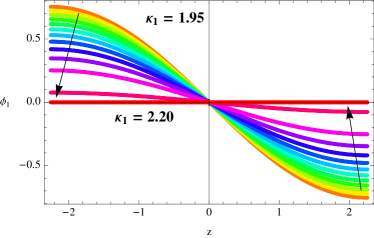
(a) $\phi^{\rm saddle}_{1}(z)$

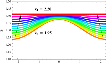
(b) $\phi^{\rm saddle}_{2}(z)$

Figure 1: The saddle states $\phi^{\rm saddle}_{i=1,2}$ passed by the system at different relative field stiffnesses ($=\kappa_{1}$). The evolution of the saddle is described as the continuous transition of colors. $\kappa_{1}$ was increased from 1.95 to 2.20 with an increment of 0.01. The arrows indicate the suppression of the instanton at $L>L_{c}(1)=\frac{\pi}{\sqrt{\mu 1-\mu 2}}$ as $\kappa_{1}$ increases. Here $\mu_{1}=3$, $\mu_{2}=2$, and $L=4.51$.

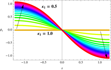
(a) $\phi^{\rm saddle}_{1}(z)$

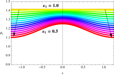
(b) $\phi^{\rm saddle}_{2}(z)$

Figure 2: The saddle states $\phi^{\rm saddle}_{i=1,2}$ passed by the system at different relative field stiffnesses(=$\kappa_{1}$). The evolution of the saddle is described as the continuous transition of colors. $\kappa_{1}$ was decreased from 1.0 to 0.5 with a decrement of -0.01. The arrows indicate the retrieval of the instanton at $L<L_{c}(1)=\frac{\pi}{\sqrt{\mu 1-\mu 2}}$ as $\kappa_{1}$ decreases. Here $\mu_{1}=3$, $\mu_{2}=2$, and $L=0.25$.

As noted earlier (cf. (8), $L_{c}(1)=\frac{\pi}{\sqrt{\mu_{1}-\mu_{2}}}$: below $L_{c}(1)$ the saddle is spatially uniform, and above $L_{c}(1)$ it is spatially varying [1]. The situation becomes more complicated when $\kappa_{1}\neq 1$. Fig. 1 summarizes our results when $\mu_{1}=3$, $\mu_{2}=2$ and $L>L_{c}(1)=\pi$. In this and Fig. 2, the saddle state (whether uniform or instanton) is denoted $\phi_{i}^{\rm saddle}(z),i=1,2$. We find that as $\kappa_{1}$ increases, the spatial variation of the instanton becomes increasingly suppressed until the instanton finally collapses to the uniform state. Conversely, when $L<L_{c}(1)$, the instanton state is retrieved for $\kappa_{1}<1$ (cf. Fig. 2).

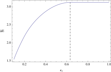
(a) $L=2.50$

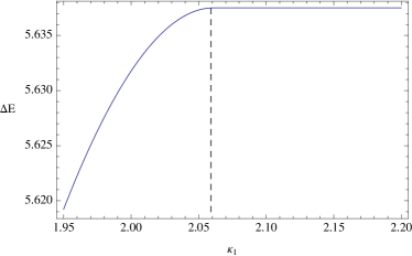
(b) $L=4.51$

Figure 3: Energy of the saddle state as a function of $\kappa_{1}$, where $\Delta E=E_{saddle}-E_{metastable}$. The dashed lines indicate that $\kappa_{1c}\approx 0.63$ for $L=2.50$ and $\kappa_{1c}\approx 2.06$ for $L=4.51$, where energies of the instanton and uniform saddles cross. The region $\kappa_{1}<\kappa_{1c}(L)$ corresponds to the instanton saddle, and $\kappa_{1}>\kappa_{1c}(L)$ to the uniform saddle. Here $\mu_{1}=3$, and $\mu_{2}=2$.

This effect can be understood as follows. In the limit of low noise, the transition occurs over the saddle state of least energy. An increase in $\kappa_{1}$ raises the bending energy of any nonuniform configuration, and therefore that of the instanton, while leaving the energy of the uniform saddle unchanged. When the energies of these two states cross, the activation process switches from one saddle state to the other. This is seen explicitly in Fig. 3, where we plot the energy of the saddle state against $\kappa_{1}$ for both $L=0.25$ and $L=4.51$. In these figures the curve to the left of the dashed line is the instanton branch, which increases monotonically until it reaches a constant value: the energy of the uniform saddle state.

We next investigated the question of whether the transition from uniform saddle to instanton (or vice-versa) as $\kappa_{1}$ varies occurs as a continuous crossover or as an abrupt phase transition. If the latter, then we also need to determine the order of the transition.

In [1], the uniform $\to$ instanton saddle transition was induced by changing $L$ at fixed $\kappa_{1}$. There we concluded that the transition was reminiscent of a second-order phase transition, in the asymptotic $\epsilon\to 0$ limit. This follows from the continuity of the activation energy at all values of $L$, including $L_{c}(1)$. (For examples of potentials where the activation energy jumps at a precise value of $L$, corresponding to a first-order transition, see [21].) In fact, it can be shown analytically that the first derivative of the activation energy curve with respect to $L$ is also continuous everywhere, but the second derivative is discontinuous at $L_{c}(1)$.

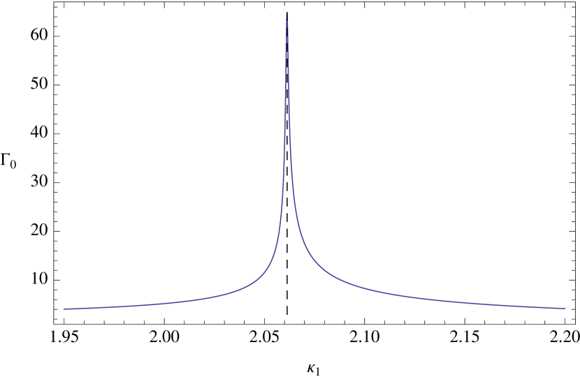
Figure 4: Behavior of the prefactor $\Gamma_{0}$ as calculated numerically using (10) when $\mu_{1}=3$, $\mu_{2}=2$, and $L=4.51$.

Similarly, Fig. 3 suggests that there is indeed a continuous phase transition, in that the activation energy changes continuously as one passes through the transition, as $\kappa_{1}$ varies for fixed $L$. This continuity leads to a divergence in the transition rate prefactor, shown in Fig. 4 (similar to that induced by changing $L$ at fixed $\kappa_{1}$ in [1]). The value of $\kappa_{1c}(L=4.51)$ where the prefactor diverges and that where the energies of the respective saddles cross agree to within a numerical error of $10^{-2}$.

What causes this divergence? Away from criticality, the spectrum of the linearized dynamical operator $\Lambda_{u}$ about the saddle consists of a single negative eigenvalue, whose corresponding eigenvector determines the unstable direction, with all other eigenvalues positive. As criticality is approached, the smallest positive eigenvalue, denoted $\lambda_{u,2}$, approaches zero. This signals the mathematical divergence on the “normal” lengthscale of $O(\epsilon^{1/2})$ of fluctuations about the saddle, and by (10) is seen to lead to divergence of the prefactor. (For a discussion of how to interpret this “divergence”, see [22].)

The eigenvalue spectrum about the uniform saddle can be analytically calculated [1]. The eigenvalue $\lambda_{u,2}$ is found to be

$$\lambda_{u,2}=\frac{\kappa_{1}\pi^{2}}{L^{2}}-(\mu_{1}-\mu_{2})\,.$$ (12)

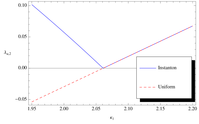
Figure 5: Smallest nonnegative eigenvalue $\lambda_{u,2}$ (solid line) of the saddle state for $\mu_{1}=3$, $\mu_{2}=2$ and $L=4.51$. For $\kappa_{1}<2.06$ this eigenvalue corresponds to the instanton saddle, and for $\kappa_{1}>2.06$ to the uniform saddle. The extended dashed line shows the continuation of this eigenvalue for the uniform saddle in its unstable regime below $\kappa_{1c}$.

At fixed $L$, this switches from negative (unstable) to positive (stable) as $\kappa_{1}$ increases, as shown in Fig. 5. This change of sign corresponds to a transition from an instanton saddle to a uniform one as $\kappa_{1}$ varies. Using this approach, the curve $L_{c}$ vs. $\kappa_{1c}$ can be derived analytically as the locus of points where $\lambda_{u,2}=0$ and thus the full phase diagram determined as represented by the solid curve in Fig. 6.

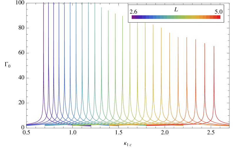
Figure 7: The divergence of $\Gamma_{0}$ at $L$ ranging from $2.6$ to $5.0$. Here $\mu_{1}=3$, $\mu_{2}=2$, and the values of $\kappa_{1c}$ (or the corresponding $L_{c}$) correspond to the dots in Fig. 6. The peaks are of different heights because the speeds of divergence are not necessarily the same for every $L$.

We have also studied the behavior of the transition rate prefactor in a wide range of values of $L$ numerically, all of which lead to the same conclusion as described above. Fig. 7 shows the divergence of $\Gamma_{0}$ at different $L_{c}$’s and their corresponding $\kappa_{1c}$’s.

5 Discussion

We have solved the general two-field model of (1) and (2) for its full parameter space. We have uncovered a new mechanism for the transition in the switching rate, and shown that it has features of a second-order phase transition.

In the one-field case, the mechanism behind the transition is not difficult to understand. At smaller $L$ (recall that this is a dimensionless lengthscale, in units of a reduced length that includes the single bending coefficient $\kappa$), bending costs (in conformity with the boundary condition) are prohibitive, and the uniform saddle therefore has lower energy than the instanton. At large lengthscales, the uniform saddle has a prohibitive bulk energy (i.e., potential difference with the stable state), whereas the instanton differs from one or the other stable state only within the domain wall region, whose lengthscale remains of $O(1)$. What is perhaps less intuitive is that the transition in saddle states should be asymptotically (as $\epsilon\to 0$) sharp.

Here we have uncovered a second mechanism for the transition to occur: as noted in Sec. 4, increase of $\kappa_{1}$ when $L>L_{c}(1)$ suppresses spatial variation, causing the instanton (again in a sharp transition) to collapse to the uniform saddle. Conversely, the instanton state can be retrieved for $L<L_{c}(1)$ when $\kappa_{1}$ decreases; of course, bending becomes increasingly favorable energetically. The result is a phase diagram in $(L,\kappa_{1}/\kappa_{2})$ space, as in Fig. 6, where a phase separation line denotes the boundary between the uniform and instanton “phases”.

We close with some remarks about the string method as applied to this problem.

A randomly placed string will relax towards the most probable transition path along the stable direction of the saddle. In Sec. 4 we defined the smallest positive eigenvalue (corresponding to the stable direction) of the linearized operator $\Lambda_{u}$. As a second-order phase transition is approached, $\lambda_{u,2}$ drops to $0^{+}$, so that the energy landscape curvature in the stable direction becomes very small. When the string arrives in its neighborhood, the restoring force exerted along its normal direction correspondingly becomes small leading to slow convergence. If one sits right at the critical point, the string will not arrive at the saddle.

The string method assumes that most of the probability flux from the reactant to the product state is carried by one (or more generally a few) paths through the saddle state, in each of which the probability flux is tightly confined to a narrow quasi - 1D region in state space. However, near criticality the path splays out in the direction normal to the longitudinal transition path. In this case one needs to consider transition “tubes”, inside which most of probability flux is concentrated. The equilibrium condition (11) corresponds to conditions away from criticality, where the transition tube is thin.

The equation for the path of maximum flux is derived in [23], where it is noted that the reaction flux intensity must be maximized along the thin transition tube (or the string, when using the string method). An alternative derivation can be found in [24].

Acknowledgments. The authors are grateful to Weiqing Ren and Ning Xuan for helpful discussions. We are especially grateful to Gabriel Chaves for his help in programming the string method. This work was supported in part by NSF Grant PHY-0965015.

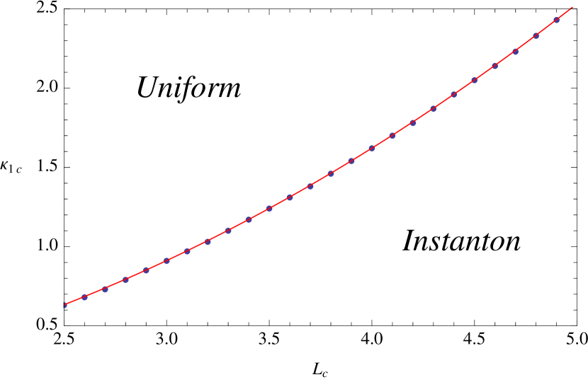
Figure 6: The phase diagram at $\mu_{1}=3$, $\mu_{2}=2$. The dots represent numerically determined values where the energies of the uniform and instanton saddles cross. The solid line was computed analytically using (12), that is, by determining the relation between $\kappa_{1}$ and $L$ along which the smallest nonnegative eigenvalue of the uniform saddle is zero.

References

- [1] L. Gong and D. L. Stein, “The escape problem in a classical field theory with two coupled fields,” J. Phys. A: Math. Theor., vol. 43, p. 405004, 2010.
- [2] K. Martens, D. L. Stein, and A. D. Kent, “Thermally induced magnetic switching in thin ferromagnetic annuli,” in Noise in Complex Systems and Stochastic Dynamics III (L. B. Kish, K. Lindenberg, and Z. Gingl, eds.), pp. 1–11, SPIE Proceedings Series, 2005.
- [3] K. Martens, D. L. Stein, and A. D. Kent, “Magnetic reversal in nanoscopic ferromagnetic rings,” Phys. Rev. B, vol. 73, p. 054413, 2006.
- [4] M. C. Cross and P. C. Hohenberg, “Pattern formation outside of equilibrium,” Rev. Mod. Phys., vol. 65, pp. 851–1112, 1993.
- [5] Y. Tu, “Worm structure in the modified Swift–Hohenberg equation for electroconvection,” Phys. Rev. E, vol. 56, pp. R3765–R3768, 1997.
- [6] U. Bisang and G. Ahlers, “Thermal fluctuations, subcritical bifurcation, and nucleation of localized states in electroconvection,” Phys. Rev. Lett., vol. 80, pp. 3061–3064, 1998.
- [7] A. M. Dikande, “Microscopic domain walls in quantum ferroelectrics,” Phys. Lett. A, vol. 220, pp. 335–341, 1996.
- [8] D. A. Gorokhov and G. Blatter, “Decay of metastable states: Sharp transition from quantum to classical behavior,” Phys. Rev. B, vol. 56, pp. 3130–3139, 1997.
- [9] J. Bürki, C. A. Stafford, and D. L. Stein, “Theory of metastability in simple metal nanowires,” Phys. Rev. Lett., vol. 95, pp. 090601–1–090601–4, 2005.
- [10] J. Bürki, C. A. Stafford, and D. L. Stein, “Comment on ‘Nonlinear current-voltage curves of gold quantum point contacts’,” Appl. Phys. Lett., vol. 88, p. 166101, 2006.
- [11] R. S. Maier and D. L. Stein, “Droplet nucleation and domain wall motion in a bounded interval,” Phys. Rev. Lett., vol. 87, pp. 270601–1–270601–4, 2001.
- [12] R. S. Maier and D. L. Stein, “Effects of weak spatiotemporal noise on a bistable one-dimensional system,” in Noise in Complex Systems and Stochastic Dynamics (L. Schimansky-Geier, D. Abbott, A. Neiman, and C. V. den Broeck, eds.), vol. 5114, pp. 67–78, SPIE Proceedings Series, 2003.
- [13] J. Bürki, C. A. Stafford, and D. L. Stein, “Fluctuational instabilities of alkali and noble metal nanowires,” in Noise in Complex Systems and Stochastic Dynamics II (Z. Gingl, J. M. Sancho, L. Schimansky-Geier, and J. Kertesz, eds.), pp. 367–379, SPIE Proceedings Series, 2004.
- [14] D. F. Urban, J. Bürki, C.-H. Zhang, C. A. Stafford, and H. Grabert, “Jahn-Teller distortions and the supershell effect in metal nanowires,” Phys. Rev. Lett., vol. 93, pp. 186403–1–186403–4, 2004.
- [15] M. Tarlie, E. Shimshoni, and P. Goldbart, “Intrinsic dissipative fluctuation rate in mesoscopic superconducting rings,” Phys. Rev. B, vol. 49, pp. 494–497, 1994.
- [16] J. Bürki, R. E. Goldstein, and C. A. Stafford, “Quantum necking in stressed metallic nanowires,” Phys. Rev. Lett., vol. 91, pp. 254501–1–254501–4, 2003.
- [17] M. Abramowitz and I. A. Stegun, eds., Handbook of Mathematical Functions. New York: Dover, 1965.
- [18] M. Yoshida, Y. Oshima, and K. Takayanagi, “Nonlinear current-voltage curves of gold quantum point contacts,” Appl. Phys. Lett., vol. 87, pp. 103104–1–103104–3, 2005.
- [19] W. E, W. Ren, and E. Vanden-Eijnden, “String method for the study of rare events,” Phys. Rev. B, vol. 66, p. 052301, 2002.
- [20] W. E, W. Ren, and E. Vanden-Eijnden, “Simplified and improved string method for computing the minimum energy paths in barrier-crossing events,” J. Chem. Phys., vol. 126, p. 164103, 2007.
- [21] J. Bürki, C. A. Stafford, and D. L. Stein, “The order of phase transitions in barrier crossing,” Phys. Rev. E, vol. 77, p. 061115, 2008.
- [22] D. L. Stein, “Critical behavior of the Kramers escape rate in asymmetric classical field theories,” J. Statist. Physics, vol. 114, pp. 1537–1556, 2004.
- [23] W. E and E. Vanden-Eijnden, “Transition-path theory and path-finding algorithms for the study of rare events,” Annual Review of Physical Chemistry, vol. 61, pp. 391–420, 2010.
- [24] M. J. Berkowitz M, Morgan JD and N. SH, “Diffusion-controlled reactions: a variational formula for the optimum reaction coordinate,” J. Chem. Phys., vol. 79, pp. 5563–65, 1983.