A GLOBAL TURBULENCE MODLE FOR NEUTRINO-DRIVEN CONVECTION IN CORE-COLLAPSE SUPERNOVAE

Abstract

Simulations of core-collapse supernovae (CCSNe) result in successful explosions once the neutrino luminosity exceeds a critical curve, and recent simulations indicate that turbulence further enables explosion by reducing this critical neutrino luminosity. We propose a theoretical framework to derive this result and take the first steps by deriving the governing mean-field equations. Using Reynolds decomposition, we decompose flow variables into background and turbulent flows and derive self-consistent averaged equations for their evolution. As basic requirements for the CCSN problem, these equations naturally incorporate steady-state accretion, neutrino heating and cooling, non-zero entropy gradients, and turbulence terms associated with buoyant driving, redistribution, and dissipation. Furthermore, analysis of two-dimensional (2D) CCSN simulations validate these Reynolds-averaged equations, and we show that the physics of turbulence entirely accounts for the differences between 1D and 2D CCSN simulations. As a prelude to deriving the reduction in the critical luminosity, we identify the turbulent terms that most influence the conditions for explosion. Generically, turbulence equations require closure models, but these closure models depend upon the macroscopic properties of the flow. To derive a closure model that is appropriate for CCSNe, we cull the literature for relevant closure models and compare each with 2D simulations. These models employ local closure approximations and fail to reproduce the global properties of neutrino-driven turbulence. Motivated by the generic failure of these local models, we propose an original model for turbulence which incorporates global properties of the flow. This global model accurately reproduces the turbulence profiles and evolution of 2D CCSN simulations.

1. Introduction

Though our understanding of the core-collapse supernova (CCSN) explosion mechanism remains incomplete, recent simulations indicate that it is likely to involve multi-dimensional effects. In fact, in all proposed mechanisms neutrino-driven convection plays an important, if not vital, role. Motivated by these results, we present a theoretical framework to investigate the role of turbulence in launching successful explosions. Furthermore, we lay down the foundation for this framework by deriving self-consistent steady-state equations for the background and turbulent flows.

The fundamental problem of CCSN theory is to determine how the stalled shock transitions into a dynamic explosion. Within a few milliseconds after bounce, the core-bounce shock wave stalls into an accretion shock (Mazurek, 1982; Bruenn, 1985, 1989). Unchecked, continued accretion through the shock would form a black hole (O’Connor & Ott, 2011). However, the preponderance of observed neutron stars (Lorimer et al., 2006) and supernova (SN) explosions (Li et al., 2010) dictates that the stalled shock is revived into an explosion most of the time.

For more than two decades, the favored mechanism for core collapse supernovae has been the delayed-neutrino mechanism (Bethe & Wilson, 1985). In this model, a neutrino luminosity of several times 10⁵² erg/s cools the protoneutron star and heats the region below the shock. Under the correct conditions, this heating by neutrinos can revive the shock and produce an explosion. Unfortunately, except for the least massive stars which undergo core collapse, most of the detailed 1D neutrino-transport-hydrodynamic simulations do not produce solutions containing explosions (Liebendörfer et al., 2001b, a; Rampp & Janka, 2002; Buras et al., 2003; Thompson et al., 2003; Liebendörfer et al., 2005; Kitaura et al., 2006).

While most 1D simulations fail to produce explosive solutions, recent 2D simulations show promising trends. These simulations capture multi-dimensional instabilities that aide the neutrino mechanism in driving explosions (Marek & Janka, 2007; Murphy & Burrows, 2008b; Scheck et al., 2008; Marek & Janka, 2009; Fernández & Thompson, 2009; Suwa et al., 2010; Nordhaus et al., 2010). These instabilities include neutrino-driven convection (Burrows et al., 1995; Janka & Müller, 1995; Murphy & Burrows, 2008b; Nordhaus et al., 2010) and the standing accretion shock instability (SASI) (Blondin et al., 2003; Ohnishi et al., 2006; Burrows et al., 2006; Marek & Janka, 2007, 2009; Foglizzo & Tagger, 2000; Foglizzo, 2009). Besides these two instabilities, other multi-dimensional processes may revive the stalled shock, including magnetohydrodynamic (MHD) jets (Burrows et al., 2007a; Dessart et al., 2008) and acoustic power derived from asymmetric accretion and an oscillating PNS (Burrows et al., 2006, 2007b). Though the prevalence of these last two processes is still debated (Dessart et al., 2008; Weinberg & Quataert, 2008), two points remain clear: (1) the solution to the CCSN problem is likely to depend on multi-dimensional effects, and (2) in all proposed mechanisms, neutrinos and turbulence play an important, if not central, role. Hence, whatever the mechanism, it is important to understand the role of neutrinos and turbulence.

Burrows & Goshy (1993) proposed that if a critical neutrino luminosity is exceeded for a given mass accretion rate, the neutrino mechanism succeeds. These authors developed a steady-state model for an accretion shock in the presence of a parametrized neutrino heating and cooling profile. The two most important parameters of the steady-state model are the neutrino luminosity $L_{\nu_{e}}$ and mass accretion rate $\dot{M}$. They found no steady-state solutions for luminosities above a critical curve $L_{\nu_{e},crit}=f(\dot{M})$, and interpreted this curve as separating steady-state (or failed supernova) solutions from explosive solutions. However, this work did not prove that the solutions above the critical curve are in fact explosive, nor did they consider multidimensional effects.

Using a similar neutrino parametrization as in the Burrows & Goshy (1993) work, Murphy & Burrows (2008b) showed in 1D and 2D simulations that the solutions above the critical luminosity are in fact explosive. Moreover, they found that the critical luminosity in the 2D simulations is $\sim$70% of that in 1D for a given $\dot{M}$. Additional investigations by Nordhaus et al. (2010) show that the critical luminosity is even further reduced in 3D. These results suggest that the critical luminosity is a useful theoretical framework for describing the conditions for successful explosions (Burrows & Goshy, 1993; Murphy & Burrows, 2008b).

Initial investigations by Murphy & Burrows (2008b) also suggest that the reduction in the critical luminosity is caused by turbulence. An alternative but related condition for explosion is a comparison of the advection and heating timescales (Thompson, 2000; Janka, 2001; Thompson et al., 2003; Murphy & Burrows, 2008b). The heating timescale is the time it takes to significantly heat a parcel of matter, and the advection timescale is the time to advect through this region. If the advection timescale is long compared to the heating timescale, then explosion ensues. In 1D, as matter accretes onto the PNS, it is limited to advect through the gain region with one short timescale. In 2D, convective motions increase the dwell time, which leads to more heating for the same neutrino luminosity and a lower critical luminosity(Murphy & Burrows, 2008b). Pejcha & Thompson (2011) have recently challenged this explanation and suggest that rather than increasing the heating, turbulence acts to reduce the cooling. Regardless, the simulations show that the critical luminosity is lower in the presence of convection.

These results suggest that a theory for successful explosions requires a theoretical framework for turbulence and its influence on the critical luminosity. In this paper, we develop the foundation for such a framework. Recent developments in turbulence theory have led to accurate turbulence models, and in this paper we use similar strategies to develop a turbulence model appropriate for CCSNe. Such a turbulence model can then be incorporated into steady-state accretion models to derive reduced critical luminosities for explosion, as well as used in 1D radiation-hydrodynamic (RHD) simulations to expedite systematic studies of core-collapse physics. In the present paper, we develop a turbulence model which captures the salient features of 2D core collapse convection, but eventually the model must be calibrated against 3D simulations.

To develop a turbulence model appropriate for core-collapse turbulence, we use a general and fully self-consistent approach called Reynolds decomposition (Plate et al., 1997; Pope, 2000; Launder & Sandham, 2002). The first step in this approach is to decompose the flow variables into averaged and fluctuating components. Evolution equations for the mean flow variables are then developed by writing the conservation laws in terms of these mean and fluctuating components and then averaging. The resulting evolution equations for the mean fields contain terms which involve both the mean fields as well as correlations of fluctuating components. These correlations represent the action of turbulence and include the Reynolds stress, turbulent kinetic energy, turbulent enthalpy flux, and higher order correlations. These evolution equations are self-consistent and naturally include the effects of a background flow, which is important in core collapse. Unfortunately, this procedure always produces evolution equations which depend on a correlation of higher order than the evolution equations. Therefore, in order to develop a closed system of equations, the highest order correlations must be modeled in terms of the lower order correlations and mean fields. Furthermore, closure depends upon the macroscopic flow itself, so there is no unique closure for turbulence. This is the infamous closure problem of turbulence.

Fortunately, there is a small class of turbulent flows (e.g., shear, buoyancy driven, etc.) and closure models have been developed that work well for each type under a range of conditions (Turner, 1973; Plate et al., 1997; Pope, 2000; Launder & Sandham, 2002; Wilcox, 2006). The general strategy to find closure relations involves an interplay between theory, observations, and numerical simulations (Launder & Sandham, 2002). First, terms in the mean-field equations are compared to either observations or numerical simulations. Approximations are then proposed for the higher order correlation terms that satisfy the observations/simulations and provide closure. This approach has been used successfully for geophysical flows (Launder & Sandham, 2002) and is now being applied to stellar structure calculations (Garaud et al., 2010; Meakin & Arnett, 2007).

Following on these successes, we use this strategy to develop a turbulence model for the core-collapse problem in which buoyancy and a background accretion flow dominate. In § 2, we use Reynolds decomposition to formally derive the averaged background and turbulence equations and identify terms that are important for neutrino-driven convection. Using 2D simulations, we examine in § 3 the turbulent properties of neutrino-driven convection and show that the turbulence equations which we derive in § 2 are consistent with the simulated flows. Finding solutions to the mean-field equations requires a closure model. Therefore, in § 4 we present several models representative of the literature. However, these fail to reproduce the global profiles of neutrino-driven convection, leading us to develop a novel global model. In §5, we compare the results of the turbulence models (§ 4) with the results of 2D simulations and conclude that our global model is the only model to reproduce the global properties of neutrino-driven convection. In § 6, using the mean-field equations and 2D simulations, we investigate the effects of turbulence on the conditions for successful explosions. Finally, in §7 we summarize our findings, and motivate the need for a similar analysis using 3D simulation data.

2. Background and Turbulence Equations: Reynolds Decomposition

The first step in understanding the effects of turbulence is to derive the governing steady-state equations. Therefore, in this section, we use Reynolds decomposition to derive exact equations for the steady-state background and turbulent flows.

Historically, turbulence modelers have used two approaches to derive the models. In one, ad hoc equations are suggested to model the important turbulence physics. These are often of practical use, but the underlying assumptions often make these of limited use. Mixing length theory (MLT) is one such approach (see §4.5 for its limitations) (Kippenhahn & Wiegert, 1990). In the second approach, one derives self-consistent equations for turbulence by decomposing the hydrodynamic equations into background and turbulent parts. Reynolds decomposition is an example of this approach. Though these equations are exact, they are not complete; they need a model for closure. If the ad hoc approaches accurately represent Nature, then one should be able to derive them by making the appropriate assumptions in the exact equations. Therefore, regardless of the technique employed, starting with the self-consistent equations enables a better understanding of the assumptions and limitations. In this paper, we pursue both approaches, but in this section, we use Reynolds decomposition to derive and explore the self-consistent equations for the background and turbulent flows.

In Reynolds decomposition, the hydrodynamic equations are decomposed into background and turbulent flows (Pope, 2000). Consider a generic flow variable, $\phi$, and its decomposition into average (background) and fluctuating (turbulent) components: $\phi=\phi_{0}+\phi^{\prime}$. The mean-field background of $\phi$, $\left<\phi\right>$, is obtained by coarse spatial and temporal averages. The interval for the averages must be large or long enough to smooth out short term turbulent fluctuations, but they must not be too large or long so that interesting spatial or temporal trends in the mean-field quantities are completely averaged out. Choosing the scales of the averaging window is dependent upon the problem, and in this paper, we define $\langle\rangle$ as averaging over the solid angle in the spherical coordinate system and over a fraction of the eddy crossing time of the convective region. By definition, the coarse average of $\phi$ is $\left<\phi\right>=\phi_{0}$ and the mean-field average of the fluctuation is identically zero, $\left<\phi^{\prime}\right>=0$. Therefore, first order moments of turbulent fluctuations are identically zero and only higher order terms survive. For example, the average of the velocity fluctuation is zero, $\left<\textbf{\em v}^{\prime}\right>$, but the mean-field of the second order term, the Reynolds stress $\left<\mathbf{R}\right>=\left<\textbf{\em v}^{\prime}\otimes\textbf{\em v}^{\prime}\right>$, is nonzero.

2.1. Averaged Background Equations

The general equations for mass, momentum, and entropy conservation are

$$\frac{\partial\rho}{\partial t}+\nabla\cdot\left(\rho\textbf{\em u}\right)=0\,,$$ (1)

$$\frac{\partial\left(\rho\textbf{\em u}\right)}{\partial t}+\nabla\cdot\left(\rho\textbf{\em u}\otimes\textbf{\em u}\right)=-\nabla P+\rho\textbf{\em g}\,,$$ (2)

and

$$T\left(\frac{\partial\left(\rho s\right)}{\partial t}+\nabla\cdot\left(\rho s\textbf{\em u}\right)\right)=\rho\dot{q}\,.$$ (3)

In these equations, the density, velocity, pressure, temperature, and specific entropy are $\rho$, u, $P$, $T$, and $s$. g is the gravitational acceleration, and $\dot{q}$ is the specific local heating and/or cooling rate.

After Reynolds decomposition, averaging, and assuming steady state, the hydrodynamics equations, eqs. (1-3), become

$$\nabla\cdot(\rho_{0}\textbf{\em v}+\left<\rho^{\prime}\textbf{\em v}^{\prime}\right>)=0\,,$$ (4)

$$\left<\rho\textbf{\em u}\right>\cdot\nabla\textbf{\em v}=-\nabla P_{0}+\rho_{0}\textbf{\em g}-\nabla\cdot\left<\rho\mathbf{R}\right>\,$$ (5)

and

$$\left<\rho\textbf{\em u}\right>\cdot\nabla s_{0}=\left<\frac{\rho\dot{q}}{T}\right>+\frac{\rho_{0}\epsilon}{T_{0}}-\nabla\cdot\left<\textbf{\em F}_{s}\right>\,.$$ (6)

For all quantities, the turbulent perturbations are denoted by a superscript ${\prime}$, and, with the exception of velocity, the background flow is denoted by subscript $0$. The background velocity is v, and the perturbed velocity is $\textbf{\em v}^{\prime}$.

Equations 4-6 are very similar to the usual steady-state equations of hydrodynamics, but the last term in all three equations add new turbulence physics. Conservation of mass flux is split between the background and the turbulence, $\left<\rho^{\prime}\textbf{\em v}^{\prime}\right>$. In the momentum equation, the extra force due to turbulence is the divergence of the Reynolds stress, $\mathbf{R}=\textbf{\em v}^{\prime}\otimes\textbf{\em v}^{\prime}$. The entropy equation has two new terms; the divergence of the entropy flux, $\textbf{\em F}_{s}=\rho s^{\prime}\textbf{\em v}^{\prime}$, represents entropy redistribution by turbulence, and $\epsilon$ represents heat due to turbulence dissipation. For isotropic turbulence, the divergence of $\mathbf{R}$ can be re-cast as the gradient of turbulent pressure: i.e. $-(2/3)\nabla(\rho K)$, where $K=\textbf{\em v}^{\prime}\cdot\textbf{\em v}^{\prime}/2$ is the turbulent kinetic energy. Using thermodynamic relations, we reduce the number of turbulent correlations in eqs. (4-6) by noting that $\left<\rho^{\prime}\textbf{\em v}^{\prime}\right>=\eta\textbf{\em F}_{s}$, where $\eta=\beta_{T}/c_{P}$, $c_{P}$ is the specific heat at constant pressure, and $\beta_{T}=-(\partial\ln\rho/\partial\ln T)_{P}$ is the logarithmic derivative of density with respect to temperature at constant pressure.

While we consider the convective entropy flux, $\textbf{\em F}_{s}$, traditionally, astrophysicists have considered the enthalpy flux, $\textbf{\em F}_{e}=\rho_{0}c_{P}\left<\textbf{\em v}^{\prime}T^{\prime}\right>$ in turbulence models. The enthalpy flux has units of energy flux. Therefore, the enthalpy flux is a natural choice for stellar structure calculations in which the enthalpy flux and radiative flux must add to give the total luminosity of the star. Because the convective region is semi-transparent to neutrinos, there is no such constraint in the core-collapse problem. Furthermore, since we decompose the entropy equation, the entropy flux is the most natural flux to consider. For the instances that require discussing the enthalpy flux, we express it in terms of the entropy flux, $\textbf{\em F}_{e}=T_{0}\textbf{\em F}_{s}$.

In expressing ($\langle\rho^{\prime}\textbf{\em v}^{\prime}\rangle=\eta\textbf{\em F}_{s}$, we have eliminated one of the turbulent correlations , but there still remain three turbulent correlations ($\mathbf{R}$, $\textbf{\em F}_{s}$, and $\epsilon$), resulting in more unknowns than equations. To close these equations, we derive the turbulence equations in § 2.2).

2.2. Averaged Equations for Turbulent Correlations

Using the definitions of $\mathbf{R}$ and $\textbf{\em F}_{s}$ and the conservation equations, we re-derive the evolution equations for the Reynolds stress ($\mathbf{R}$) and the entropy flux ($\textbf{\em F}_{s}$). For similar derivations of these equations, see Canuto (1993) and Garaud et al. (2010). The convective Reynolds stress equation is

$$\begin{array}[]{lllr}\lx@intercol\@ADDCLASS{ltx_eqn_lefteqn}$\displaystyle\partial\langle\rho\mathbf{R}\rangle/\partial t+\textbf{\em v}\cdot\nabla\left<\rho\mathbf{R}\right>+\left<\rho\mathbf{R}\right>\otimes\nabla\cdot\textbf{\em v}=$\mbox{}\hfil\lx@intercol\\ &&+\left<\rho^{\prime}\textbf{\em v}^{\prime}\right>\otimes\textbf{\em g}+[\left<\rho^{\prime}\textbf{\em v}^{\prime}\right>\otimes\textbf{\em g}]^{\mathsf{T}}&\textrm{Buoyant production}\\ &&-\left<\rho\mathbf{R}\right>\cdot\nabla\textbf{\em v}-[\left<\rho\mathbf{R}\right>\cdot\nabla\textbf{\em v}]^{\mathsf{T}}&\textrm{Shear production}\\ &&-\langle\nabla\otimes\textbf{\em F}_{P}+[\nabla\otimes\textbf{\em F}_{P}]^{\mathsf{T}}\rangle&\textrm{Pressure flux}\\ &&+\langle P^{\prime}\nabla\textbf{\em v}^{\prime}+[P^{\prime}\nabla\textbf{\em v}^{\prime}]^{\mathsf{T}}\rangle&\textrm{Pressure strain}\\ &&-\nabla\cdot\left<\rho\textbf{\em v}^{\prime}\otimes\mathbf{R}\right>&\textrm{Turbulent transport}\\ &&-\rho_{0}\boldsymbol{\varepsilon}&\textrm{Dissipation}\,,\\ \end{array}$$ (7)

where the turbulent pressure flux is $\textbf{\em F}_{P}=P^{\prime}\textbf{\em v}^{\prime}$, the dissipation tensor is $\rho_{0}\boldsymbol{\varepsilon}=\mu[\nabla^{2}\left<\mathbf{R}\right>-2(\nabla\textbf{\em v}^{\prime})\cdot(\nabla\textbf{\em v}^{\prime})]$, and $[]^{\mathsf{T}}$ is the transpose operator. In eq. (7), we separate the terms on the right-hand-side into rows to better illustrate their physical relevance. They are buoyant and shear production, redistribution by the turbulent pressure flux, the pressure-strain correlation, turbulent Reynolds stress transport, and the turbulent dissipation. In neutrino-driven convection of core collapse, buoyancy is the most important turbulent production. In terms of driving turbulence, the shear production term is less important. However, this term and the pressure-strain term are primarily responsible for redistributing stress among the components. For example, gravity acts mostly on the vertical stress components, but the shear production and pressure-strain terms redistribute stress to the horizontal components. Also important in redistributing stress is the turbulent transport term. In fact, in the next paragraph, we show that this term is in effect the divergence of the turbulent kinetic energy flux, which is very important in vertical kinetic energy transport.

Taking the trace of the Reynolds stress equation gives the convective kinetic energy equation:

$$\begin{array}[]{llll}\lx@intercol\@ADDCLASS{ltx_eqn_lefteqn}$\displaystyle\partial\langle\rho K\rangle/\partial t+\textbf{\em v}\cdot\nabla\left<\rho K\right>+\left<\rho K\right>\nabla\cdot\textbf{\em v}=$\mbox{}\hfil\lx@intercol\\ &&&+\left<\rho^{\prime}\textbf{\em v}^{\prime}\right>\cdot\textbf{\em g}-\mbox{tr}\left(\left<\rho\mathbf{R}\right>\cdot\nabla\textbf{\em v}\right)\\ &&&-\nabla\cdot\left<\textbf{\em F}_{K}\right>-\nabla\cdot\langle\textbf{\em F}_{P}\rangle+\left<P^{\prime}\nabla\cdot\textbf{\em v}^{\prime}\right>-\rho_{0}\epsilon\,,\\ \end{array}$$ (8)

where $\mbox{tr}()$ is the trace operator, the turbulent dissipation becomes $\epsilon=\mbox{tr}(\boldsymbol{\varepsilon})/2$, and $\textbf{\em F}_{K}=\rho\textbf{\em v}^{\prime}K$ is the turbulent kinetic energy flux. Once again on the right-hand-side, we have the familiar terms: buoyancy and shear production, turbulent redistribution by the turbulent kinetic energy flux, the divergence of the pressure flux, work done by turbulent pressure, and turbulent dissipation.

The corresponding equation for convective entropy flux is

$$\begin{array}[]{lllr}\lx@intercol\@ADDCLASS{ltx_eqn_lefteqn}$\displaystyle\partial\langle\textbf{\em F}_{s}\rangle/\partial t+\textbf{\em v}\cdot\nabla\left<\textbf{\em F}_{s}\right>+\left<\textbf{\em F}_{s}\right>\nabla\cdot\textbf{\em v}=$\mbox{}\hfil\lx@intercol\\ &&+\rho_{0}\eta\left<Q\right>\textbf{\em g}&\textrm{Buoyant production}\\ &&-\left<\textbf{\em F}_{s}\right>\cdot\nabla\textbf{\em v}-\left<\rho\mathbf{R}\cdot\right>\nabla s_{0}&\textrm{Gradient production}\\ &&-\left<s^{\prime}\nabla P^{\prime}\right>&\textrm{Pressure covariance}\\ &&-\nabla\cdot\left<\textbf{\em v}^{\prime}\otimes\textbf{\em F}_{s}\right>&\textrm{Turbulent transport}\\ &&+\left<\rho\textbf{\em v}^{\prime}\dot{q}/T\right>&\textrm{heat production}\,.\\ \end{array}$$ (9)

where $Q={s^{\prime}}^{2}$ is the variance of the entropy perturbation. Once again, we separate the terms in eq. (9) into rows to highlight their physical significance. The terms in the entropy flux equation are analogous to the terms in the Reynolds stress equation. They are buoyant and gradient production terms, the pressure-covariance, turbulent transport, and heat production. Unlike the Reynolds stress equation, we find that buoyant production, gradient production, pressure covariance, and turbulent transport are all equally relevant in determining the entropy flux.

The first term on the right hand side of eq. (9) is the buoyant production. This term is an important source in eq. (9), but it depends upon yet another correlation, the variance of the entropy perturbation. The corresponding equation for the entropy variance is

$$\begin{array}[]{lllr}\hbox to0.0pt{$\displaystyle\partial\langle\rho Q\rangle/\partial t+\nabla\cdot\left(\rho\textbf{\em v}\langle Q\rangle\right)=$\hss}\\ &&-2\left<\textbf{\em F}_{s}\right>\cdot\nabla s_{0}&\textrm{Gradient Production}\\ &&+2\langle s^{\prime}\dot{Q}/T\rangle&\textrm{Heat Production}\\ &&-\nabla\cdot\left<\rho\textbf{\em v}^{\prime}Q\right>&\textrm{Turbulent Transport}\,.\\ \end{array}$$ (10)

Equations (7-10) are an exact set of evolution equations for the 2^nd order correlations (i.e. Reynolds stress, entropy flux, and entropy variance). While these equations are exact, they are not complete. Each equation depends upon 3^rd order correlations, necessitating further evolution equations for the higher order correlations. However, it is impossible to close the turbulence equations in this way, as each set of evolution equations depends upon yet higher order correlations. The only solution is to develop a closure model to relate higher order moments to lower order moments.

This is analogous to the closure problem in deriving the hydrodynamics equations. In the hydrodynamics equations, the equation of state (EOS) is a microphysical closure model which relates the pressure (a higher moment) to the density and internal energy. Because of the vast separation of scale, the EOS depends upon microphysical processes only and is independent of the macroscopic hydrodynamical flows. Hence, as a closure model, the EOS enables the hydrodynamic equations to be relevant for a wide range of macroscopic flows. Conversely, turbulence occupies the full range of scales from the microscopic to the largest bulk flows. In some cases, turbulence is the dominant macroscopic flow. Consequently, closure is necessarily dependent upon the macroscopic flow, making it impossible to derive a generic closure relation for turbulence.

To find solutions to the turbulence equations, we need to construct a turbulence closure model that is appropriate for core collapse. The standard approach is to develop a turbulence closure model for each macroscopic flow. Fortunately, this task is not as daunting as it first appears. Turbulence can be divided into several classes that are characterized by the driving mechanism (i.e. shear, buoyancy, magnetic) and closure models have been constructed that are appropriate for each class. For core collapse, buoyancy is the primary driving force, and the rest of this paper is devoted to finding an appropriate buoyancy closure model for core-collapse turbulence.

2.3. Steady-state Reynolds-averaged Equations in Spherical Symmetry

Assuming a spherically symmetric background, the equations for the background flow (eqs. 4-6) become

$$\dot{M}=4\pi r^{2}\dot{m}=4\pi r^{2}(\rho_{0}v_{r}+\left<\rho^{\prime}v^{\prime}_{r}\right>)\,,$$ (11)

$$\dot{m}\,\partial_{r}v_{r}=-\partial_{r}P_{0}+\rho_{0}g_{r}-\partial_{r}\left<\rho R_{rr}\right>-\frac{2\left<\rho R_{rr}\right>}{r}+\frac{\left<\rho(R_{\theta\theta}+R_{\phi\phi})\right>}{r}\,,$$ (12)

and

$$\dot{m}\,\partial_{r}s_{0}=\left<\frac{\rho\dot{q}}{T}\right>+\frac{\rho_{0}\epsilon}{T_{0}}-\nabla_{r}\cdot\left<F_{r}\right>\,,$$ (13)

where the $r$, $\theta$, and $\phi$ subscripts refer to the radial and angular components in spherical coordinates. Therefore, $\partial_{r}$ is the partial derivative with respect to $r$, and $\nabla_{r}\cdot$ is the radial part of the divergence. Since we assume steady state, the mass accretion rate, $\dot{M}$, is a constant. For isotropic turbulence, the last three terms of eq. (12) reduce to $\partial_{r}\left<\frac{2}{3}\rho K\right>$, the gradient of turbulent pressure. However, Arnett et al. (2009) note that buoyancy-driven turbulence in spherical stars is not isotropic but is most consistent with $R_{rr}=R_{\theta\theta}+R_{\phi\phi}$ and $R_{\theta\theta}=R_{\phi\phi}$. In this work, we adopt this later assumption where convenient, but we retain the general expression in eq. (12) as a reminder that the relationships among the Reynolds stress components must be determined by theory, simulation, or experiment.

The equivalent steady-state and spherically symmetric equations for Reynolds stress, entropy flux, and entropy variation are

$$\begin{array}[]{lll}\lx@intercol\@ADDCLASS{ltx_eqn_lefteqn}$\displaystyle v_{r}\partial_{r}\left<\rho R_{rr}\right>+\left<\rho R_{rr}\right>\nabla_{r}\cdot v_{r}=$\mbox{}\hfil\lx@intercol\\ &&+2\left<\rho^{\prime}v^{\prime}_{r}\right>g_{r}-2\left<\rho R_{rr}\right>\partial_{r}v_{r}\\ &&-\left<v^{\prime}_{r}\partial_{r}P^{\prime}+\partial_{r}P^{\prime}v^{\prime}_{r}\right>-\nabla_{r}\cdot\left<\rho v_{r}^{\prime}R_{rr}\right>-\rho_{0}\varepsilon_{rr}\,,\\ \end{array}$$ (14)

$$v_{r}\partial_{r}\left<\rho R_{\theta\theta}\right>+\left<\rho R_{\theta\theta}\right>\nabla_{r}\cdot v_{r}=-\nabla_{r}\cdot\left<\rho v_{r}^{\prime}R_{\theta\theta}\right>-\rho_{0}\varepsilon_{\theta\theta}\,,$$ (15)

$$v_{r}\partial_{r}\left<\rho R_{\phi\phi}\right>+\left<\rho R_{\phi\phi}\right>\nabla_{r}\cdot v_{r}=-\nabla\cdot\left<\rho v_{r}^{\prime}R_{\phi\phi}\right>-\rho_{0}\varepsilon_{\phi\phi}$$ (16)

$$\begin{array}[]{lllr}\lx@intercol\@ADDCLASS{ltx_eqn_lefteqn}$\displaystyle v_{r}\partial_{r}\left<F_{r}\right>+\left<F_{r}\right>\nabla_{r}\cdot v_{r}=$\mbox{}\hfil\lx@intercol\\ &&+\rho_{0}\eta\left<Q\right>g_{r}\\ &&-\left<F_{r}\right>\partial_{r}v_{r}-\left<\rho R_{rr}\right>\partial_{r}s_{0}\\ &&-\left<s^{\prime}\partial_{r}P^{\prime}\right>\\ &&-\partial_{r}\left<F_{r}v_{r}^{\prime}\right>-2\left<F_{r}v_{r}^{\prime}\right>/r+\left<F_{\theta}v^{\prime}_{\theta}+F_{\phi}v^{\prime}_{\phi}\right>/r\\ &&+\left<\rho v_{r}^{\prime}\dot{q}/T\right>\,,\\ \end{array}$$ (17)

and

$$\begin{array}[]{lllr}\lx@intercol\@ADDCLASS{ltx_eqn_lefteqn}$\displaystyle\rho_{0}v_{r}\partial_{r}Q+\nabla_{r}\cdot\left(\rho_{0}v_{r}\right)=$\mbox{}\hfil\lx@intercol\\ &&-2\left<F_{r}\right>\partial_{r}s_{0}+2\rho_{0}\eta\left<Q\right>\dot{q}/T_{0}-\nabla_{r}\cdot\left<\rho v_{r}^{\prime}Q\right>\,.\\ \end{array}$$ (18)

Finally, the spherically symmetric kinetic energy equation is

$$\begin{array}[]{llll}\lx@intercol\@ADDCLASS{ltx_eqn_lefteqn}$\displaystyle v_{r}\partial_{r}\left<\rho K\right>+\left<\rho K\right>\nabla_{r}\cdot v_{r}=$\mbox{}\hfil\lx@intercol\\ &&&+\left<\rho^{\prime}v^{\prime}_{r}\right>g_{r}+\left<\rho R_{rr}\right>\partial_{r}v_{r}\\ &&&-\nabla_{r}\cdot\left<F_{K}\right>-\nabla_{r}\cdot\left<F_{P}\right>+\left<P^{\prime}\nabla\cdot{\textbf{\em v}^{\prime}}\right>-\rho_{0}\epsilon\,.\\ \end{array}$$ (19)

3. Characterizing Turbulence of 2D Core-Collapse Simulations and Validating Averaged Equations

Having derived the mean-field equations and identified the important turbulent correlations, we now characterize the background and turbulent profiles of 2D simulations. Most importantly, we validate that the Reynolds averaged equations are consistent with the 2D results. Section 3.1 briefly describes the 2D simulations, highlighting general qualities that are relevant for turbulence analysis such as the location and extent of turbulence and neutrino heating and cooling. Then in §3.2, we characterize the turbulent correlations in the 2D simulations. Finally, in §3.3, we validate the averaged equations.

3.1. 2D Simulations

The 2D results presented here were calculated using BETHE-hydro (Murphy & Burrows, 2008a) and are the same simulations that were used in Murphy et al. (2009) to develop a gravitational wave emission model via turbulent plumes. While Murphy et al. (2009) considered a large suite of simulations, for clarity, we focus on one simulation that simulated the collapse and explosion of a solar metallicity, 15 M_⊙ progenitor model (Woosley & Heger, 2007) and used a driving neutrino luminosity of $3.7\times 10^{52}$ erg s^-1. See Murphy & Burrows (2008a) for more details on the technique and Murphy et al. (2009) for the setup of this particular 2D simulation.

To demonstrate the evolution of turbulence, most figures of this paper highlight three phases after bounce. These three stages correspond to modest steady-state convection (404 ms), growing convection and SASI (518 ms), and strong convection and SASI (632 ms), and the entropy color maps in Fig. 1 provide visual context for the shock location, heating and cooling, and location and extent of the turbulence.

Our focus is on the most obvious turbulent region, which extends from $\sim$80 km to the shock ($\gtrsim$180 km). This postshock turbulence is driven by neutrino heating, and in Fig. 2, we show neutrino heating (red), cooling (blue), and net heating (heating minus cooling, black lines) profiles for 1D (dashed-lines) and 2D (solid-lines) simulations. These local heating and cooling rates are calculated using eqs. (4-5) of Murphy & Burrows (2008b) and a neutrino luminosity of $L_{\nu_{e}}=3.7\times 10^{52}$ erg s^-1. Below the gain radius, $\sim$100 km, cooling dominates heating, but above the gain radius, heating dominates cooling. This latter region is called the gain region and drives turbulent convection. After matter accretes through the shock, it advects downward through the gain region, producing a negative entropy gradient. In turn, this negative entropy gradient drives buoyant convection. Though the region below the gain radius has a positive entropy gradient and is formally stable to convection, momentum carries plumes well into the cooling region (Murphy et al., 2009). This is a well known phenomenon in stellar convection and is called overshoot. In neutrino-driven convection, the depth of overshoot can be quite large, $\sim$20-40 km, (Murphy et al., 2009).

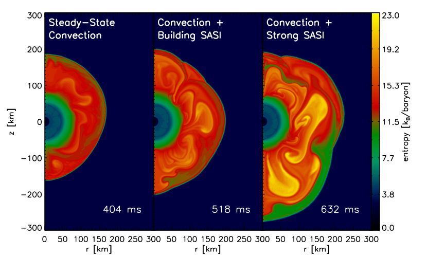
Figure 1.— Color map of entropy at times representing the three dominant phases. The left panel shows the flow during steady-state convection (404 ms after bounce), the middle panel illustrates the dynamics and entropy distribution during the building convection and SASI stage (518 ms), and the far right panel shows the flow during strong convection and SASI (632 ms). Most of the subsequent figures show specific turbulence characteristics at these three times.

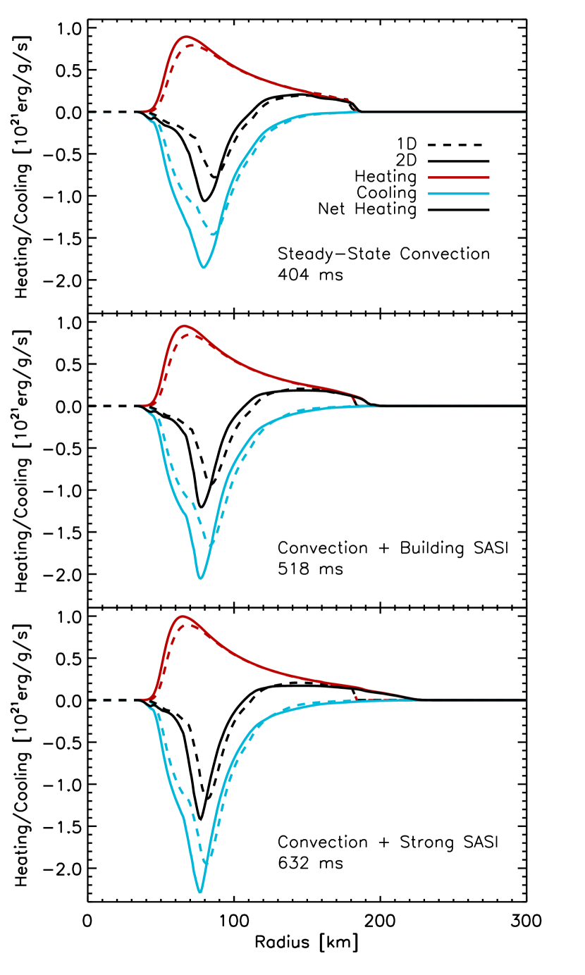
Figure 2.— Neutrino heating (red), cooling (blue), and net heating (black) profiles as a function of radius. The times correspond to the stages of post-bounce evolution highlighted in Fig. 1. This plot compares the 1D (dashed lines) and 2D (solid lines) profiles. Above the gain radius ($\sim$ 100 km), the net heating is positive. In this gain region, a negative entropy gradient formally drives buoyant convection. Below the gain region, a positive entropy gradient stabilizes against convection. Though only the gain region is formally convective, overshoot carries convection well into the stable region below (up to $\sim$40 km below). By definition, the heating profiles are similar. The cooling profiles show some minor differences, but these lead to minor differences in the entropy profiles (see Fig. 6). In Fig. 6, we show that the most notable differences between 1D and 2D are produced by the divergence of the convective entropy flux.

3.2. Turbulent Correlations of 2D Simulations

Figures 3 and 4 show the radial profiles of the primary correlations in the averaged equations, eqs. (4-10). The lowest moment correlations are the turbulent enthalpy flux ($T_{0}F_{s}$), the turbulent kinetic energies ($K_{r}$ & $K_{\theta}$; or Reynolds stresses), and the entropy variance ($Q$), and all three are shown in the top, middle, and bottom panels of Fig. 3. Other important higher order correlations are the turbulent transport terms, which are the transport of entropy flux, $\left<v^{\prime}_{r}F_{s}\right>$, the turbulent kinetic energy flux, $\left<F_{K}\right>$, and the entropy variance flux, $\left<\rho v^{\prime}_{r}Q\right>$. The radial profiles of these higher order correlations are in Fig. 4. In general, all turbulent correlations increase over time, and the radial profiles indicate that turbulence is dominated by coherent rising and sinking large-scale buoyant plumes.

The enthalpy (or entropy) flux has two broad physical interpretations. Most obviously, the entropy flux indicates the direction and magnitude of entropy transport due to turbulent motions. Naturally, positive and negative entropy fluxes correspond to upward and downward entropy transport. In addition to indicating the direction of entropy transport, the sign of the flux also indicates the direction of the buoyancy forces driving the turbulence. To understand this second interpretation, consider that the entropy flux is defined using the correlation of the velocity and entropy perturbations (i.e. $\left<s^{\prime}\textbf{\em v}^{\prime}\right>$). In regions where convection is actively driven, high entropy plumes rise buoyantly and low entropy plumes sink. In other words, the entropy and velocity perturbations are either both positive or negative. Hence, the correlation and entropy flux are always positive in regions of actively driven convection. At boundaries, where the plumes are decelerated due to a stable background, the correlation or entropy flux, is always negative. For example, as a low entropy plume penetrates into the lower stable layer, the sinking plume becomes immersed in a background that has even lower entropy. While the velocity perturbation remains negative, the entropy perturbation changes sign, becoming positive. Consequently, the correlation and entropy flux are negative in the bounding stabilizing regions.

With these interpretations of the entropy (enthalpy) flux, the top panel of Fig. 3 shows where convection is actively driven, where plumes are decelerated by bounding stable regions, and the magnitude of each as a function of time. At the shock, the entropy flux is zero. This is in contrast with the results of Yamasaki & Yamada (2006), who find an appreciable enthalpy flux at the shock. Whether the enthalpy flux is zero at the shock has consequences for the stalled-accretion shock solution (See § 4.3 for further discussion).

Naively, one would expect the gain radius ($\sim$100 km) to mark the boundary between actively driven convection in the heating region and the stabilizing effects in the cooling layers below. Though this is roughly correct, careful inspection of the enthalpy profiles show that the transition from positive to negative entropy flux does not correspond exactly with the gain radius. Instead, the gain radius corresponds best with the change in slope of the enthalpy profile. Above the gain radius, where convection is actively driven, the enthalpy profile has a negative gradient, and below the gain radius the gradient is positive.

This profile can be best understood considering a single low entropy plume originating at the shock. First of all, as this plume accelerates downward, both the entropy and velocity perturbations grow in magnitude. This explains the negative entropy flux gradient above the gain radius. Below the gain radius the background entropy gradient is positive. Therefore, the entropy perturbation diminishes as the background entropy reduces to the level of the low entropy plume. At this point, both the entropy perturbation and entropy flux are zero. Consequently, enthalpy flux gradient is positive below the gain radius. With a negative gradient above the gain region and a positive gradient below it, the enthalpy flux is maximum at the gain radius. As the plume’s inertia carries it beyond this radius, the enthalpy flux becomes negative in the stabilizing layers. These general characteristics are observed at all times, but with increasing magnitude at later times when convection is more vigorous.

The same simple model can explain the radial ($\left<K_{r}\right>$, green lines) and tangential ($\left<K_{\theta}\right>$, orange lines) kinetic energy profiles in the middle panel of Fig. 3. In fact, like the enthalpy flux, $\left<K_{r}\right>$ peaks at the gain radius. Because the sinking plumes have higher speeds than the rising plumes and the kinetic energy is weighted by the square of the speed, $\left<K_{r}\right>$ is dominated by the sinking plumes. Again, the radial profile of $\left<\right>$ is consistent with low entropy plumes originating at the shock, accelerating downward to a maximum speed at the gain radius, and decelerating in the stabilizing region below the gain radius. This is also consistent with the results of Murphy et al. (2009). The tangential component, $\left<K_{\theta}\right>$, on the other hand, shows a maximum just 10s of km away from the shock. This is where the rising plumes encounter material that has just passed through the shock and both turn their trajectories in the $\theta$-direction.

Interpretation of the entropy variance ($Q$ and the bottom panel of Fig. 3) is less clear. Like the enthalpy flux and kinetic energies, $Q$ increases with time. The most naive interpretation is that the variation of total heating among the sinking and rising plumes increases over time. However, it is not obvious whether this increase in variance is due to more heating or less cooling in either the rising or sinking plumes…or both. While it seems clear that the profiles of $T_{0}F_{s}$ and $K_{r}$ are dominated by the sinking plumes, there is circumstantial evidence that $Q$ might be dominated by the behavior of rising plumes. For one, there is a gradual rise in $Q$ from the lower convective boundary to the upper boundary, suggesting growth with the rise of buoyant plumes. But the most telling evidence comes from the entropy color maps of Fig. 1. In these maps, it is obvious that the entropy of the sinking plumes is roughly constant over time, while the entropy of rising plumes increases with time. Hence, the variance of entropy increases with time because the maximum entropy of the rising plumes increases.

All three transport terms in Fig. 4, $\left<v^{\prime}_{r}F_{s}\right>$, $\left<F_{K}\right>$, and $\left<\rho v^{\prime}_{r}Q\right>$, are negative nearly everywhere. Hence, the flow of core-collapse turbulence acts to transport entropy flux, kinetic energy, and entropy variance downward. This is typical of buoyancy driven convection and is observed in most simulations of convection within stellar interiors (Cattaneo et al., 1991; Meakin & Arnett, 2010). For the entropy flux, and turbulent kinetic energy, this fact further supports the notion that the turbulent correlations are dominated by sinking plumes. On the other hand, at first glance, the negative transport of $Q$ seems to be at odds with our previous conclusion that rising plumes dominate the character of $Q$. However, the moment of the entropy variance, $\left<Q\right>$, weights only the variance in the entropy, but the entropy variance flux weights the velocity of the plumes as well. In general, the speed of the sinking plumes is larger than the speed of rising plumes. Consequently, while rising plumes provide the most weight to $\left<Q\right>$, sinking plumes provide the greatest weight to $\left<\rho v^{\prime}_{r}Q\right>$. In §5, we present simple models for these transport terms that assume the dominance of sinking plumes.

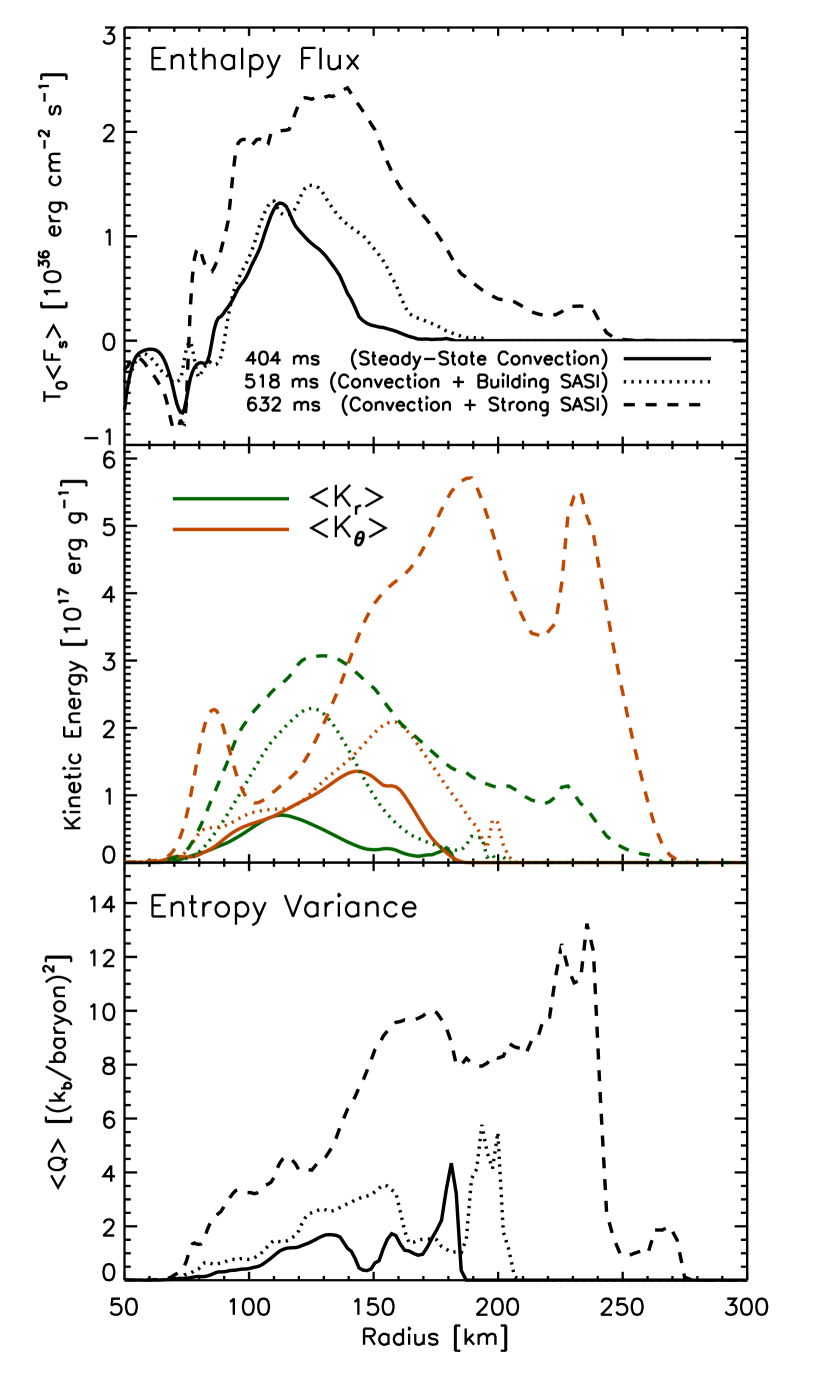
Figure 3.— Radial profiles for the most fundamental turbulent correlations: enthalpy flux, $T_{0}\left<F_{s}\right>$, (top panel), kinetic energies, $K_{r}$ & $K_{\theta}$, (middle panel), and entropy variance, , (bottom panel). The times correspond to the three postbounce phases shown in Fig. 1. These plots show that turbulence grows with time, and the radial profiles indicate that turbulence is dominated by non-local evolution of coherent large-scale buoyant plumes (see text for more details). A simple model that considers the evolution of sinking low entropy plumes explains the features of $T_{0}\left<F_{s}\right>$ and $\left<K_{r}\right>$ and rising high entropy plumes explain $\left<Q\right>$. See §3.2 for an explanation.

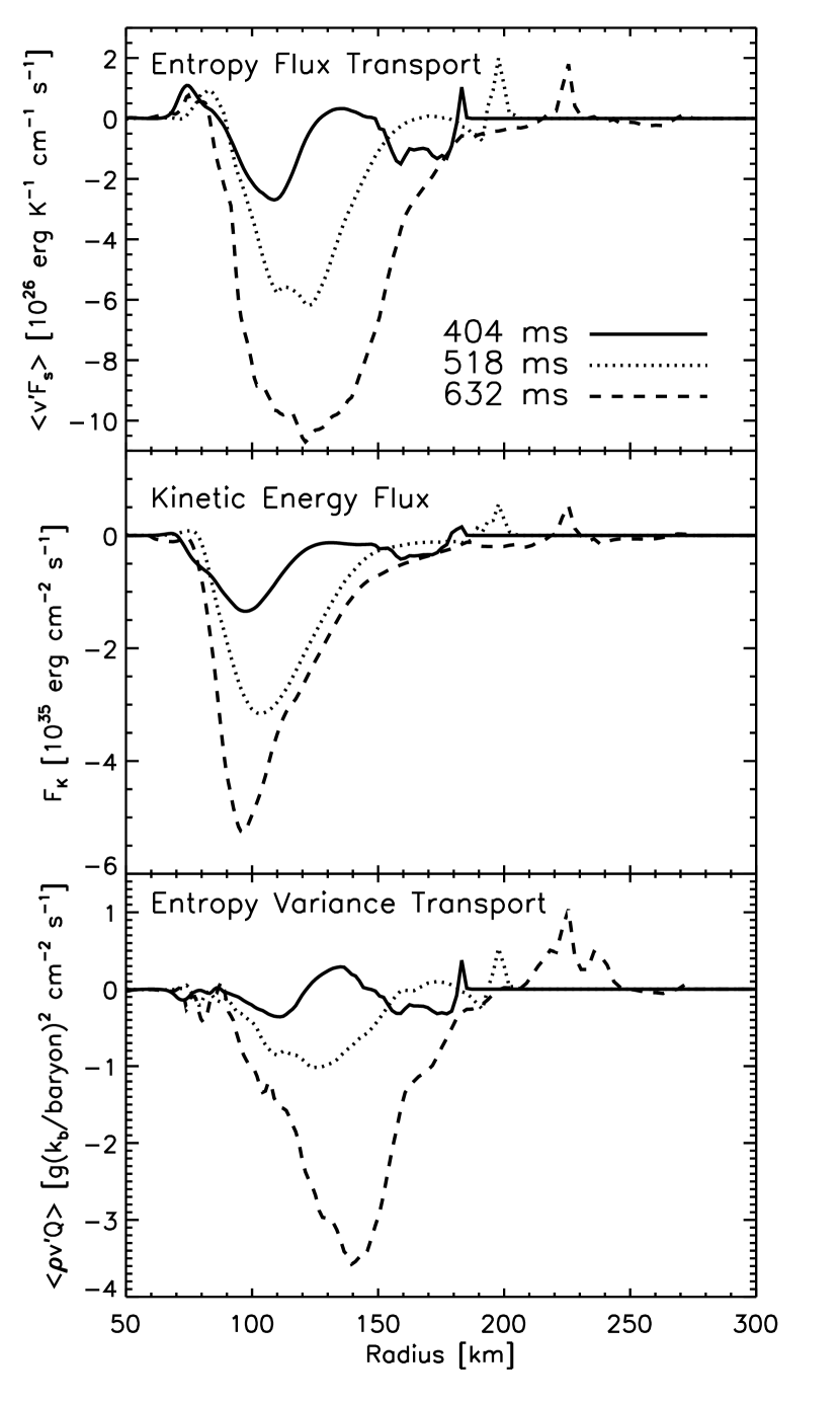
Figure 4.— Similar to Fig. 3 but for the transport of entropy flux, $\left<v^{\prime}F_{s}\right>$ (top panel), turbulent kinetic energy flux, $\left<F_{K}\right>$, and the entropy variance flux, $\left<\rho v^{\prime}Q\right>$. All transport terms are negative indicating that the transport of each correlation is dominated by the large speeds of the sinking plumes.

3.3. Comparing Averaged Background Equations with 2D Simulations

Having presented the turbulent correlations of 2D core-collapse simulations, we now validate the Reynolds-averaged equations. Specifically, we validate the spherically symmetric background equations, eqs. (11-13). For the sake of brevity, we do not show a plot of mass conservation but simply report that $\dot{M}=4\pi r^{2}(\rho_{0}v_{r}+\langle\rho^{\prime}v^{\prime}_{r}\rangle)$ is indeed satisfied in the 2D simulations.

Figure 5 validates the form of the momentum equation, eq. (12), including the turbulence terms. In the top panel, we plot the velocity profile of 1D and 2D simulations as a function of radius, and in the bottom panel, we plot the dominant force terms in the momentum equation for the 2D simulations only. Specifically, the bottom panel shows the difference in the gravitational and pressure gradient forces, $\rho_{0}\textbf{\em g}-\nabla P_{0}$ (dashed-line), and the divergence of the Reynolds stress, $\nabla\cdot\mathbf{R}$ (dotted line). The solid black line shows $\dot{m}\nabla_{r}v_{r}$ from the 2D simulation. This last term is the left-hand side of eq. (12), and in steady state, represents the total force per unit area that a Lagrangian parcel of matter experiences. If eq. (12) represents the correct derivation of the momentum equation including turbulence terms, then the sum of the right-hand side terms (dot-dashed red line) should equal the solid black line. Away from the shock, they agree quite well. Interestingly, the right-hand side is essentially zero in the heating region where convection is actively driven. This implies that the difference in the gravitational force and the pressure gradient is nearly balanced by the divergence of the Reynolds stress.

Figure 6 validates the Reynolds-averaged entropy equation, eq. (13). The solid black line corresponds to the 2D results, and the black dashed line shows the results of 1D simulations. For comparison, the red curve is the integration of eq. (13) using the 1D density, velocity, and heating profiles. Since the 1D simulations are not able to simulate multi-dimensional effects, we omit the turbulent dissipation and the entropy flux terms in this integration. The remarkable agreement between the results of this integration and the 1D simulation bolsters our approach in validating eq. (13). Similarly, the solid green line shows the integration of eq. (13) using the 2D density, velocity, and heating curves and no convection terms. This curve is similar to the 1D results and clearly under predicts the entropy in the gain region. On the other hand, including the turbulence terms in the integration of eq. (13) (dot-dashed green curve) dramatically improves the comparison. Therefore, given the right entropy flux and turbulent dissipation, we conclude that eq. (13) accurately determines the background flow. Additionally, we conclude that the turbulence models of §4 must, at a minimum, produce accurate entropy flux profiles to accurately describe the effects of convection in 2D simulations.

Figures 3-6 suggest that convection grows monotonically, but these figures sparsely sample convection and its effects at three times. In Fig. 7, we illustrate that convection indeed grows monotonically from core bounce until explosion. To provide some context with shock position, we plot in the top panel shock radii as a function of time after bounce. We show the 1D and average 2D shock radii using dashed and solid black lines, respectively. Before the onset of vigorous SASI and convection ($\sim$550 ms), both stall at $\sim$180 km. Afterward, the 2D average shock radius climbs to $\sim$320 km, at which point all measures of the shock unambiguously expand in an explosion. To illustrate the asymmetries in the shock we also plot the shock radius at the poles ($\theta$=0 and $\theta$ = $\pi$). The shock radii at the poles oscillate about the average shock position until explosion ($\sim$700 ms). The middle panel shows the maximum of the total, radial, and transverse kinetic energies. In general, the turbulent kinetic energy steadily grows until explosion. Finally, the bottom panel shows the maximum of 1D (black) and 2D (green) average entropy profiles. For comparison, we plot the maximum enthalpy flux in orange and the maximum entropy resulting from integrating eq. (13) in green. As in Fig. 6, the 2D simulation consistently shows higher entropy at all times, and the results of integrating eq. (13) are consistent with the simulations.

In conclusion, the results of Figs. (3-7) indicate that Reynolds decomposition of the hydrodynamics equations, eqs. (4-6), is consistent with 2D simulations.

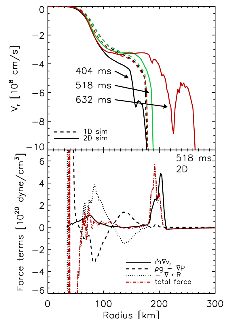
Figure 5.— Radial velocity (top panel) and force (bottom panel) profiles for the three phases shown in Fig. 1. The forces are the terms in the momentum equation, eq. (12) TOP PANEL: The 1D velocity profiles for the three phases are quite similar. The 2D velocity profiles evolve as the shock radius and convective vigor increase. At later times when convection is strongest, the velocity gradient tends to zero in the convective region. BOTTOM PANEL: We compare the individual force terms of the momentum equation, eq. (12). The excess force between gravity and the pressure gradient (dashed) is nearly balanced by the divergence of the Reynolds stress (dotted). The red dashed line shows that the sum of these forces do indeed equal the actual force, $\dot{m}\nabla v_{r}$ (solid curve). This validates the form of the momentum equation, eq. (12), including the convective term.

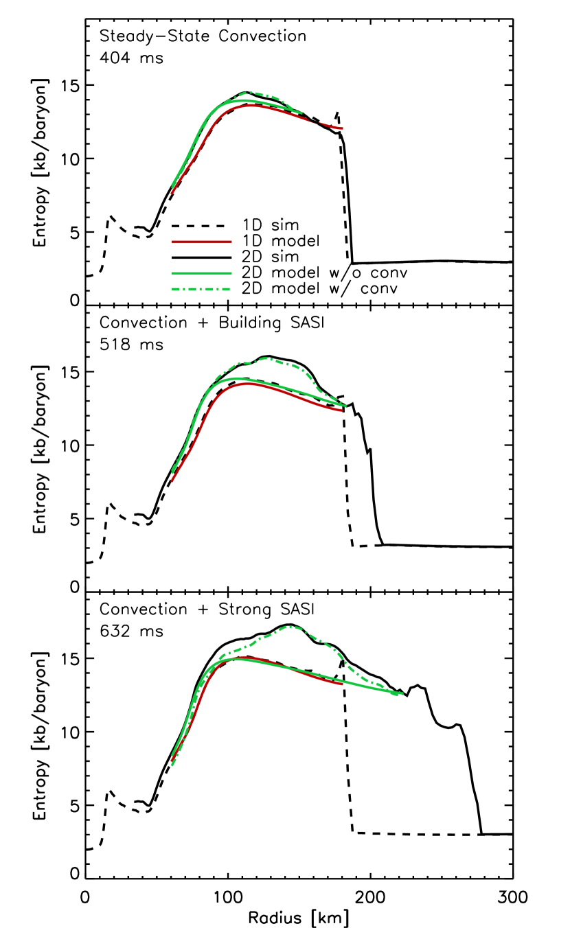
Figure 6.— Radial entropy profiles during the three phases shown in Fig 1. In these plots, we compare the results from 1D (dashed, black curves) and 2D (solid, black curves) simulations to integrations of the entropy equation, eq. (13). The red curve shows the result of this integration using background profiles from the 1D simulation and no convective terms. The agreement with 1D simulations validates this technique to verify the equations. The green curves show the results of integrating the entropy equation using background profiles from the 2D simulations without convective terms (solid green) and with convective terms (dashed green) curve. Excluding the convective terms under-predicts the entropy profile, and including the convective terms raises the entropy and produces accurate entropy profiles.

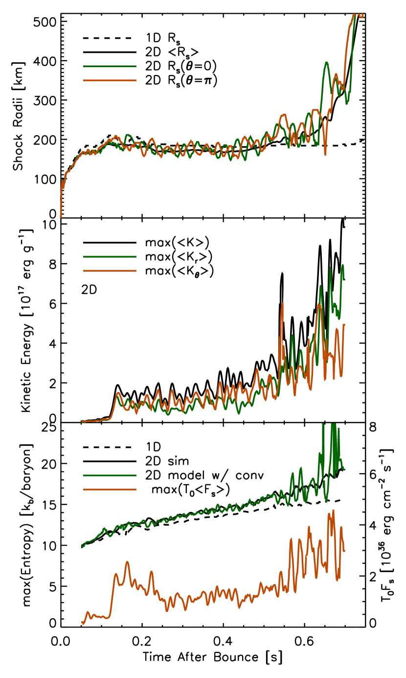
Figure 7.— A comparison of shock radii and convection diagnostics as a function of time after bounce. TOP PANEL: We plot shock radii as a function of time after bounce. We show the 1D and average 2D shock radii using dashed and solid black lines, respectively. Before the onset of vigorous SASI and convection ($\sim$550 ms), both stall at $\sim$180 km. Afterward, the 2D average shock radius begins to climb to $\sim$320 km, at which point all measures of shock radii expand outward in an explosion. To illustrate the asymmetries in the shock we also plot the shock radius at the poles ($\theta$=0 and $\theta$ = $\pi$). The shock radii at the poles oscillate about the average shock position until explosion ($\sim$700 ms). MIDDLE PANEL: The middle panel plots the maximum of the total, radial, and transverse kinetic energies. BOTTOM PANEL: The bottom panel shows the maximum entropy of the 1D and 2D simulations, the maximum entropy resulting from integrating eq. (13), and the maximum enthalpy flux $T_{0}\left<F_{s}\right>$. Figure 3 samples these convection diagnostics at three times and indicates that convection grows monotonically. These plots confirm that convection indeed grows with time. Furthermore, Fig. 6 validates the Reynolds-averaged entropy equation, eq. (13), at three specific times, and the bottom panel validates this equation at all times.

4. Turbulence Models

In § 2, we derived the turbulence equations, eqs. (4-10) and showed that they suffer from a closure problem. Therefore, finding solutions to the background and turbulence equations requires a turbulence closure model. In this section, we present several turbulence models and identify their strengths and weaknesses.

In sections 4.3-4.6, we present four turbulence models. These models, with the exception of Model 1, require a model for turbulent dissipation and transport. Therefore, our discussion of the models begins in sections 4.1 & 4.2 with a model for turbulence dissipation and transport. The next four sections, §4.3-4.5, present models for the primary 2^nd order turbulent correlations, $F_{s}$, $K$, and $Q$. The first model, Model 1, is a reproduction of a model presented by Yamasaki & Yamada (2006) and assumes that both $\left<\dot{s}\right>$ and $\nabla s_{0}$ are zero. The resulting model is simple, but it provides no equation for the turbulent kinetic energy. Model 2 is a closure model for the Reynolds stress, entropy flux, and entropy variance and has been designed and calibrated to simulate isolated buoyant plumes. Model 3 is an algebraic model which is akin to MLT.

To model the higher order correlations, Models 2 & 3 use expressions involving the local values of 2^nd-order correlations. Hence, some of the most important terms in a nonlocal problem are modeled using local approximations. While these local models are adequate in some locations, they can be factors off in other locations. Rather than relying on these local models, we develop in Model 4 (§ 4.6) a novel global model that uses global conservation laws to constrain the scale of convection.

Later, in § 5, we compare the results of these models to the turbulent kinetic energies and entropy flux of the 2D simulations.

4.1. Turbulent Dissipation: Kolmogorov’s Hypothesis

Starting with Kolmogorov’s hypotheses for turbulent dissipation, Arnett et al. (2009) construct a model for turbulent dissipation which they validate with 2D and 3D stellar evolution calculations. Buoyed by these successes, we construct a similar model for turbulent dissipation. One of the primary hypotheses of Kolmogorov’s theory is that turbulent energy is injected at the largest scales and cascades to smaller scales. Consequently, the rate of turbulent energy dissipation is governed by the largest scales and dimensionally is proportional to ${v^{\prime}}^{3}/\mathcal{L}$, where $\mathcal{L}$ is an appropriate length scale, usually the largest eddy size. Therefore, our model for turbulent dissipation is

$$\epsilon=\frac{R^{3/2}}{\mathcal{L}}\,,$$ (20)

where $R=\mbox{tr}(\mathbf{R})$ is the trace of the Reynolds stress tensor.

In most astrophysical calculations, the length scale is assumed to be proportional to the pressure scale height, $H_{P}=-(\partial\ln P/\partial r)^{-1}$. On the other hand, Arnett et al. (2009) found that stellar convection fills the total available space and that this also corresponds to the largest eddy size. For very large convection zones, they found that $\mathcal{L}$ is at most $4H_{P}$. Therefore, we set the length scale as $\mathcal{L}=\mbox{max}(4H_{P},\mathcal{L}_{\mbox{conv}})$, where $\mathcal{L}_{\mbox{conv}}$ is the size of the region unstable to convection.

Given Kolmogorov’s hypothesis, this model for $\epsilon$ is the most basic model that one can assume. Later in § 4.6, we propose a model for $\epsilon$ that satisfies Kolmogorov’s hypothesis but apparently represents the dissipation of buoyant plumes via entrainment. To satisfy global and local constraints for convection, we find that $\epsilon$ is best modeled by a linear function of distance from the shock. In 3D simulations of stellar convection in which negatively buoyant plumes dominate, Meakin & Arnett (2010) found a similar result. These results suggest that entrainment between rising and sinking plumes govern dissipation.

4.2. Turbulent Flux Models

The gradient diffusion approximation has found wide spread usage for closing the turbulent transport terms (e.g., Pope, 2000; Launder & Sandham, 2002). For example, Model 2, which we introduce in §4.4, uses this assumption. The theoretical basis for this closure model is two fold: first, the transported quantity behaves like a scalar; second, scale separation is a good approximation in the sense that transport is mediated by fluctuations on scales small compared to the largest scales characterizing the turbulent flow (Daly & Harlow, 1970). The turbulent transport in a buoyant convection zone, however, is generally recognized to be mediated by large scale coherent plumes (e.g. Cattaneo et al., 1991, and §3.2), thus challenging the theoretical underpinning for a gradient diffusion approximation. Furthermore, the shortcomings of the gradient diffusion approximation for thermal convection were explicitly illustrated through a series of 3D simulations of turbulent stellar interiors by Meakin & Arnett (2010).

Rather than a gradient diffusion approximation, we propose flux models that are proportional to ${R_{rr}}^{1/2}E_{i}$, where $E_{i}$ is the density of the transported quantity. This model is built on the advective nature of the transport in which $F_{i}\propto v^{\prime}E_{i}$. We propose the following models for turbulent transport of the entropy flux, turbulent kinetic energy, and entropy variance

$$\left<v^{\prime}_{r}F_{s}\right>\approx-R_{rr}^{1/2}F_{s},$$ (21)

$$\left<F_{K}\right>\approx-\rho_{0}R_{rr}^{3/2},$$ (22)

and

$$\left<\rho v^{\prime}_{r}Q\right>\approx-\frac{1}{2}\rho_{0}R_{rr}^{1/2}Q.$$ (23)

Except for the entropy variance flux, the comparison with 2D simulations (§5 and Fig. 9) indicates that the constant of proportionality is $\sim$1. The constant of proportionality for the entropy variance flux is found to be $\sim$1/2.

4.3. Model 1: Steady-State and Zero Entropy Gradient Model

The first turbulence model that we consider is a simple model for $F_{s}$ presented by Yamasaki & Yamada (2006). Yamasaki & Yamada (2006) assumed steady state and that the entropy gradient in eq. (13) is zero. From these assumptions, they derived a simple differential equation for the enthalpy flux. Here, we reproduce this equation, expressing it in terms of the entropy flux:

$$\nabla_{r}\cdot F_{s}=\frac{\dot{Q}}{T_{0}}\,.$$ (24)

A simple integral of this equation with a boundary condition leads to an expression for the entropy flux. Yamasaki & Yamada (2006) assumed zero flux at the lower boundary and integrated upward resulting in a nonzero flux at the shock.

A major advantage of this model is that it is simple and straightforward to find a solution for $F_{s}$. Unfortunately, the assumptions which lead to simplicity also lead to inaccurate turbulent profiles (see § 5). For one, there is no solution for the kinetic energies. Secondly, this model completely ignores the velocity of the background flow. As we show in § 5 and Fig. 12, this is inconsistent with the characteristics of neutrino-driven convection in 2D simulations. Thirdly, this model produces flawed entropy flux profiles. For example, it results in a nonzero entropy flux at the shock, while 2D simulations show zero entropy flux at the shock (Figure 3). In fact, the entropy flux is zero at both boundaries. To compensate for this nonzero flux at the shock, Yamasaki & Yamada (2006) modified the shock jump conditions. However, the solutions to eqs. 4-10 are quite sensitive to the form of the boundary conditions at the shock. Incorrect boundary conditions will lead to erroneous solutions.

4.4. Model 2: Reynolds Stress and Heat Flux Closure Model

Model 2 is a Reynolds stress and heat flux closure model that has been designed and calibrated to model isolated buoyant plumes (Launder & Sandham, 2002). Though core-collapse turbulence involves more than just isolated plumes, neutrino-driven convection is in fact buoyancy-driven. Therefore, it is plausible that the Reynolds stress and heat flux model might be an appropriate closure model.

The model for the Reynolds stress equation, eq. (7), is

$$\nabla\cdot(\rho\textbf{\em v}\otimes\mathbf{R})=\rho(\mathbf{G}+\mathbf{P}+\boldsymbol{\Pi}+\mathbf{D}-\frac{2}{3}\delta_{ij}\epsilon)\,,$$ (25)

where $\mathbf{G}$ and $\mathbf{P}$ are the buoyant and shear production terms, $\boldsymbol{\Pi}$ is the pressure-strain term, $\mathbf{D}$ is the diffusion term, and the final term is turbulent dissipation. All but the first two terms require models, and the expressions for the first two production terms are easily read from eq. (7).

The first of the modeled terms is the pressure-strain correlation, and it acts to redistribute energy among the Reynolds stress components. For buoyant flows, the pressure-strain correlation is generally modeled by three contributions

$$\boldsymbol{\Pi}=\boldsymbol{\Pi}_{1}+\boldsymbol{\Pi}_{2}+\boldsymbol{\Pi}_{3}\,,$$ (26)

where the first term is proportional turbulent stress, the second term is proportional to the interaction between turbulent stress and the mean strain, and the last term is proportional to buoyancy. Explicitly, they are

$$\boldsymbol{\Pi}_{1}=-c_{1}\frac{\epsilon}{K}\left(\mathbf{R}-\frac{2}{3}\delta_{ij}\rho K\right)\,,$$ (27)

$$\boldsymbol{\Pi}_{2}=-c_{2}\left(\mathbf{P}-\frac{1}{3}\delta_{ij}\mbox{tr}(\mathbf{P})\right)\,,$$ (28)

and

$$\boldsymbol{\Pi}_{3}=-c_{3}\left(\mathbf{G}-\frac{1}{3}\delta_{ij}\mbox{tr}(\mathbf{G})\right)\,,$$ (29)

where the parameters $c_{1}$, $c_{2}$, and $c_{3}$ are 3, 0.3, and 0.3 respectively.

Launder & Sandham (2002) suggest using the gradient-diffusion hypothesis to model the diffusion term. Specifically,

$$\mathbf{D}=c_{R}\nabla\cdot\left(\frac{K}{\epsilon}\mathbf{R}\cdot\nabla\mathbf{R}\right)\,,$$ (30)

where the constant $c_{R}$ has been calibrated by experiments and simulations to be 0.22. This diffusion term inherently assumes that the Reynolds stress (or kinetic energy) flux is proportional to the gradient in the Reynolds stress. This is most likely relevant in shear dominated flows. However, the buoyancy dominated flows of core-collapse convection are characterized by large scale plumes. As a consequence, the transport of kinetic energy flux is directly proportional to these bulk turbulent motions (i.e. $R^{3/2}$) rather than the gradient.

The final term to be modeled is the turbulent dissipation, $\epsilon$. Launder & Sandham (2002) add another differential equation that includes more production, diffusion, dissipation terms, and constants to be calibrated. To avoid these complications, we simply adopt the turbulence model of § 4.1.

To derive the model turbulent kinetic energy equation, we take the trace of the Reynolds stress model equation, eq. (25),

$$\begin{array}[]{llll}\lx@intercol\@ADDCLASS{ltx_eqn_lefteqn}$\displaystyle\textbf{\em v}\cdot\nabla\left<\rho K\right>+\left<\rho K\right>\nabla\cdot\textbf{\em v}=$\mbox{}\hfil\lx@intercol\\ &&&+\left<\rho^{\prime}\textbf{\em v}^{\prime}\right>\cdot\textbf{\em g}-\mbox{tr}\left(\left<\rho\mathbf{R}\right>\cdot\nabla\textbf{\em v}\right)\\ &&&c_{R}\nabla\cdot\left(\rho\frac{K}{\epsilon}\mathbf{R}\cdot\nabla K\right)-\rho_{0}\epsilon\,,\\ \end{array}$$ (31)

Except for two differences, this model kinetic energy equation is very similar to the full kinetic energy equation, eq. (8). The first difference is that the work done by turbulent pressure perturbations, $\left<P^{\prime}\nabla\cdot\textbf{\em v}^{\prime}\right>$, is absent in the model equation. Because the pressure-strain correlation, $\boldsymbol{\Pi}$, is designed to only redistribute energy among the components, the trace of this term is identically zero. Hence, the model assumes that this term is zero. Because low Mach number turbulence typically has negligible pressure perturbations, this is a standard assumption in turbulence modeling. Our 2D simulations confirm this assumption. The second difference is that $F_{K}$ is assumed to be proportional to $\nabla K$. This is a consequence of the gradient-diffusion approximation, but in § 5, we find that $F_{K}$ is not proportional to the gradient but is best modeled as $F_{K}\propto R^{3/2}$.

The model for the entropy flux equation, eq. (9), is

$$\begin{array}[]{llll}\lx@intercol\@ADDCLASS{ltx_eqn_lefteqn}$\displaystyle\textbf{\em v}\cdot\nabla\textbf{\em F}_{s}+\textbf{\em F}_{s}(\nabla\cdot\textbf{\em v})=$\mbox{}\hfil\lx@intercol\\ &&&\rho_{0}\eta Q\textbf{\em g}-\textbf{\em F}_{s}\cdot\nabla\textbf{\em v}-\mathbf{R}\cdot\nabla s_{0}\\ &&&+c_{s}\nabla\cdot\left(\frac{K}{\epsilon}\mathbf{R}\cdot\nabla\textbf{\em F}_{s}\right)+\boldsymbol{\Pi}_{s}\\ \end{array}$$ (32)

where $c_{s}=0.15$ and the pressure-entropy correlation term ($\boldsymbol{\Pi}_{s}$) is the analog of the pressure-strain correlation and is modeled by three terms

$$\boldsymbol{\Pi}_{s}=\boldsymbol{\Pi}_{s1}+\boldsymbol{\Pi}_{s2}+\boldsymbol{\Pi}_{s3}\,.$$ (33)

In general, these terms act to dissipate $\textbf{\em F}_{s}$ and represent pure turbulence, turbulence and mean strain, and buoyancy interactions:

$$\boldsymbol{\Pi}_{s1}=-c_{1s}\frac{\epsilon}{k}\textbf{\em F}_{s}\,,$$ (34)

$$\boldsymbol{\Pi}_{s2}=c_{2s}\textbf{\em F}_{s}\cdot\nabla\textbf{\em v}\,,$$ (35)

and

$$\boldsymbol{\Pi}_{s3}=c_{3s}\rho_{0}\eta Q\textbf{\em g}\,,$$ (36)

where the constants are $\{c_{1}s,c_{2}s,c_{3}s\}=\{2.85,0.55,0.55\}$. Once again, the transport term in eq. (32) is modeled using the gradient-diffusion approximation.

The final equation models the equation for entropy variance, eq. (10):

$$\rho\textbf{\em v}\cdot\nabla Q+Q\nabla\cdot(\rho\textbf{\em v})=-2\textbf{\em F}_{s}\cdot\nabla s_{0}c_{Q}\nabla\cdot\left(\rho\frac{K}{\epsilon}\mathbf{R}\cdot\nabla Q\right)-\frac{Q\rho\epsilon}{Kr}$$ (37)

where $c_{Q}=0.11$ and $r=0.56$.

Equations (25-37) represent a model for the turbulence equations that is complete and has been extensively tested and calibrated with experiment and simulations (Launder & Sandham, 2002). Unfortunately, there are several disadvantages to using this turbulence model. For one, this model depends upon a large number of calibrated constants. In addition, these equations were designed and calibrated to calculate the profile of a single isolated buoyant plume. The macroscopic flow of fully developed convection is very different. Therefore, it is quite possible that the closure relations presented in this model are not appropriate for core-collapse convection. Furthermore, the dissipation terms make eqs. (25-37) a stiff numerical problem, requiring careful numerical treatment. Consequently, the solutions to these equations are extremely sensitive to the uncertain dissipation models.

4.5. Model 3: An Algebraic Model

In general, there are two strategies to finding turbulent solutions (In § 4.6, we present a third). In the first, the turbulent correlations are solutions of differential equations. Models 1 & 2 are of this type. Within the second strategy, a few key assumptions allow the differential equations to be converted into a set of algebraic equations, and the turbulence correlations are solutions to these algebraic equations. An example of a turbulence model which uses a set of algebraic equations is the mixing length theory (MLT); it is used extensively through out astrophysics, including stellar structure calculations (Kippenhahn & Wiegert, 1990).

To transform the differential equations into algebraic equations, the temporal and spatial derivatives must either vanish or be approximated by algebraic expressions. As an example of the first method, one can assume that the temporal and advective derivatives are zero, (the L. H. S. of the evolution equations eqs. (7-10)). This assumption is valid in most circumstances because even though the terms on R.H.S. are large they often sum to zero. Therefore, the primary assumptions of this approach are steady state and local balancing. In the second approach, the spatial derivatives are replaced with ratios of the variable to be differentiated and a length scale. For example, the divergence of the kinetic energy flux is roughly, $\nabla\cdot F_{K}\sim F_{K}/L$. In effect, a global boundary value problem is reduced to a set of local algebraic expressions.

In some respects, these algebraic equations still retain nonlocal characteristics. The nonlocality is merely hidden in the assumptions. For example, in MLT, local gradients are used to calculate the local buoyancy force, but the eddies are assumed to remain coherent until a mixing length at which point they dissipate their energy. Hence, the finite size of the mixing length is an echo of the true nonlocality of turbulence in a local prescription. Where local balancing is important, such as the heating region, these approximations can give reasonable solutions. However, in regions where nonlocal transport is important, such as overshoot regions, these algebraic models fail completely.

To derive an algebraic model, we assume that transport balances buoyant driving. Applying this assumption to the exact 2^nd moment equations, eqs. (8-10), and using the flux models, eqs. (21-23), of §4.2 results in approximate kinetic energy,

$$-\nabla_{r}\cdot\left(\rho_{0}R^{3/2}_{rr}\right)\sim\eta F_{s}g\,,$$ (38)

entropy flux

$$-\nabla_{r}\cdot\left(R^{1/2}_{rr}F_{s}\right)\sim\frac{1}{2}\rho_{0}\eta gQ\,,$$ (39)

and entropy variance equations,

$$\nabla_{r}\cdot\left(\rho_{0}R^{1/2}_{rr}Q\right)\sim 4F_{s}\nabla s_{0}\,.$$ (40)

The R.H.S. of the approximate entropy flux equation, eq. (39), is a sum of two important terms: buoyancy driving, $\rho_{0}\eta gQ$, and the pressure covariance, $-\langle s^{\prime}\nabla P^{\prime}\rangle$. Launder & Sandham (2002) suggest that this term is best modeled by $-\langle s^{\prime}\nabla P^{\prime}\rangle\sim-(1/2)\rho_{0}\eta gQ$, and our 2D simulations confirm this model. In effect, the sum of these two source terms reduces buoyancy driving by a factor of two.

If we approximate the divergence of a generic flux, $F_{i}$, by $\nabla_{r}\cdot F_{i}\propto-F_{i}/z$, where $z=R_{s}-r$ is the downward distance from the shock, then algebraic solutions of the approximate equations are proportional to $z^{2}$. To obtain the correct proportionality constants, we assume solutions of the form $R_{rr}=az^{2}$, $F_{s}=bz^{2}$, and $Q=cz^{2}$, and substitute these into eqs. (38-40). This results in the following algebraic expressions for the second moment correlations

$$R_{rr}=\frac{2}{9}\eta g(-\partial_{r}s_{0})z^{2}\,,$$ (41)

$$F_{s}=\frac{8^{1/2}}{9}\rho_{0}\left(\eta g\right)^{1/2}\left(-\partial_{r}s_{0}\right)^{3/2}z^{2}\,,$$ (42)

and

$$Q=\frac{8}{9}\left(-\partial_{r}s_{0}z\right)^{2}\,.$$ (43)

For the entropy gradient in these equations, we assume that $\partial_{r}s_{0}\approx\dot{Q}/(\dot{m}T_{0})$, and to get the radial component of Reynolds stress we assume $R_{rr}\approx R/3$

If instead of assuming a balance between local driving and transport, we assume a balance between local driving and dissipation, then we obtain dimensionally similar results. However, they differ in the constants of proportionality and the length scale involved. With dissipation, the natural length scale is $\mathcal{L}$, which is a fixed scale and is either the full size of the convective region (i.e. a constant) or is proportional to the local scale height. In either case, using a fixed length scale results in algebraic expressions that are inconsistent with our 2D simulations. Instead, in §5, we show that the convective profiles in the driving region of 2D simulations are quite consistent with $z$ as the length scale. Interestingly, most contemporary formulations of MLT use $\mathcal{L}$ as the appropriate length scale, while in the original formulation of the MLT, Prandtl used $z$. In essence, the result that the downward distance, $z$, is the most appropriate length scale suggests that the properties of neutrino-driven convection are best modeled by negatively buoyant plumes that form at the shock and grow due to buoyancy.

4.6. Model 4: A General Global Turbulence Model

While the previous models are adequate in some locations, we show in § 5 that they fail to reproduce the global properties of neutrino-driven turbulence. Motivated by this failure, we propose an original turbulence model which is derived using global considerations.

Models 2 & 3 employ single-point closure models, which assume that on small scales, the higher order correlations can be modeled using local 2^nd-order correlations. Consequently, some of the most important terms in a nonlocal problem are modeled using local approximations. While these local models are adequate in some locations, they can be factors off in other locations. Given the stiff nature of the governing equations, these modest errors can lead to significantly flawed turbulent profiles. Rather than relying on these local models, we use conservation laws and develop an original global turbulence model.

Integrating the turbulence equations leads to global conservation laws for turbulence. For example, integrating the turbulent kinetic energy equation dictates that global buoyant driving equals global dissipation. To satisfy these global constraints, the turbulent correlations relax into the appropriate profiles. If the same driving, redistribution, and dissipation mechanisms operate in a wide range of conditions, then these global constraints also imply self-similar convection profiles. For Model 4, we adopt characteristic profiles for the convective entropy luminosity and turbulent dissipation. The specific profiles are motivated by the evolution of large scale buoyant plumes and informed by numerical 2D CCSN simulations (this paper) and 3D stellar convection (Meakin & Arnett, 2010). Then the scales of these profiles are constrained using the conservation laws. Given these scaled profiles, we then calculate the remaining quantities of interest such as the kinetic energy flux and entropy profile. The latter is particularly important in exploring the conditions for successful CCSN explosions.

Our global model builds upon and generalizes the ideas put forth by Meakin & Arnett (2010). In the context of stellar evolution and no background flow, Meakin & Arnett (2010) suggest that the primary role of the entropy (enthalpy) flux is to redistribute the entropy such that the entropy gradient is flat and the entropy generation rate is constant throughout. In other words, they found universal profiles for the entropy generation rate and entropy profiles. They then integrated the entropy and turbulent kinetic energy equations to provide integral constraints and solutions for the turbulent scales.

Similarly, the rate of entropy change in the CCSN context is uniform, in fact during the steady-state phase it is zero everywhere. However, the entropy gradient is nonzero, so the Meakin & Arnett (2010) model will not suffice. 2D simulations (see § 5) indicate that the global constraints and redistribution drive the convective entropy luminosity, $L_{s}=F_{s}4\pi r^{2}$, and turbulent dissipation to simple self-similar profiles.

Informed by 2D simulations of CCSNe (§ 5, Fig. 13) and 3D simulations of stellar convection (Meakin & Arnett, 2010), we model the convective entropy luminosity with a piecewise linear function,

$$L_{s}=\left\{\begin{array}[]{lr}L_{s,0}z/z_{0}\,,&{\rm for}\,z<z_{0}\\ L_{s,0}(Z_{c}-z)/(Z_{c}-z_{0})\,,&{\rm for}\,z>z_{0}\end{array}\right.\,,$$ (44)

and the turbulent dissipation via

$$\rho\epsilon 4\pi r^{2}\sim\alpha(R_{s}-r)\,,$$ (45)

where $z=r-R_{\ell}$ is the distance from the bottom of the convective region, $Z_{c}=R_{s}-R_{\ell}$ is the total size of the convective region, and $R_{\ell}$ is defined by $\int^{R_{S}}_{R_{\ell}}\dot{Q}/T_{0}\,dV=0$. In these models, the peak of the $L_{s}$ profile is at $z_{0}$, and goes to zero at $R_{\ell}$ and the shock. The turbulent dissipation is zero at the shock, and increases linearly downward with a scale of $\alpha$. Given the many differences (i.e dimensionality, accretion, etc.) between 2D CCSN and 3D stellar convection simulations, the universality of the profiles is remarkable and is a testament to their self-similarity. Taken together, this model for $L_{s}$ and $\epsilon$ has three parameters, $L_{s,0}$, $z_{0}$, and $\alpha$, which set the scale for convection.

Next, we use the algebraic expression for the entropy flux and global conservation laws to evaluate these scales. Operating under the assumption that the growth of negatively buoyant plumes sets the scale $L_{s,0}$, we evaluate the algebraic expression for the entropy flux, eq. (42), at the peak:

$$L_{s,0}=4\pi r^{2}F_{s,\textrm{alg}}(z_{0})\,.$$ (46)

We explore two techniques to constrain the position of the peak, $z_{0}$. In the first, we assume that the peak of $L_{s}$ corresponds to where entrainment starts to dominate the evolution of negatively buoyant plumes and that this distance is proportional to the pressure scale height (i.e. $Z_{c}-z_{0}=\alpha_{z_{0}}H_{p}$). Comparing to the 2D simulation, we find that $\alpha_{z_{0}}\simeq 1.7$, 2.1, and 2.0 at 404 ms, 518 ms, and 632 ms after bounce. Empirically, $\alpha_{z_{0}}\sim 2$ with an accuracy of $\sim$10%. While this empirical approach provides a useful diagnostic of $z_{0}$, it lacks a physical derivation.

In the second technique, we derive a physically motivated global constraint for $z_{0}$. Consider the approximate entropy flux and entropy variance equations, eqs. (39 & 40). They represent a set of conservation laws for $F_{s}$ and $Q$ in which the source terms are determined by buoyant driving. Combining these two equations and integrating over the whole convective region, we find that $\int F_{s}\cdot\nabla s_{0}dr\sim 0$. In effect, $F_{s}\cdot\nabla s_{0}$ represents an important buoyant source term for turbulence, where $F_{s}\cdot\nabla s_{0}$ is negative for the growth (decay) of negatively (positively) buoyant plumes and vice versa. Because $F_{s}=0$ and $Q=0$ at both boundaries, the integral of this buoyant source term must balance out. Therefore, we adjust $z_{0}$ so that $F_{s}$ satisfies

$$\int^{R_{s}}_{R_{\ell}}F_{s}\cdot\nabla s_{0}dr=0\,.$$ (47)

To set $\alpha$, the turbulent dissipation scale, we first rewrite the turbulent kinetic energy equation as an expression for the turbulent flux:

$$\frac{\partial L_{k}}{\partial r}=\eta L_{s}g_{r}-\rho\epsilon 4\pi r^{2}\,,$$ (48)

where we have neglected the term due to background advection. Integrating eq. (48) over the entire convective region and noting that $L_{K}$ is zero at the boundaries leads to the second conservation law for the balance of total buoyant work and dissipation:

$$\int^{R_{s}}_{R_{\ell}}\eta L_{s}g_{r}\,dr=\int^{R_{s}}_{R_{\ell}}\rho\epsilon 4\pi r^{2}\,dr\,.$$ (49)

Together, eqs. (46, 47, & 49) constrain the three scales of our global model.

Having set the scales of the turbulent profiles, eqs. (44) & (45), it is now possible to integrate eq. (48) to find the turbulent kinetic flux and, most importantly, evaluate the entropy profile including the effects of turbulence.

Including the time rate of change, the entropy equation is

$$\frac{\partial(\rho s_{0})}{\partial t}+\dot{m}\cdot\nabla s_{0}=\frac{\dot{Q}+\rho\epsilon}{T_{0}}-\nabla\cdot F_{s}\,,$$ (50)

and integrating this equation over the volume from an arbitrary radius, $r$ up to the shock, $R_{s}$ gives

$$\frac{\partial}{\partial t}\left(\int^{R_{s}}_{r}\rho s_{0}\,dV\right)+\dot{M}\Delta s_{0}(r)=L_{s}(r)+\int^{R_{s}}_{r}\frac{\dot{Q}}{T_{0}}\,dV+\int^{R_{s}}_{r}\frac{\rho\epsilon}{T_{0}}\,dV\,,$$ (51)

where $\Delta s_{0}(r)=s_{0}(R_{s})-s_{0}(r)$ and $L_{s}(r)=4\pi r^{2}F_{s}(r)$. Assuming a flat gradient, $\Delta s_{0}$ = 0, and $\partial s_{0}/\partial t=\langle(\dot{q}+\epsilon)/T_{0}\rangle_{m}$, where $\langle\rangle_{m}$ is a mass average, leads to the integral equation that Meakin & Arnett (2010) use for stellar convection. For the CCSN problem, we assume steady state, $\partial s_{0}/\partial t=0$ and $\Delta s_{0}\neq 0$, resulting in

$$\dot{M}\Delta s_{0}(r)=L_{s}(r)+\int^{R_{s}}_{r}\frac{\dot{Q}}{T_{0}}\,dV+\int^{R_{s}}_{r}\frac{\rho\epsilon}{T_{0}}\,dV\,.$$ (52)

If we momentarily neglect the buoyant term in the kinetic energy equation, eq. (48), then the profile for the dissipation implies $\partial L_{K}/\partial r\sim-\alpha(R_{s}-r)$, which is reminiscent of the entrainment hypothesis for the evolution of isolated buoyant plumes (Turner, 1973; Rieutord & Zahn, 1995). In Kolmogorov’s hypothesis, dissipation is assumed to be dominated by mechanisms at the largest scale. Therefore, eq. (45) implies that entrainment of negatively buoyant plumes is the mechanism at the largest scales that controls dissipation.

In summary, we use self-similar profiles of $L_{s}$ and $\epsilon$ and global conservation laws in Model 4. Assuming that the growth of negatively buoyant plumes sets the scale for $L_{s}$, we evaluate the algebraic model, eq. (42), at the peak ($z_{0}$) of $L_{s}$. To determine the location of the peak, we set $z_{0}$ such that $L_{s}$ and $\nabla s_{0}$ satisfy the global constraint in eq. (47). Next, the dissipation scale, $\alpha$, is determined by satisfying the balance between total buoyant work and dissipation, eq. (49). Having used global constraints to set the parameters of $L_{s}$ and $\epsilon$, we next evaluate the turbulent kinetic luminosity and entropy profiles using eqs. (48) & (52). Finally, we find $R_{rr}$ by inverting our plume model for $F_{K}$, eq. (22).

5. Comparing Turbulence Models to 2D simulations

In this section, we critically compare the results of 2D simulations with the turbulence closure models presented in §4. Of all the turbulence models that we explore, Model 4, the global model (§ 4.6), consistently gives the correct scale, profile, and temporal evolution for the Reynolds stress, $R_{rr}$, and entropy flux, $F_{s}$.

Dissipation.— In Fig. 8 we present the time history of integrated buoyancy driving and turbulent dissipation. The integrated buoyancy work $W_{b}=\int\left<\rho^{\prime}\textbf{\em v}^{\prime}\right>\cdot\textbf{\em g}\;dV$ should balance the integrated turbulent dissipation $Q_{K}=\int\rho_{0}\epsilon\;dV$ (Chandrasekhar, 1961) in steady state. This can be shown by integrating the turbulent kinetic energy equation (eq. [8]) over the volume of the turbulent region, and assuming that the work done by turbulent pressure fluctuations and the Reynolds stresses are small, and that the flux of kinetic energy is zero out of the turbulent region, all good approximations for the scenario under investigation. The volume integrated turbulent kinetic energy equation then reads

$$\int\left<\rho^{\prime}\textbf{\em v}^{\prime}\right>\cdot\textbf{\em g}\;dV=\int\rho_{0}\epsilon\;dV,$$ (53)

or

$$W_{b}=Q_{K}.$$ (54)

The overall balance between $W_{b}$ and $Q_{K}$ presented in Fig. 8 shows that the adopted model expression for the dissipation (eq. [20]) leads to an overall consistency with the evolution equation for the turbulent kinetic energy(eq. [8]), and the simulation data.

The global balance between buoyancy driving and turbulent kinetic energy dissipation tempts one to conclude that all buoyancy work is dissipated by turbulent dissipation. While this is true in the global sense that the net buoyancy work is balanced by turbulent kinetic energy dissipation, it is important to note that the total buoyancy work is an integral over the turbulent convection zone of $q=\left<\rho^{\prime}v_{r}^{\prime}\right>g_{r}$, which is positive in the active driving region and negative in the bounding stabilizing layer. Therefore, some of the work done by buoyancy in the active driving region ($q>0$) is mitigated by the buoyancy breaking ($q<0$) that takes place in the stabilizing layer. It is therefore only the net buoyancy work that is balanced by the total turbulent dissipation. During the earliest stages buoyancy breaking is significant and is about half the magnitude of dissipation. As convection builds in strength after 250 ms, the significance of buoyancy breaking steadily diminishes until it is about 1/10 of dissipation.

Turbulent Fluxes. — In Fig. 9 we present profiles of the turbulent flux for three quantities, entropy flux, turbulent kinetic energy, and entropy variance. A comparison to the gradient diffusion approximation confirms earlier results that it is a poor model for transport in thermal convection. Instead, we find relatively good agreement with the transport models proposed in §4.2 which are proportional to ${R_{rr}}^{1/2}E_{i}$, where $E_{i}$ is the density of the transported quantity. The agreement between these models and the data confirm the advective nature of the transport (i.e. $F_{i}\propto v^{\prime}E_{i}$).

5.1. Model Comparisons for $\langle Q\rangle$, $\langle R_{rr}\rangle$, and $T_{0}\langle F_{s}\rangle$

In this subsection we critically compare each of the turbulence models introduced in §4 to the simulation data. This comparison is summarized by Figures 10-14. The first three show the radial profiles of $\left<Q\right>$, $\left<R_{rr}\right>$, and $T_{0}\left<F_{s}\right>$ for the 2D simulation data and the turbulence models of § 4.3-4.5. All three figures are divided into three panels with each panel showing the 2D simulation profile (solid line) and the turbulence models at the three times of Fig. 1. The last two figures, Figs. 13 & 14, compare the entropy, entropy flux, and kinetic energy flux profiles of the 2D simulations with the profiles produced by our global model (Model 4, § 4.6).

Model 1 comparison (§4.3).— The zero entropy gradient (Model 1, § 4.3) model is shown as dot-dashed lines in Figs. 10-12. Though this model gives the correct order of magnitude for $\left<T_{0}F_{s}\right>$, it fails to reproduce the specific radial profile and temporal evolution. In fact, there appears to be no temporal evolution in this turbulence model, while the 2D results clearly grow with time. Furthermore, the zero entropy gradient model (Model 1) gives a non-zero entropy flux at the shock. This non-zero entropy flux is clearly not a characteristic of the 2D simulations. See § 4.3 for a discussion of how this non-zero entropy flux corrupts the solutions for the steady-state accretion shock.

Model 2 comparison (§4.4).— The Reynolds stress and heat flux closure model is represented by a dotted-line in each plot. Of all of the turbulence models presented in this paper, it produces the poorest reproduction of the turbulence profiles. To obtain these profiles we used a shooting method to integrate eqs. (25-37) subject to the background flow and boundary conditions. At present it is not clear what the specific form for the boundary conditions should be, especially at the shock, so we used the values of $\left<Q\right>$, $\left<R_{rr}\right>$, and $\left<F_{s}\right>$ at a small distance from the shock. We then integrated eqs. (25-37) inward until $\left<R_{rr}\right>=0$ at the inner boundary. We adjusted the guess for $F_{s}$ at the outer boundary so that both $F_{s}$ and $R_{rr}$ are zero at the lower boundary.

For several reasons, we strongly disfavor this model. The most obvious reason is the lack of consistency between the model and the 2D results. In addition, because these equations are stiff, they are quite sensitive to the boundary conditions and the assumptions for dissipation. We adjusted the distance where we sampled the boundary conditions just below shock and found the solutions to be extremely sensitive to this location. Others have noted similar convergence problems with boundary conditions to these equations (Wilcox, 2006). Finally, this model has many parameters that have been calibrated for the solution of isolated buoyant plumes, not for fully developed convection.

Model 3 comparison (§4.5). — In the region where convection is being actively driven, the algebraic model, eqs. (41-43), produces reasonably accurate profiles and temporal evolution. Of the three turbulent moments shown in Figs. 10-12, $R_{rr}$ and $T_{0}F_{s}$ matter most in the background equations, eqs. (4-6), and they show the best correlation with 2D simulations. On the other hand, while the algebraic model gives the correct scale for the entropy variance, $Q$, the algebraic model does not match exactly the 2D profiles. Fortunately, the entropy variance does not directly influence the background equations and so in practice this discrepancy can be ignored. Nonetheless, this failure should be a clue to what is missing. Furthermore, we note that the profiles for $R_{rr}$ and $T_{0}F_{s}$ match the 2D results only in the heating region, where convection is actively driven. Below the heating region ($r\lesssim 100$km), we set the values to zero because it is not clear how to model this region with the algebraic model where positive buoyancy decelerates the convective plumes. Finally, as we discuss in § 4.5, the success of this model implies that core-collapse turbulence is best characterized by low entropy plumes that are initiated at the shock, the acceleration of these plumes through the heating region, and the deceleration of these plumes at the lower boundary by stabilizing gradients.

Model 4 comparison (§4.6). — Figures 11-14 show that the global model (Model 4) provides the most accurate turbulent correlations. The Reynolds stress, $R_{rr}$, and enthalpy flux, $T_{0}F_{s}$, (red solid lines in Figs. 11 & 12) derived from Model 4 have profiles that match the 2D simulation data in scale, shape, and temporal evolution.

Figure 13 compares the terms in the entropy equation, eq. (52), of Model 4 with 2D simulation data, and once again, this plot shows that Model 4 accurately reproduces the 2D data. The solid blue line represents the change in entropy (in units of $\dot{M}\Delta s_{0}$) due to neutrino heating and cooling alone. We find that convection fills the region where this integral is greater than zero. In the convective region, the neutrino heating and cooling curve accounts for only half of the total entropy change at 404 ms and only one third of the entropy change at 632 ms. Heating by turbulent dissipation and redistribution by $L_{s}$ account for the rest. The total entropy change, $\dot{M}\Delta s_{0}$, from Model 4 (red-dashed line) is computed by summing the neutrino heating and cooling integral (blue line), the modeled turbulent dissipation integral (green-dashed line), and the modeled convective entropy luminosity (black-dashed line). The modeled entropy difference is only slightly larger than the 2D simulation results (red-solid line) and reproduces the general radial profile and temporal evolution.

In § 4.6, we argue that the global constraints of convection and similarity in driving, distribution, and dissipation mechanisms suggest self-similar profiles for $L_{s}$. Indeed, the correspondence between our modeled $L_{s}$ (green dot-dashed line) and the 2D data (black dashed line) confirms this assumption. Moreover, this shape is simply modeled as a piecewise linear, pointed hat. The scale of $L_{s}$ is set by the entropy flux we derive from the algebraic model (Model 3, § 4.5) at the position of the peak. Since the algebraic model describes the growth of negatively buoyant plumes that originate at the shock, the scale of $L_{s}$ is in turn set by the growth of these negatively buoyant plumes. The position of the peak is determined such that the integral constraint, $\int F_{s}\cdot\nabla s_{0}\,dr=0$, eq. (47), is satisfied.

In Fig. 14, we compare the kinetic energy flux of Model 4 (dashed lines) with the results of 2D simulations (solid lines). Qualitatively, the modeled fluxes exhibit the correct scales, radial profiles and temporal evolution.

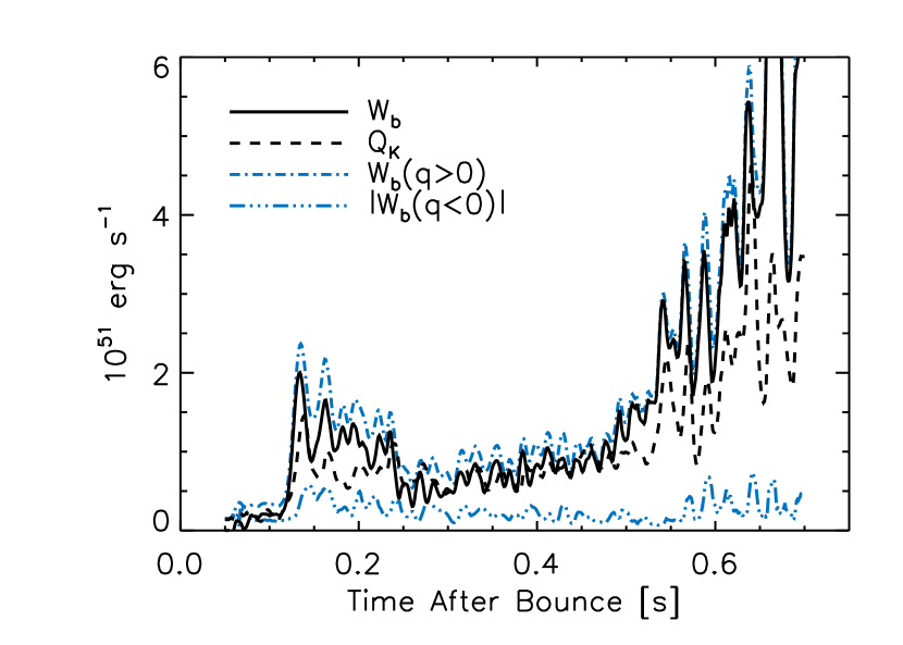
Figure 8.— Buoyancy work integral, $W_{b}$, (solid) and total turbulent dissipation, $Q_{K}$ (dashed), as a function of time after bounce. At all times, the total buoyancy work is roughly balanced by the total turbulent dissipation. $W_{b}(q<0)$ (blue, dot-dashed line) is the buoyancy work for the region where the integrand of $W_{b}$, $q=\langle\rho^{\prime}v_{r}^{\prime}\rangle g_{r}$, is greater than zero, and $|W_{b}(q<0)|$ is buoyancy breaking where $q<0$. At early times, buoyancy breaking contributes significantly to the balance, but is much diminished as the convective motions strengthen near explosion. See § 5 for further discussion.

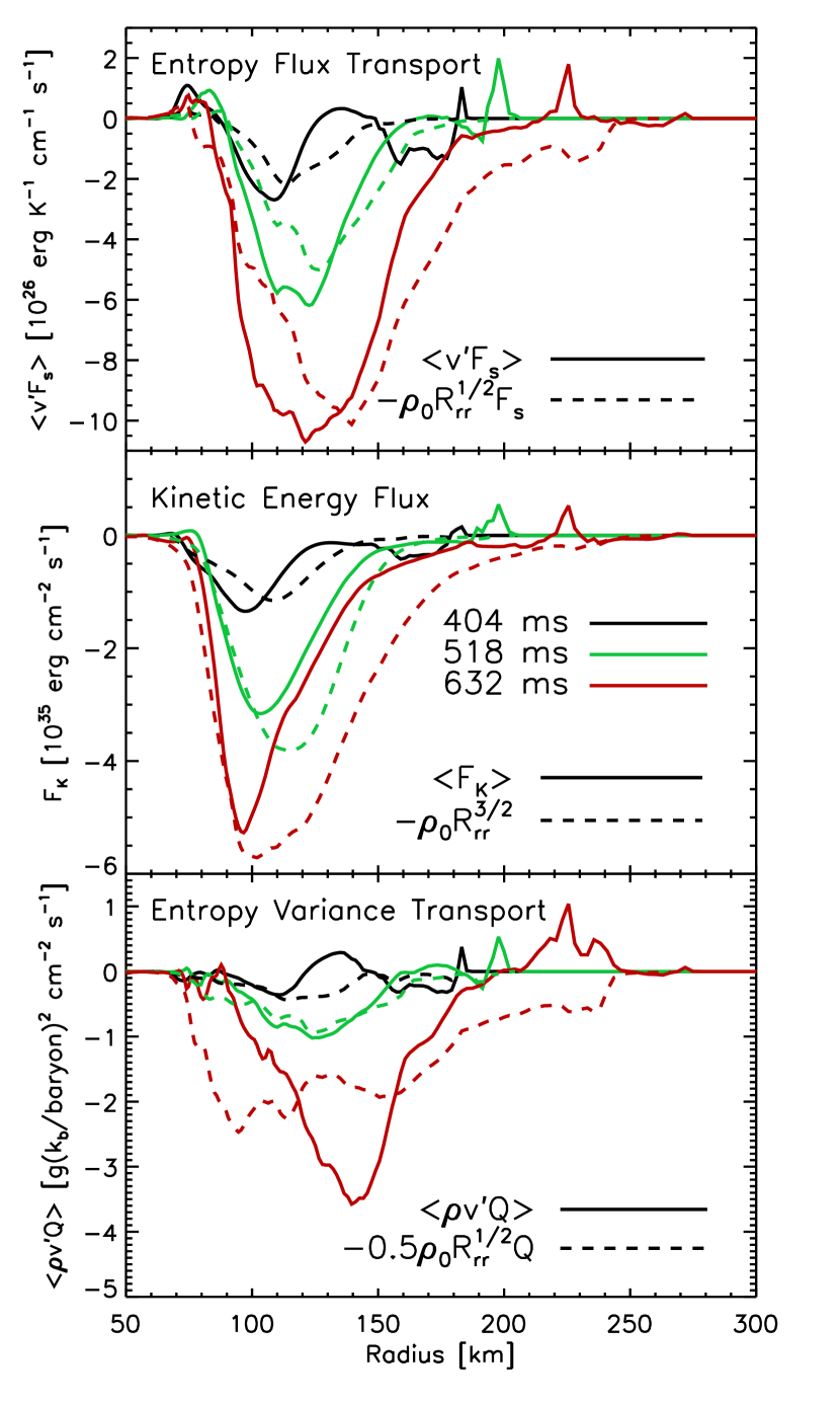
Figure 9.— Comparison of turbulent transport terms (solid lines) to model eqs. (21-23) (dashed lines). This figure is similar to Fig. 4 in presentation. The transport terms are not proportional to the gradient of $R_{rr}$ as the gradient approximation would suggest (Pope, 2000; Launder & Sandham, 2002). Rather, they are proportional to $R_{rr}^{1/2}E_{i}$, where $E_{i}$ is the quantity in question to be transported. This is a consequence of transport by large scale plumes.

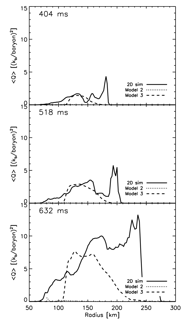
Figure 10.— Radial profile of the entropy variance, $\left<Q\right>$ during the three phases shown in Fig. 1. In this figure, we compare the results of 2D simulations (solid line) with the results of the turbulence models. Only Models 2 & 3 (§4.4 & 4.5) provide any predictions for $\left<Q\right>$, and of these the algebraic model (dashed-line, Model 2) gives the appropriate scale and evolution.

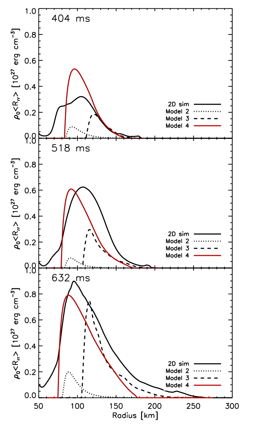
Figure 11.— Radial profile of the radial part of the Reynolds stress, $\left<R_{rr}\right>$ during the three phases shown in Fig. 1. As in Fig. 10, this figure compares the results of 2D simulations (solid lines) with the results of the models presented in sections 4.4-4.6. The 2D results best match the radial profile and the temporal evolution of our global model (red line, Model 4).

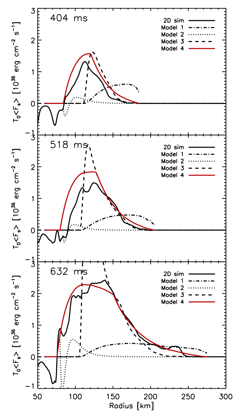
Figure 12.— Radial profile of the enthalpy flux, $T_{0}\left<F_{s}\right>$ during the three phases shown in Fig. 1. This figure compares the results of 2D simulations (solid lines) with the results of the models presented in sections 4.3-4.6. Of these models, only the global model (red line, Model 4) reproduces the scale, profile, and evolution of the 2D simulation.

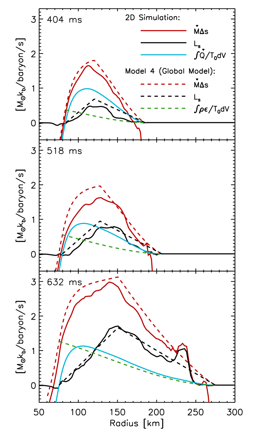
Figure 13.— Radial profiles of entropy change in units of $\dot{M}\Delta s$. The solid lines represent 2D simulation results, and the dashed lines are the results of the global model, Model 4. The integrated neutrino heating and cooling (blue line) and turbulent dissipation (green dot-dashed line) are evaluated from $r$ to the shock radius, $R_{s}$. The modeled entropy difference (red-dashed line) is a sum of the integrated neutrino heating and cooling (blue line), the modeled integrated turbulent dissipation (green-dashed line), and the modeled convective entropy luminosity, $L_{s}$ (green dot-dashed line).The entropy difference derived using the global model (red-dashed line) shows the same scale, radial profile, and temporal evolution as the 2D simulation data (red solid line). Convection ($L_{s}>0$) fills the region where the integrated neutrino heating and cooling (blue line) is greater than zero. The 2D simulated $L_{s}$ profile (black-dashed line) is self-similar and can be modeled by a piecewise linear, pointed hat.

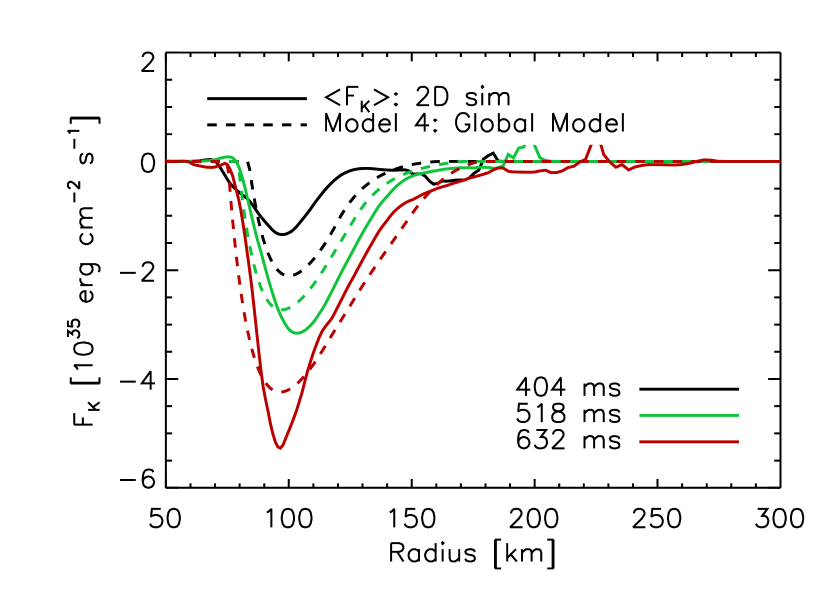
Figure 14.— Convective kinetic energy flux, $F_{K}$, at 404 ms, 518 ms, and 632 ms after bounce as a function of radius. The results of the global model (Model 4, dashed lines) reproduce the scale, general profile, and temporal evolution of the 2D data (solid lines).

6. Turbulence and Conditions for Explosion

In this section, we suggest that the entropy equation, eq. (6), holds the key to understanding the explosion conditions. Furthermore, we use this equation to argue that of all the convective terms, the divergence of the convective entropy flux most affects the critical luminosity for successful explosions. It has been suggested that the critical luminosity condition is equivalent to either a ratio of timescales condition (Thompson, 2000; Janka, 2001; Thompson et al., 2005; Murphy & Burrows, 2008b) or to an ante-sonic condition (Pejcha & Thompson, 2011). In either case, it is the entropy equation, eq. (6), that leads to this result. For example, if we ignore the turbulence terms and integrate the entropy equation over the gain region, then we can derive a ratio of advection to heating timescales

$$\frac{\tau_{\rm{advect}}}{\tau_{\rm{heat}}}\sim\frac{1}{\Delta s}\int^{r_{\rm{gain}}}_{R_{s}}\frac{\dot{Q}}{\dot{m}T}dr\,,$$ (55)

where $\Delta s=s(r_{\rm gain})-s(R_{s})$ is the change in the entropy between the shock ($R_{s}$) and gain ($r_{\rm{gain}}$) radii. Numerical results have confirmed that explosion ensues when this ratio exceeds $\sim$1 (Buras et al., 2006; Scheck et al., 2008; Murphy & Burrows, 2008b; Nordhaus et al., 2010). In the simplest interpretation, this result suggests that explosion occurs roughly when $\Delta s(r)$ exceeds a critical value, $\Delta s_{\rm{crit}}$. Including turbulent terms, the change in entropy as function of radius is

$$\Delta s(r)=-\int^{R_{s}}_{r}\frac{\dot{Q}+\rho_{0}\epsilon}{\dot{m}T}dr-\frac{L_{s}(r)}{\dot{M}}\,,$$ (56)

where $L_{s}(r)=4\pi r^{2}F_{s}(r)$ and recall that $\dot{m}$ and $\dot{M}$ are negative. In our 2D simulations, we find that, of the two turbulent terms in eq. (56), the last term contributes the most entropy change. Therefore, if the time condition is a relevant explosion condition, then the entropy flux is the turbulent correlation that most affects the critical luminosity.

While the timescale condition has proven to be a useful diagnostic for explosions, Pejcha & Thompson (2011) have found a more precise explosion condition in that explosions occur when $c_{s}^{2}/v_{e}^{2}$ exceeds $\sim$ 0.2, where $c_{s}^{2}$ and $v_{e}^{2}$ are the local sound speed and escape velocities squared. They call this new condition the ante-sonic condition and note that it varies by only a few percent when the neutrino luminosity is changed by two orders of magnitude. Over the same range of neutrino luminosities, the timescale ratio at explosion varies from 0.7 to 1.1. In other words, the timescale condition is of order 1, but it varies by $\sim$1.6. Hence, while the timescale ratio is a useful diagnostic relating the most important physical processes, the ante-sonic condition is a more precise (although more obscure) condition for explosion.

Using the integrated form of the entropy equation, eq. (56), we show that the timescale diagnostic and ante-sonic condition are intimately related. The difference in the sound speed between the shock and an arbitrary radius, $r$ is

$$\Delta c_{s}^{2}(r)\approx\frac{P}{\rho_{0}}+\frac{c_{T}^{2}}{c_{V}}\Delta s(r)\,,$$ (57)

where $P$ and $\rho_{0}$ are evaluated at $r$, $c_{T}^{2}=-(T/\rho)(\partial P/\partial T)_{\rho}$ is evaluated at constant density, and $c_{V}=T(\partial s/\partial T)_{V}$ is the specific heat at constant volume. The first term on the R. H. S. of eq. (57) gives the increase in sound speed due to adiabatic compression. The second term represents the change in the sound speed due to changes in entropy given by heating and cooling,

$$-\frac{c_{T}^{2}}{c_{v}}\int^{R_{s}}_{r}\frac{\dot{Q}}{\dot{m}T}dr\,,$$ (58)

and by convection,

$$-\frac{c_{T}^{2}}{c_{v}}\frac{L_{s}}{\dot{M}}\,.$$ (59)

Furthermore, since the second term is proportional to the change in entropy, it is also proportional to the ratio of timescales. Through $\Delta s$, it is apparent that the ante-sonic condition, $c_{s}^{2}/v_{e}^{2}\sim 0.2$, is directly related to the timescale diagnostic.

In a forthcoming paper, we will provide a more thorough discussion of these conditions, how they relate to the critical luminosity for explosions, and how convection affects all three conditions. For now, these analytics reaffirm the supposition in § 3.3 that the convective entropy flux most affects the explosion conditions.

6.1. Turbulence and Explosion Condition: 2D Simulation Results

To see if the ante-sonic condition is consistent with our 2D simulations, we plot $c_{s}^{2}/v_{e}^{2}$ as a function of radius and at four times in Fig. 15. The first three times correspond to the stages shown in Fig. 1 and sample a range of convective strength from weakest at the earliest time to strongest at the latest time. The final time, 700 ms after bounce, corresponds to the time of explosion, which we define as the time when all measures of shock radii (see the top panel in Fig. 7) expand indefinitely. For comparison, we show $c_{s}^{2}/v_{e}^{2}$ of 1D models for these times. The 1D profiles show very little evolution. However, in 2D simulations, the maximum of $c_{s}^{2}/v_{e}^{2}$ is strongly correlated with the strength of convection and the shock radius. At explosion, the peak of $c_{s}^{2}/v_{e}^{2}$ is $\sim$0.2, which is consistent with the explosion condition proposed by Pejcha & Thompson (2011).

It has been argued that convection increases the dwell time in the gain region, which in turn reduces the critical luminosity. Pejcha & Thompson (2011), on the other hand, propose that convection acts to rearrange the flow so that there is less cooling, and this reduced cooling is responsible for lower critical luminosities. The heating and cooling profiles in Fig. 2 and the entropy profiles in Fig. 6 offer a way to investigate the merits of each proposal. Unfortunately, interpretation is somewhat complicated by the fact that the average 2D cooling is less than 1D cooling for some radii and times but is higher for other radii and times. Below $\sim$80 km, 2D cooling is always more than 1D cooling by $\sim$10%. Above this radius, 2D cooling is generally a few percent less than 1D cooling. However, at later times (518 and 632 ms) and above $\sim$120 km, 2D cooling is a few percent larger than 1D again.

However, Fig. 6 shows that the differences in the average cooling between 1D and 2D are small and do not greatly affect the entropy profile. When the convective terms are ignored, the 2D (solid green) and 1D (solid red) entropy profiles are quite similar. Though there are small differences, the differences in average cooling profiles are dwarfed by the effects of including the convective terms in the entropy equation (dot-dashed green curve). Therefore, it is unlikely that changes in the average cooling between 1D and 2D lead to the reduction in the critical luminosity. Rather, as we argue in §6 it is more likely that the divergence of the convective entropy flux is responsible for the extra entropy, higher sound speeds, and a reduction in the critical luminosity.

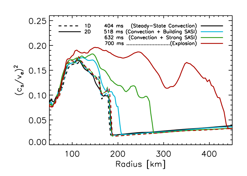
Figure 15.— Ratio of sound speed and escape velocity squared as a function of radius. The four times shown correspond to the three phases in Fig. 1 (404, 518, and 632 ms after bounce) and explosion (700 ms after bounce). As convection increases in vigor, the maximum in this ratio increases until it reaches $\sim$0.2 at the time of explosion. These results are consistent with the ante-sonic condition proposed by Pejcha & Thompson (2011).

7. Conclusion

Recent simulations of CCSNe indicate that turbulence reduces the critical neutrino luminosity for successful explosions. This suggests that a theory for successful explosions requires a theoretical framework for turbulence and its influence on the critical luminosity. In this paper, we develop a foundation for this framework, which is represented by the following results:

• We derive the exact steady-state equations for the background and turbulent flow.

• We identify the convective terms that most influence the conditions for successful explosions.

• We have shown that without turbulence, entropy profiles of 2D simulations would be nearly identical to 1D and that the convective terms entirely make up the difference.

• This further motivates the need to understand turbulence in the context of CCSNe. To this end, we cull the literature for a broad sample of turbulence models, but after a quantitative comparison with 2D simulations, we find that none adequately reproduce the global turbulent profiles. These single-point models fail because they use local closure approximations, even though buoyantly driven turbulence is a global phenomenon.

• Motivated by the necessity for an alternate approach, we propose an original model for turbulence which incorporates global properties of the flow. This global model has no free parameters; instead the scale (or parameters) of convection are constrained by global conservation laws. Furthermore, this model accurately reproduces the turbulence profiles and evolution of 2D CCSN simulations.

Using Reynolds decomposition, we derive steady-state averaged equations for the background flow and turbulent correlations, eqs. (7-10). These equations naturally incorporate effects that are important in the CCSN problem such as steady-state accretion, neutrino heating and cooling, non-zero entropy gradients, buoyant driving, turbulent transport, and dissipation. We validate these equations using 2D CCSN simulations. For example, we integrate the entropy equation with and without the convective terms (see Fig. 6). If we neglect the turbulence terms, then we recover the 1D entropy profile. The difference between the 1D and 2D entropy profiles is entirely accounted for by the physics of turbulence.

Turbulence equations require closure models, but these closure models depend upon the macroscopic properties of the flow. To derive a closure model that is appropriate for CCSNe, we compare a representative sample of closure models in the literature with 2D simulations. Motivated by the failure of these models, we have developed an original closure model. While the models culled from the literature are single-point closure models and use local closure approximations, our model is distinguished by using global properties of the flow for closure. This global model is further distinguished by reproducing the scale, profile, and evolution of turbulence in 2D simulations.

The single-point models use local turbulent correlations to derive closure relations for the higher order correlations. Convection is inherently a global phenomenon, and so while it is possible to model the higher-order correlations with local approximations in some locations, these models can be factors off in other locations. Given the stiff nature of the Reynolds-averaged equations, these errors, even if modest, can lead to significantly flawed global solutions. Rather than relying on these local models, we integrate the turbulence equations and derive global constraints based on conservation laws. We propose that nonlocal turbulent transport relaxes the turbulent profiles to satisfy these global constraints. This relaxation combined with the similarity of buoyant driving, entrainment, and dissipation leads to self-similar profiles for the most important turbulent correlations. In Model 4, we construct a global model in which we define these self-similar profiles and use global conservation laws to determine their scales. Locally, we use the differential form of the conservation equations to derive the remaining profiles.

Our model represents a new approach to turbulence modeling, so we elucidate the assumptions and features that distinguish it from previous models. Single point closure models try to employ universal characteristics on the smallest scales to close the problem. We are approaching this from the other direction. The nonlocal nature of plume dominated convection leads us to assume universality on the largest scales and a minimum set of global profiles to close the problem. These two approaches are complimentary. Assuming universality on the smallest scales lends itself to dynamic simulations, while the global approach lends itself very well to steady-state problems.

The general strategy that we employ is to establish some general characteristic of turbulence and use global conservation laws to constrain the scale. For now, we identify the apparent self-similar profiles as the general characteristic. In fact, these self-similar profiles are motivated by the generic properties of plume dominated flows and the results of 2D CCSN and 3D stellar convection simulations. In the future, we hope to identify a more fundamental characteristic and physical assumption that leads to these profiles. But until then, our global model is the only model that consistently gives the correct scale, profile, and temporal evolution for the convective kinetic energy flux, $F_{K}$, and entropy flux, $F_{s}$. The strongest validation of this model is Fig. 13, in which we reproduce the entire entropy profile of 2D simulations.

In preparation to deriving the reduced critical luminosity, we identify the turbulent terms that most influence the conditions for explosion. Three explosion conditions have been explored in the literature. Burrows & Goshy (1993) proposed a critical neutrino luminosity for successful explosions and Murphy & Burrows (2008b) used 1D and 2D simulations to show that this condition indeed separates steady state accretion from dynamic explosions. Alternatively, it has been suggested that explosions occur when the advection timescale through the gain region exceeds the heating timescale. More recently, Pejcha & Thompson (2011) suggest an ante-sonic condition in which explosions occur once $c^{2}_{s}/v^{2}_{e}$ exceeds 0.2. In Fig. 15, we show that in 2D simulations, $c^{2}_{s}/v^{2}_{e}$ indeed reaches 0.2 at explosion. Moreover, using our Reynolds-averaged equations, we show that the timescale and the ante-sonic conditions are intimately related, and in both conditions, convection aides explosion because turbulence raises the entropy by a term proportional to $L_{s}/\dot{M}$.

In summary, our global turbulence model contains no free parameters, is globally self-consistent, accurately reproduces the mean-field properties of 2D CCSN turbulence, and promises to explain the reduction in the critical luminosity. Despite these successes, closure approximations generically depend upon the properties of the macroscopic flow, making them case-dependent. Hence, it is unclear to what extent this turbulence model can accurately describe 3D turbulence, especially in the presence of rapid rotation and/or magnetic fields.

Preliminary work (Thompson et al., 2005; Yamasaki & Yamada, 2005; Burrows et al., 2007a) hints that large rotation rates and magnetic field strengths could aid explosion, but it is uncertain how modest values would alter turbulence and its effects on explosion. Under the most extreme rotation rates and/or magnetic fields, the flow can be severely distorted from spherical symmetry (e.g. jets, Burrows et al., 2007a). In these conditions, it is best to study the role of rotation and magnetic fields on turbulence using multi-dimensional simulations. On the other hand, for mild rotation and magnetic fields, the Reynolds decomposition framework employed in this paper can be applied straightforwardly: mild rotational effects can be included by retaining off-diagonal Reynolds stress terms (e.g., Garaud et al., 2010) and applying Reynolds decomposition to ideal MHD introduces terms associated with the fluctuations of magnetic fields such as Maxwell stresses and Ohmic heating (e.g., Ogilvie, 2003; Pessah et al., 2006). However, these analyses are beyond the scope of this paper, so for now, we comment on the reliability of our global turbulence model for 3D CCSN turbulence.

Even though 2D and 3D turbulence are known to behave differently, the global turbulence model reproduces the turbulent characteristics of 2D CCSN and 3D stellar evolution simulations. We suspect, but have not proven, that this is a testament to the global nature of the turbulence model. Though encouraging, there is no guarantee that the model will work so well for 3D CCSN simulations. Therefore, a reliable turbulence closure model will require comparison with 3D simulations. In 2D simulations, steady-state is a valid assumption. However, differences in the plume structure of 3D turbulence could lead to more efficient heating, which in turn could necessitate including time-dependent terms in the turbulence equations. The global nature of turbulence and the similarity of driving and dissipation should lead to self-similar profiles in both 2D and 3D turbulence. However, the exact profiles may differ. Whether any of these differences will affect closure approximations is uncertain. Only comparison with 3D simulations can clear up this matter.

References

- Arnett et al. (2009) Arnett, D., Meakin, C., & Young, P. A. 2009, ApJ, 690, 1715
- Bethe & Wilson (1985) Bethe, H. A., & Wilson, J. R. 1985, ApJ, 295, 14
- Blondin et al. (2003) Blondin, J. M., Mezzacappa, A., & DeMarino, C. 2003, ApJ, 584, 971
- Bruenn (1985) Bruenn, S. W. 1985, ApJS, 58, 771
- Bruenn (1989) —. 1989, ApJ, 340, 955
- Buras et al. (2003) Buras, R., Rampp, M., Janka, H.-T., & Kifonidis, K. 2003, Physical Review Letters, 90, 241101
- Buras et al. (2006) —. 2006, A&A, 447, 1049
- Burrows et al. (2007a) Burrows, A., Dessart, L., Livne, E., Ott, C. D., & Murphy, J. 2007a, ApJ, 664, 416
- Burrows & Goshy (1993) Burrows, A., & Goshy, J. 1993, ApJ, 416, L75+
- Burrows et al. (1995) Burrows, A., Hayes, J., & Fryxell, B. A. 1995, ApJ, 450, 830
- Burrows et al. (2006) Burrows, A., Livne, E., Dessart, L., Ott, C. D., & Murphy, J. 2006, ApJ, 640, 878
- Burrows et al. (2007b) —. 2007b, ApJ, 655, 416
- Canuto (1993) Canuto, V. M. 1993, ApJ, 416, 331
- Cattaneo et al. (1991) Cattaneo, F., Brummell, N. H., Toomre, J., Malagoli, A., & Hurlburt, N. E. 1991, ApJ, 370, 282
- Chandrasekhar (1961) Chandrasekhar, S. 1961, Hydrodynamic and hydromagnetic stability, ed. Chandrasekhar, S.
- Daly & Harlow (1970) Daly, B. J., & Harlow, F. H. 1970, Physics of Fluids, 13, 2634
- Dessart et al. (2008) Dessart, L., Burrows, A., Livne, E., & Ott, C. D. 2008, ApJ, 673, L43
- Fernández & Thompson (2009) Fernández, R., & Thompson, C. 2009, ApJ, 703, 1464
- Foglizzo (2009) Foglizzo, T. 2009, ApJ, 694, 820
- Foglizzo & Tagger (2000) Foglizzo, T., & Tagger, M. 2000, A&A, 363, 174
- Garaud et al. (2010) Garaud, P., Ogilvie, G. I., Miller, N., & Stellmach, S. 2010, MNRAS, 407, 2451
- Janka (2001) Janka, H.-T. 2001, A&A, 368, 527
- Janka & Müller (1995) Janka, H.-T., & Müller, E. 1995, ApJ, 448, L109
- Kippenhahn & Wiegert (1990) Kippenhahn, R., & Wiegert, A. 1990, Stellar Structure and Evolution (Berlin Heildelberg: Springer-Verlag)
- Kitaura et al. (2006) Kitaura, F. S., Janka, H.-T., & Hillebrandt, W. 2006, A&A, 450, 345
- Launder & Sandham (2002) Launder, B. E., & Sandham, N. D. 2002, Closure Strategies for Turbulent and Transitional Flows (Cambridge: Cambridge University Press)
- Li et al. (2010) Li, W., Leaman, J., Chornock, R., Filippenko, A. V., Poznanski, D., Ganeshalingam, M., Wang, X., Modjaz, M., Jha, S., Foley, R. J., & Smith, N. 2010, ArXiv e-prints
- Liebendörfer et al. (2001a) Liebendörfer, M., Mezzacappa, A., & Thielemann, F.-K. 2001a, Phys. Rev. D, 63, 104003
- Liebendörfer et al. (2001b) Liebendörfer, M., Mezzacappa, A., Thielemann, F.-K., Messer, O. E., Hix, W. R., & Bruenn, S. W. 2001b, Phys. Rev. D, 63, 103004
- Liebendörfer et al. (2005) Liebendörfer, M., Rampp, M., Janka, H.-T., & Mezzacappa, A. 2005, ApJ, 620, 840
- Lorimer et al. (2006) Lorimer, D. R., Faulkner, A. J., Lyne, A. G., Manchester, R. N., Kramer, M., McLaughlin, M. A., Hobbs, G., Possenti, A., Stairs, I. H., Camilo, F., Burgay, M., D’Amico, N., Corongiu, A., & Crawford, F. 2006, MNRAS, 372, 777
- Marek & Janka (2007) Marek, A., & Janka, H. . 2007, ArXiv e-prints, 708
- Marek & Janka (2009) Marek, A., & Janka, H.-T. 2009, ApJ, 694, 664
- Mazurek (1982) Mazurek, T. J. 1982, ApJ, 259, L13
- Meakin & Arnett (2007) Meakin, C. A., & Arnett, D. 2007, ApJ, 667, 448
- Meakin & Arnett (2010) Meakin, C. A., & Arnett, W. D. 2010, Ap&SS, 328, 221
- Murphy & Burrows (2008a) Murphy, J. W., & Burrows, A. 2008a, ApJS, 179, 209
- Murphy & Burrows (2008b) —. 2008b, ApJ, 688, 1159
- Murphy et al. (2009) Murphy, J. W., Ott, C. D., & Burrows, A. 2009, ApJ, 707, 1173
- Nordhaus et al. (2010) Nordhaus, J., Burrows, A., Almgren, A., & Bell, J. 2010, ApJ, 720, 694
- O’Connor & Ott (2011) O’Connor, E., & Ott, C. D. 2011, ApJ, 730, 70
- Ogilvie (2003) Ogilvie, G. I. 2003, MNRAS, 340, 969
- Ohnishi et al. (2006) Ohnishi, N., Kotake, K., & Yamada, S. 2006, ApJ, 641, 1018
- Pejcha & Thompson (2011) Pejcha, O., & Thompson, T. A. 2011, ArXiv e-prints
- Pessah et al. (2006) Pessah, M. E., Chan, C.-k., & Psaltis, D. 2006, Phys. Rev. Lett., 97, 221103
- Plate et al. (1997) Plate, D. C., Fedorovich, E. E., Viegas, D. X., & Wyngaard, J. C., eds. 1997, Buoyant Convection in Geophysical Flows, NATO ASI Series (Dordrecht, The Netherlands: Kluwer Academic Publishers)
- Pope (2000) Pope, S. B. 2000, Turbulent Flows (New York: Cambridge University Press)
- Rampp & Janka (2002) Rampp, M., & Janka, H.-T. 2002, A&A, 396, 361
- Rieutord & Zahn (1995) Rieutord, M., & Zahn, J.-P. 1995, A&A, 296, 127
- Scheck et al. (2008) Scheck, L., Janka, H.-T., Foglizzo, T., & Kifonidis, K. 2008, A&A, 477, 931
- Suwa et al. (2010) Suwa, Y., Kotake, K., Takiwaki, T., Whitehouse, S. C., Liebendörfer, M., & Sato, K. 2010, PASJ, 62, L49+
- Thompson (2000) Thompson, C. 2000, ApJ, 534, 915
- Thompson et al. (2003) Thompson, T. A., Burrows, A., & Pinto, P. A. 2003, ApJ, 592, 434
- Thompson et al. (2005) Thompson, T. A., Quataert, E., & Burrows, A. 2005, ApJ, 620, 861
- Turner (1973) Turner, J. S. 1973, Buoyancy Effects in Fluids (Cambridge: Cambridge University Press)
- Weinberg & Quataert (2008) Weinberg, N. N., & Quataert, E. 2008, MNRAS, 387, L64
- Wilcox (2006) Wilcox, D. C. 2006, Turbulence Modeling for CFD, 3rd edn. (La Canada, California: DCW Industries, Inc.)
- Woosley & Heger (2007) Woosley, S. E., & Heger, A. 2007, Phys. Rep., 442, 269
- Yamasaki & Yamada (2005) Yamasaki, T., & Yamada, S. 2005, ApJ, 623, 1000
- Yamasaki & Yamada (2006) —. 2006, ApJ, 650, 291