The Cosmological Impact of Luminous TeV Blazars I:
Implications of Plasma Instabilities for the Intergalactic Magnetic
Field and Extragalactic Gamma-Ray Background
Abstract
Inverse-Compton cascades initiated by energetic gamma rays () enhance the GeV emission from bright, extragalactic TeV sources. The absence of this emission from bright TeV blazars has been used to constrain the intergalactic magnetic field (IGMF), and the stringent limits placed upon the unresolved extragalactic gamma-ray background (EGRB) by Fermi has been used to argue against a large number of such objects at high redshifts. However, these are predicated upon the assumption that inverse-Compton scattering is the primary energy-loss mechanism for the ultra-relativistic pairs produced by the annihilation of the energetic gamma rays on extragalactic background light photons. Here we show that for sufficiently bright TeV sources (isotropic-equivalent luminosities ) plasma beam instabilities, specifically the “oblique” instability, present a plausible mechanism by which the energy of these pairs can be dissipated locally, heating the intergalactic medium. Since these instabilities typically grow on timescales short in comparison to the inverse-Compton cooling rate, they necessarily suppress the inverse-Compton cascades. As a consequence, this places a severe constraint upon efforts to limit the IGMF from the lack of a discernible GeV bump in TeV sources. Similarly, it considerably weakens the Fermi limits upon the evolution of blazar populations. Specifically, we construct a TeV-blazar luminosity function from those objects presently observed and find that it is very well described by the quasar luminosity function at , shifted to lower luminosities and number densities, suggesting that both classes of sources are regulated by similar processes. Extending this relationship to higher redshifts, we show that the magnitude and shape of the EGRB above is naturally reproduced with this particular example of a rapidly evolving TeV-blazar luminosity function.
keywords:
BL Lacertae objects: general – gamma rays: general – instabilities – magnetic fields – plasmas – radiative mechanisms: non-thermal1 Introduction
lccccccccccl\tabletypesize
\tablecaptionList of TeV Sources with Measured Spectral Properties in Decreasing – Flux Order
\tablehead
\colheadName &
\colhead
\colhead \tablenotemarka
\colhead \tablenotemarkb
\colhead \tablenotemarkc
\colhead \tablenotemarkd
\colhead \tablenotemarke
\colhead \tablenotemarkf
\colhead \tablenotemarkg
\colhead \tablenotemarkh
\colheadClass \tablenotemarki
\colheadReference
\startdataMkn 421 & 0.030 129 68 1 3.32 45.6 3.15 H Chandra et al. (2010)
1ES 1959+650 0.047 201 78 1 3.18 45.9 2.90 85 H Aharonian et al. (2003)
1ES 2344+514 0.044 190 120 0.5 2.95 45.0 2.82 H Albert et al. (2007c)
Mkn 501 \tablenotemarkj 0.034 150 8.7 1 2.58 85 44.4 2.39 H Huang et al. (2009)
3C 279 0.536 2000 520 0.2 4.11 68 46.9 2.53 2.0 Q MAGIC Collaboration et al. (2008a)
PKS 2155-304 0.116 490 1.81 1 3.53 64 45.4 2.75 H HESS Collaboration et al. (2010)
PG 1553+113 46.8 0.3 4.46 41 H Aharonian et al. (2008b)
W Comae 0.102 430 20 0.4 3.68 31 44.9 3.41 I Acciari et al. (2009b)
3C 66A 0.444 1700 40 0.3 4.1 28 46.3 2.43 13 I Acciari et al. (2009c)
1ES 1011+496 0.212 870 200 0.2 4 26 45.5 3.66 H Albert et al. (2007b)
1ES 1218+304 \tablenotemarkj 0.182 750 11.5 0.5 3.07 24 45.4 2.37 H Acciari et al. (2010a)
Mkn 180 0.045 190 45 0.3 3.25 20 44.0 3.17 H Albert et al. (2006)
1H 1426+428 0.129 540 2 1 2.6 20 45.0 1.71 H Aharonian et al. (2002)
RGB J0710+591 \tablenotemarkj 0.125 520 1.36 1 2.69 15 44.8 1.83 H Acciari et al. (2010c)
1ES 0806+524 0.138 580 6.8 0.4 3.6 10 44.7 3.21 H Acciari et al. (2009a)
RGB J0152+017 \tablenotemarkj 0.080 340 0.57 1 2.95 8.5 44.1 2.45 H Aharonian et al. (2008a)
1ES 1101-232 \tablenotemarkj 0.186 770 0.56 1 2.94 8.2 44.9 1.50 H Aharonian et al. (2007a)
1ES 0347-121 \tablenotemarkj 0.185 770 0.45 1 3.1 8.2 44.9 1.67 H Aharonian et al. (2007b)
IC 310 0.019 83 1.1 1 2.0 8.1 42.8 1.90 H Aleksić et al. (2010)
PKS 2005-489 0.071 300 0.1 1 4.0 8.0 44.0 3.56 H Aharonian et al. (2005)
MAGIC J0223+430 – – 17.4 0.3 3.1 7.6 – – R Aliu et al. (2009)
1ES 0229+200 \tablenotemarkj 0.140 590 0.7 1 2.5 6.4 44.5 1.51 H Aharonian et al. (2007c)
PKS 1424+240 51 0.2 3.8 6.3 4.0 I Acciari et al. (2010b)
M87 0.0044 19 0.74 1 2.31 5.9 41.4 2.29 R Acciari et al. (2008)
BL Lacertae 0.069 290 0.3 1 3.09 5.4 43.8 2.67 L Albert et al. (2007a)
H 2356-309 0.165 690 0.3 1 3.09 5.4 44.6 1.86 H Aharonian et al. (2006)
PKS 0548-322 \tablenotemarkj 0.069 290 0.3 1 2.86 4.0 43.7 2.44 H Aharonian et al. (2010)
Centaurus A 0.0028 12 0.245 1 2.73 2.8 40.7 2.72 R Raue et al. (2010)
\enddata\tablenotetextaComoving distance in units of
\tablenotetextbNormalization of the observed photon spectrum that we assume to be of the form , in units of
\tablenotetextcEnergy at which we normalize the spectrum, in units of
\tablenotetextdObserved spectral index at
\tablenotetexteIntegrated energy flux between and , in units of
\tablenotetextfInferred isotropic integrated luminosity between and , in units of
\tablenotetextgInferred intrinsic spectral index at
\tablenotetexthTime delay after which plasma beam instabilities dominate inverse-Compton cooling, in units of
\tablenotetextiH, I, L, Q, and R correspond to high-energy,
intermediate-energy, low-energy peaked BL Lacs, flat spectrum radio quasars, and radio galaxies of Faranoff-Riley Type I (FR I), respectively.
\tablenotetextjUsed to place limits upon the IGMF
Imaging atmospheric Cerenkov telescopes, such as H.E.S.S., VERITAS, and MAGIC,111High Energy Stereoscopic System, Major Atmospheric Gamma Imaging Cerenkov Telescope, Very Energetic Radiation Imaging Telescope Array System. have opened the very-high energy gamma-ray (VHEGR, ) sky, finding a Universe populated by a variety of energetic, VHEGR sources. While the majority of observed VHEGR sources are Galactic in origin (e.g., supernova remnants, etc.), the extragalactic contribution is dominated by a subset of blazars. There are presently 46 extragalactic TeV sources known222See http://www.mppmu.mpg.de/rwagner/sources/ for an up-to-date list., of which 28 have well defined spectral energy distributions (SEDs), and are collected in Table 1. Of these 28 well-studied objects, 24 are blazars, implying that blazars make up an overwhelming majority of the bright VHEGR sources.
All of the extragalactic VHEGR emitters are relatively nearby, with generally, and typical. This is a result of the large opacity of the Universe to TeV photons, which annihilate upon soft photons in the extragalactic background light (EBL), producing pairs (see, e.g., Gould & Schréder, 1967; Salamon & Stecker, 1998; Neronov & Semikoz, 2009). Typical mean free paths of VHEGRs range from to depending upon gamma-ray energy and source redshift, and thus the absence of high-redshift VHEGR sources is not unexpected.
The pairs produced by VHEGR annihilation are necessarily ultrarelativistic, with typical Lorentz factors of –. The standard assumption is that these pairs lose energy almost exclusively through inverse-Compton scattering the cosmic microwave background (CMB) and EBL. When the up-scattered gamma-ray is itself a VHEGR the process repeats, creating a second generation of pairs and up-scattering additional photons. The result is an inverse-Compton cascade (ICC) depositing the energy of the original VHEGR in gamma-rays with energies . This places the ICC gamma rays in the LAT bands of Fermi, and thus Fermi has played a central role in constraining the VHEGR emission of high-redshift blazars.
Based upon Fermi observations of TeV sources, a number of authors have now published estimated lower bounds upon the intergalactic magnetic field (IGMF; see, e.g., Neronov & Vovk, 2010; Tavecchio et al., 2010, 2011; Dermer et al., 2011; Taylor et al., 2011; Takahashi et al., 2012; Dolag et al., 2011). Typical numbers range from to , with the latter values being of astrophysical interest in the context of the formation of galactic fields333After contraction and a handful of windings, nG field strengths can be produced from an IGMF of .. These limits on the IGMF arise from the lack of the GeV bump associated with the ICC of the blazar TeV emission, presumably due to the resulting pairs being deflected significantly under the action of the IGMF itself. The wide range in the estimates upon the minimum IGMF is due primarily to different assumptions about the TeV blazar duty cycle.
Fermi has also provided the most precise estimate of the unresolved extragalactic gamma-ray background (EGRB) for energies between and . Since ICCs reprocess the VHEGR emission of distant sources into this band, this has been used to constrain the evolution of the luminosity density of VHEGR sources (see, e.g., Narumoto & Totani, 2006; Kneiske & Mannheim, 2008; Inoue & Totani, 2009; Venters, 2010). Generally, it has been found that these cannot have exhibited the dramatic rise in numbers by – seen in the quasar distribution. That is, the comoving number of blazars must have remained essentially fixed, at odds with both the physical picture underlying these systems and with the observed evolution of similarly accreting systems, i.e., quasars.
Both of these conclusions depend critically upon ICCs dominating the evolution of the ultra-relativistic pairs. However, as we will show, the pairs constitute a cold, highly collimated plasma beam moving through a dense, stationary background, both of which are susceptible to collective plasma phenomena. Such beams are notoriously unstable; for instance, equal density beams typically lose a significant fraction of their energy after propagating distances measured in plasma skin depths of the background plasma. If the VHEGR-generated pairs suffer a similar fate while propagating through the intergalactic medium (IGM), the cooling of the pairs would be dominated by plasma instabilities, thereby quenching the ICCs.
Here we present a plausible alternative mechanism by which the energy in the ultra-relativistic pairs can be extracted. While a variety of potential plasma beam instabilities exist, we find that the most relevant for the VHEGR-produced pair beams is the “oblique” instability (Bret et al., 2004, 2005a; Bret, 2009; Bret et al., 2010b; Lemoine & Pelletier, 2010). This is a more virulent cousin of the commonly discussed Weibel and two stream instabilities.
In Section 2 we discuss the formation and properties of the ultra-relativistic pair beam, including limits upon its temperature and density. Section 3 presents growth rates for a variety of plasma instabilities, including the oblique instability. Particular attention is paid to if and when plasma instabilities dominate inverse Compton as a means to dissipate the kinetic energy of the pairs. The resulting implications for studies of the IGMF are described in Section 4, including how such efforts might mitigate the systematic uncertainties arising from plasma cooling. The evolution of the luminosity function of VHEGR-emitting blazars is discussed in Section 5, in which we construct a blazar luminosity function based upon that of quasars which is consistent with current TeV source populations and the Fermi estimates of the EGRB. Finally, conclusions are contained in Section 6.
This is the first in a series of three papers that discuss the potential cosmological impact of the TeV emission from blazars. Here we provide a plausible mechanism for the local dissipation of the VHEGR luminosity of bright gamma-ray sources. In addition to the particular consequences this has for studies of high-energy gamma-ray phenomenology, it also provides an novel heating process within the IGM. Chang et al. (2012, hereafter Paper II) estimates the magnitude of the new heating term, describes the associated modifications to the thermal history of the IGM, and shows how this can explain some recent observations of the Ly forest. Pfrommer et al. (2012, hereafter Paper III) considers the impact the new heating term has upon the structure and statistics of galaxy clusters and groups, and upon the ages and properties of dwarf galaxies throughout the Universe, generally finding that blazar heating can help explain outstanding questions in both cases. An additional follow-up paper by Puchwein et al. (2011) shows that when combined with most recent estimates of the evolving photoionizing background and hydrodynamic simulations of cosmological structure formation, the heating by blazars results in excellent quantitative agreement with observations of the mean transmission, one- and two-point statistics, and line width distribution of high-redshift Ly forest spectra. In particular, these successes depends upon the peculiar properties of the blazar heating via the dissipation of plasma instabilities.
For all of the calculations presented below we assume the WMAP7 cosmology with , , , and (Komatsu et al., 2011).
2 The Fate of Very High Energy Gamma Rays and the Properties of the Resulting Pair Beam
2.1 Propagation and Absorption of Very High-Energy Gamma rays
Sources of VHEGRs are necessarily attenuated by the production of pairs upon interacting with the EBL. Namely, when the energies of the gamma ray () and the EBL photon () exceed the rest mass energy of the pair in the center of mass frame, i.e., , where is the relative angle of propagation in the lab frame, an pair can be produced with Lorentz factor (Gould & Schréder, 1967). The optical depth the Universe presents to high-energy gamma rays depends solely upon the energy of the gamma ray and the evolving spectrum of the EBL444As a consequence, careful studies of the absorption of high-energy gamma rays from extragalactic sources has been suggested as a way to probe the EBL (see, e.g., Gould & Schréder, 1967; Stecker et al., 1992; Oh, 2001).. Detailed estimates for the EBL spectrum and its evolution have produced an estimated mean free path of TeV photons of
| (1) |
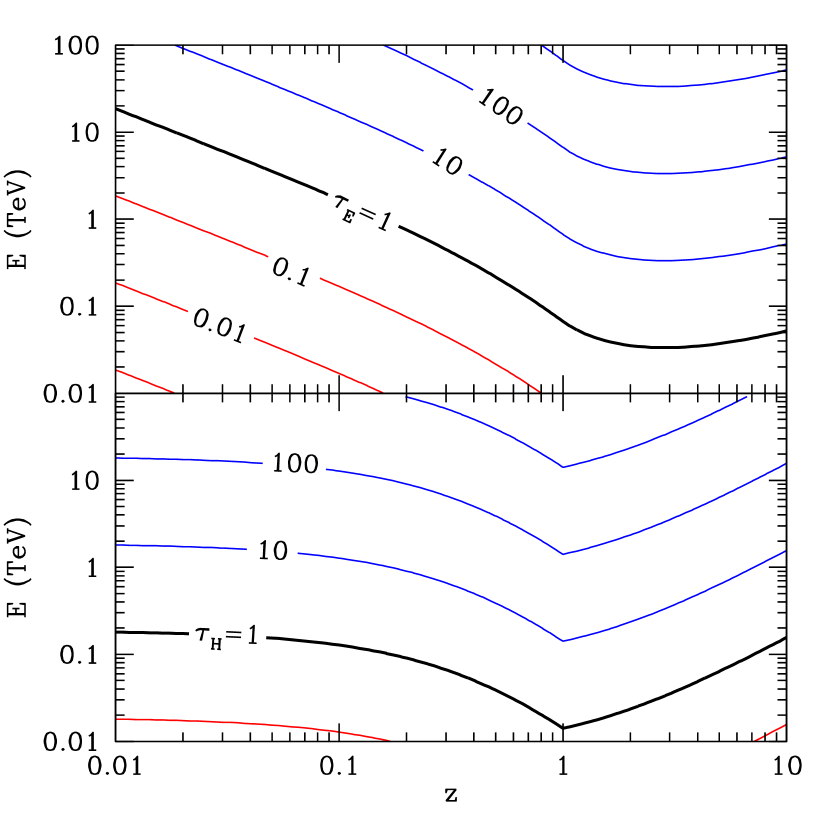
where the redshift evolution is due to that of the EBL alone, is dependent predominately upon the star formation history, and for and for (Kneiske et al., 2004; Neronov & Semikoz, 2009)555Despite the fact that the EBL contribution from starbursts peaks at and declines rapidly afterward, galaxies and Type 1 active galactic nuclei compensate for the lost flux until . See, for example, Figure 3 from Franceschini et al. (2008).. The resulting optical depth to VHEGRs emitted with energy from an object located at is
| (2) |
(in which is the Hubble factor), is shown in the top panel of Figure 1.666Note that the optical depth experienced by a photon that is observed to have energy is given by . From this it is evident that above the Universe is optically thick to sources at (cf. Franceschini et al., 2008). A related, and perhaps more appropriate measure of the optical depth is that across a Hubble length, , shown in the bottom panel of Figure 1, providing a sense of how opaque the Universe is as a function of redshift. In all cases it is clear that at photons will pair-produce on the EBL for . In the future this may not be the case, since for sufficiently small , decreases with decreasing due to the dramatic decrease in the EBL photon density associated with both the Hubble expansion and the slowing of star formation.
2.2 Temperature of the Ultra-Relativistic Pair Beam
The pairs produced by the TeV gamma rays are ultra-relativistic, with typical Lorentz factors of . They also necessarily constitute a cold, highly anisotropic, dilute beam propagating through the IGM. This follows immediately from the intergalactic distances traversed by the gamma rays and the comparatively small EBL photon energies (as seen in the IGM frame). Here we estimate the properties of this plasma beam.
The momentum dispersion of the resulting pairs is set by the gamma-ray spectrum, geometry of the TeV source, distribution of the EBL photons, and heating due to pair production. Of these, only the last plays a significant role in setting the transverse momentum dispersion.777The contribution to the transverse momentum dispersion from the finite source size, due to the slightly different orientations of photons from opposing sides of the TeV emission region of size , is . With , implied by the X-ray variability timescales (Tramacere et al., 2009; Abdo et al., 2010d), this gives . Similarly, since the creation of pairs is dominated by EBL photons near the pair-production threshold, the typical energy of the relevant EBL photons is roughly (i.e., twice the threshold value for transverse EBL photons), and thus . The center-of-mass frame, i.e., the “beam frame”, momentum dispersion resulting from pair production is roughly . This results in an IGM-frame transverse momentum dispersion of . With , the temperature888The temperature of an anisotropic particle distribution is inherently ill defined. Here we identify a temperature with the momentum dispersion of the beam using the drifting Maxwell-Jüttner distribution employed by Bret et al. (2010a) (eq. 1 therein). associated with this transverse momentum dispersion is
| (3) |
Since the transverse momentum dispersion of the pairs is much smaller than that associated with the bulk motion of the beam (i.e., since ), we may safely assume that the beam is transversely kinematically cold.
2.3 Density of the Ultra-Relativistic Pair Beam in General
The density of the pair beam at a given point within the IGM is set by the rate at which pairs are produced, duration of the TeV emission, advection of the pairs through the IGM, and the processes by which they lose their kinetic energy. That is, the evolution of the density of pairs per unit Lorentz factor, , is governed by the Boltzmann equation:
| (4) |
where the left-hand side assumes all the pairs are moving away from the TeV source relativistically ( and ), and the right-hand side corresponds to pair production. Generally, we may neglect advection, which alters over timescales of , much longer than any relevant timescale of interest here (i.e., may be neglected). Furthermore, for most of the potential sources we will consider (primarily TeV blazars) we will assume that the duration of the TeV emission is sufficiently long that reaches a steady state (i.e., ). In this case, we have .
Making further progress requires us to define the spectrum of the pairs, which itself depends upon the spectrum of the gamma rays and the energy dependence of the cooling processes. Nevertheless, we may obtain an estimate of the beam density in the vicinity of a given Lorentz factor, , by setting .
The source term is given by twice (since each gamma-ray produces two leptons) the rate at which high-energy gamma rays with energy annihilate within the region of interest, i.e., , where is the gamma-ray number flux, with units of . Thus, upon defining a cooling rate , we have
| (5) |
i.e., the density of pairs of a given energy is determined by balancing cooling and pair creation.
Generally, is a function of energy and beam density, as well as external factors (e.g., seed photon density, IGM density, etc.). Thus this gives a non-linear algebraic equation to solve for , the particulars of which depend upon the various mechanisms responsible for extracting the bulk energy of the beam. In practice, given expressions for , associated with the processes discussed in following section, we solve Equation (5) numerically to obtain .
Which mechanism dominates the cooling of the beam depends upon a variety of environmental factors and the properties of the pair beam itself. Nevertheless, inverse-Compton cooling via the cosmic microwave background (CMB) provides a convenient lower limit upon , and thus an upper limit upon . This is a function of and alone, given by
| (6) |
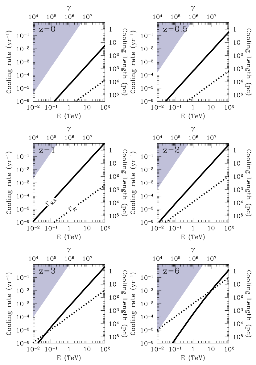
where denotes the Thompson cross section. The strong redshift dependence arises from the rapid increase in the CMB energy density with (). Furthermore, since it is , inverse-Compton cooling is substantially more efficient at higher energies. The associated cooling rate is shown as a function of for a number of redshifts in Figure 2.
When we set , we obtain the following upper limit upon the beam density:
| (7) | ||||
Where we have defined to be the isotropic-equivalent luminosity (per unit energy) of a source located a distance from the region in question. Setting to a typical value () gives an idea of the typical pair-beam densities. Note that despite the large blazar luminosities we consider, the associated beams are exceedingly dilute, a point that is of critical importance in the following section. Since is independent of , this has no implication for inverse-Compton cooling itself.
3 Cooling Ultra-Relativistic Pair Beams via Plasma Beam Instabilities
Plasma beams are notoriously unstable, with the instabilities driven by the anisotropy of the lepton distribution function. Here we consider the implications of these instabilities upon the ultimate fate of the kinetic energy in the TeV-blazar driven pair beams.
3.1 A Fundamental Limit Upon Plasma Cooling Rates
For collective phenomena to be relevant, it is necessary for many pairs to be present within each wavelength of the unstably growing modes. As we shall see, the relevant scale for the beam plasma instabilities we describe below is the plasma skin depth of the IGM,
| (8) |
where is the IGM plasma frequency and is the IGM free-electron number density. Generally, the growing mode must be uniform on scales considerably larger than , both longitudinally and transversely (otherwise it is not well-represented as a single Fourier component), and thus the volume in which many particles must be present is much larger than that defined by a sphere of diameter . Nevertheless, this gives us a conservative constraint, i.e., we require
| (9) |
With Equation (5) this gives a maximum plasma cooling rate:
| (10) |
Plasma processes with cooling rates that exceed this limit necessarily saturate near this cooling rate. Such a super-critical process can potentially operate only until the beam density is driven below the value at which pairs can support collective phenomena, at which point they necessarily quench. However, after plasma cooling ceases, the plasma beam density rises again (since is always less than in practice), and thus the super-critical plasma cooling may resume. Since the efficiency of the plasma cooling decreases smoothly to zero at the critical density, this sequence stabilizes near . The associated excluded region is shown by the grey region in the upper-left corner of Figure 2.
The upper limit upon obtained in Equation (7) implies an analogous limit upon the relevant source isotropic-equivalent luminosities. Again, this arises from requiring a sufficient number of beam pairs to be present to support plasma processes. Since the beam density is linearly dependent upon the source luminosity, this gives a constraint upon the latter:
| (11) |
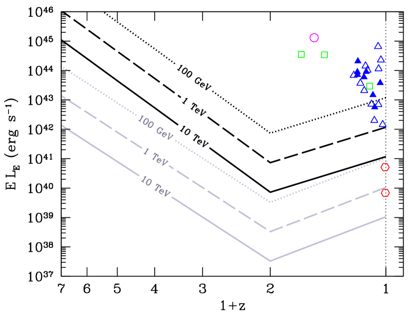
effectively defining a luminosity cut-off, below which collective plasma phenomena may be ignored. This limiting luminosity shown as a function redshift by the grey lines in Figure 3 for various gamma-ray energies. While the luminosity limit does depend upon , it is clear that all of the observed TeV blazars (listed in Table 1) are sufficiently luminous for their resulting pair beams to support collective phenomena at the redshifts of interest for active galactic nuclei (AGNs). The only source to fall marginally below the limiting luminosity at is the radio galaxy Cen A (the lower-most point in Figure 3), the closest and dimmest object in Table 1.
3.2 Cold Plasma Beam Instabilities
Within astrophysical contexts there are at least two well known beam instabilities: two-stream and Weibel, the latter having been suggested as a mechanism for magnetizing strong shocks (Medvedev & Loeb, 1999), and both implicated in the coupling at collisionless shocks (Spitkovsky, 2008). These are, however, simply different limiting examples of the same underlying filamentary instability, for which the maximum growth rate exceeds either – the so-called “oblique” mode, which we discuss below (Bret et al., 2004, 2005a; Lemoine & Pelletier, 2010). Note that since the pair beam is neutral, it contains its own return current and thus beam instabilities that arise due to the electron return currents within the background plasma (e.g., the Bell and Buneman instabilities, see Bret, 2009) are not relevant.
Here we discuss the nature of these instabilities, and their growth rates in the cold-plasma limit (i.e., mono-energetic beams). While the low-temperature approximation is unlikely to be applicable in practice for the beams of interest here, it provides a convenient limit in which to present the relevant processes within their broader context. For a similar reason, and because we have not found analogous derivations elsewhere in the astrophysical literature, we present the ultra-relativistic pair beam instability growth rates for the two-stream and Weibel instabilities in Appendixes A.1 and A.2, only summarizing the results here. We defer a discussion of the more directly relevant warm-plasma oblique instability to the following section. Generally, we find that the plasma instabilities are capable of dominating inverse Compton cooling as a means to dissipate the bulk kinetic energy of the pair beams from TeV blazars.
The pair two-stream instability arises due to the interaction of the anisotropic electron and positron distribution functions with the comoving background electrostatic wave (i.e., , where is the electromagnetic mode wavevector and is the beam momentum) with wavelength for , which is generally the case of interest here. The associated cooling rate999Note that since we are interested in the rate at which energy is lost, these are necessarily twice the instability “growth” rates, defined by the e-folding time of the electromagnetic wave amplitudes. in the cold-plasma limit is
| (12) |
which depends only weakly upon the IGM density and the pair beam density, though decreases rapidly as becomes large.
The Weibel instability is associated with coupling to a secularly growing, anharmonic transverse magnetic perturbation (i.e., ). The most rapidly growing wavelength is again that associated with the background plasma skin depth, , with associated cooling rate in the cold-plasma limit
| (13) |
which depends only upon the pair beam density and the pair Lorentz factor. At large this is suppressed more weakly than the two-stream instability, though is a moderately stronger function of .
The computation of the growth rates of the two-stream and Weibel instabilities are greatly simplified by the particular geometries of the coupled electromagnetic waves and beam momenta. However, a generalized oblique treatment has shown the presence of continuum of unstable modes (Bret et al., 2004, 2005a; Bret, 2009; Bret et al., 2010b; Lemoine & Pelletier, 2010), characterized by the orientation of their wave-vector relative to the bulk beam velocity. Of these neither the two-stream nor Weibel are generally the most unstable. Rather, generically the most robust and fastest growing mode occurs at oblique wave-vectors, and thus referred to as the oblique instability by Bret et al. (2010b). The cold-plasma cooling rate of this maximally-growing mode is
| (14) |
This can be much larger than the two-stream and Weibel growth rates when and .
3.3 Warm Plasma Beam Instabilities
The cold-plasma oblique instability cooling rates dominate inverse-Compton cooling by orders of magnitude over the region of interest. However, at the very dilute beam densities of relevance here, the cold-plasma approximation requires exceedingly small beam temperatures. Above an IGM-frame temperature of roughly
| (15) | ||||
pairs can traverse many wavelengths of the unstable modes over the cold-instability growth timescale, a situation commonly referred to as the kinetic regime. As a consequence, significant phase mixing can occur, substantially reducing the effective growth rate (Bret et al., 2010a).
The way in which finite beam temperatures limit the growth rate depends sensitively upon the nature of the velocity dispersion and the modes of interest (see, e.g., Bret et al., 2005b). For example, the two-stream instability, associated with wave vectors parallel to the beam, enters the strongly suppressed “quasi-linear” regime when the parallel momentum dispersion is large, though is insensitive to even large transverse dispersions. Conversely, the Weibel instability, associated with wave vectors orthogonal to the beam, is sensitive to even small transverse velocity dispersions but unaffected by large parallel velocity dispersions. This is simply because a given mode can tolerate large velocity dispersions within but not across the phase fronts of the unstable electromagnetic modes. For the situation of interest here, dilute beams and cool IGM (i.e., ), the oblique modes are nearly transverse, and thus sensitive primarily to large transverse velocity dispersions.
Nevertheless, even for the small temperatures we have inferred for the pair beams, we find ourselves in the kinetic regime. In this case the oblique instability cooling rate has been numerically measured to be
| (16) |
where we have set the beam temperature in the beam frame to , and thus (Bret et al., 2010a). Both the cold and hot growth rates have been verified explicitly using particle-in-cell (PIC) simulations, though for somewhat less dilute beams than those we discuss here (Bret et al., 2010b).
When the kinetic oblique mode dominates the beam cooling the beam density is given by
| (17) |
The associated cooling rate is then
| (18) |
This is a stronger function of gamma-ray energy than inverse-Compton cooling, implying that it will eventually dominate at sufficiently high energies, assuming a flat TeV spectrum. In addition it is a very weak function of , being only marginally faster in lower-density regions, and thus the cooling of the pairs is largely independent of the properties of the background IGM.
The rates obtained by numerically solving Equation (5) for , with , are shown for a number of redshifts in Figure 2. For the luminosity shown (, typical of the bright TeV blazars) at plasma cooling dominates inverse Compton above a TeV. In the present epoch, is roughly two orders of magnitude larger than for bright TeV blazars.
The luminosity dependence of implies a luminosity limit below which inverse Compton does dominate the linear evolution of the pair beam,
| (19) |
(note that at this luminosity , and thus
is half the value shown in Equation (17)).
This limit is shown as a function of redshift for a number of different
energies by the black lines in Figure 3. Note that
these lie above the corresponding limits associated with the
applicability of the plasma prescription, suggesting that in practice
the beam does support collective phenomena. The critical luminosity
ranges from to ,
depending upon redshift and energy of interest. It also depends
upon the over-density as roughly , and thus
at low densities the critical luminosity is moderately smaller.
The only two sources in Table 1 which fall below
the plasma-cooling luminosity limit are the radio galaxies M87 and Cen
A, both of which are detectable only as a result of their close
proximity. At , all but a handful of the remaining
sources lie more than an order of magnitude above this limit, and in
the case of the two sources that dominate the TeV flux at Earth,
more than two orders of magnitude above this limit.
3.4 Intuitive Picture of the two-stream, Weibel, and Oblique Instabilities
Given the technical nature of our discussion above, it is useful to have a qualitative understanding of these instabilities. We caution, however, that intuitive pictures of plasma processes frequently fail to capture all the relevant physics. Hence, generalization of these intuitive pictures beyond their limited range of applicability is potentially misleading. This is explicitly illustrated by our examples here: all of the instabilities discussed in this work belong to the same family, i.e., instabilities that arise from interpenetrating plasmas, but the underlying qualitative pictures for each differ substantially.
We begin with the Weibel (or filamentation) instability (Weibel, 1959), for which a mechanical viewpoint (an initial magnetic perturbation deflects particles into opposing current streams that reinforce the perturbed field) can be found in Medvedev & Loeb (1999), to which we refer the interested reader. Here we present picture that although having the virtue of being simpler is not entirely correct: because like currents attract, small-scale current perturbations arising out of the fluctuations within the interpenetrating plasmas will coalesce preferentially to produce increasingly larger-scale currents. These induce stronger magnetic fields, and thus larger attractive Lorentz forces between neighboring currents; a positive feedback loop develops leading to instability. This process continues until the associated magnetic field strengths become sufficiently large to disrupt the currents (in the case of equal density beams) or until the transverse velocity of the constituent particles is large enough to efficiently migrate between current structures on the linear growth timescale, i.e., enter the kinetic regime.
We should note that the aggregation of currents in the Weibel instability does not rely upon oscillatory waves.101010The linear analysis of the Weibel instability assumes wave-like disturbances in the plasma. However, there is no associated restoring force to these waves and, hence, they do not oscillate. Hence, there is no oscillatory component to this instability – it is a purely growing mode. In contrast, the two-stream instability is an overstable mode, where the oscillatory components are Langmuir (or plasma) waves with a wavevector parallel to the beam velocity. These are longitudinal waves, associated with local charge oscillations, and are completely described by a propagating perturbation in the electrical potential. As particles in the beam traverse Langmuir waves in the background plasma, they experience successive periods of acceleration and deceleration, with electrons (positrons) collecting in minima (maxima) of the electric potential, where the particle speeds are at their smallest.111111One tempting aspect is to think of these particles as almost massless and hence imagining that these electric fields are quickly shorted out. While this is the case in most astrophysical process, we urge the reader to resist this temptation because these instabilities occur on short enough timescales that the mass of these charged particles plays a crucial role in the physics of the instability. This charge-separated bunching of the beam plasma enhances the background electric perturbation, potentially growing the background Langmuir wave.
The bunching within the beam is simply an excitation of Langmuir waves within the beam plasma itself. Thus the growth of the charge perturbations in the background and beam plasmas corresponds to the resonant coupling between Langmuir waves in the background and beam. When the beam density is much less than the background density, as is the case here, background and beam Langmuir waves only overlap in frequency, and therefore satisfy the conditions for resonance, when the wavevector of the latter is parallel to the beam velocity (see the discussion above Equation (43)). This is always satisfied for the family of comoving beam Langmuir waves (i.e., waves which in the beam frame move counter to the background plasma). However, of particular importance for the two-stream instability are the counter-propagating beam Langmuir waves (i.e., waves which in the beam frame move parallel to the background plasma). If the beam velocity exceeds the phase velocity of these waves (as seen in the beam frame), the counter-propagating wave will be dragged in the direction of the beam (as seen in the background frame), and therefore has a wavevector which satisfies the resonant condition.
Nevertheless, the counter-propagating Langmuir wave still carries momentum in the direction opposite to the beam. Thus, as the counter-propagating wave grows, the momentum, and therefore energy, of the beam-wave system necessarily decreases. This implies that the counter-propagating Langmuir wave is also a negative energy mode as seen in the background frame. As a consequence, the resonant coupling can transfer energy to the positive-energy background wave from the negative-energy beam wave, while growing the amplitudes of both, and thereby leading to instability. Note that if the phase velocity of the counter-propagating Langmuir wave is larger than the beam velocity, it no longer is dragged in the direction of the beam and no longer satisfies the necessary resonant condition. For a distribution of particles, this constraint upon the velocities within the beam corresponds to the familiar Penrose criterion (Sturrock, 1994; Boyd & Sanderson, 2003), and is satisfied in the pair beams resulting from VHEGRs.
The oblique instability encompasses the two-stream and Weibel instabilities, though the most unstable mode is most similar to the former in that the intuitive picture focus solely on the electrostatic forces, ignoring electromagnetic forces.121212The picture we present here for the oblique instability is discussed in Nakar et al. (2011). In practice, this is a relatively good approximation and can be used to calculate the growth of these modes in idealized situations (e.g. Nakar et al., 2011; Bret et al., 2004). The qualitative picture proceeds similarly to that for the two-stream instability described above, with the minor modification that the perturbing background Langmuir waves now move at an angle relative to the relativistic beam. As a consequence, the resonant Langmuir waves have a phase velocity such that . From the simple intuitive picture above, if is selected such that the projected beam velocity is slightly faster than the nearly resonant Langmuir wave, an instability develops.
Finally, to understand why the growth rates between the two-stream instability above and the oblique instability differ, it is useful to make the approximation that the electric fields generated are in the direction of the k-vector. In the two-stream case, the electric field must slow down (or speed up) particles. This gets progressively harder for more relativistic particles. In the oblique case, the electric field deflects the particles, changing their projected velocity. While this is also more difficult for more relativistic particles, this is not nearly as hard as changing the particles parallel (along the beam) velocity. Hence, the oblique instability more easily drives charge density enhancements (and therefore instabilities) at large , i.e., easier deflection, than the two-stream instability.
3.5 Non-Linear Saturation
We have thus far only treated the linear development of the relativistic two-stream, Weibel, and oblique instabilities. However, the impact pair beams have upon the IGM, gamma-ray cascade emission, and measures of the IGMF will ultimately depend upon their nonlinear development. To address this, however, we are presently forced to appeal to analytical and numerical calculations of systems in somewhat different (and less extreme) parameter regimes.
Motivated by the applicability of the Weibel instability in the context of GRBs, the nonlinear saturation of the relativistic Weibel instability for equal density plasma beams is well understood analytically and numerically. Initially, the Weibel instability rapidly grows until the energy density of the generated magnetic field becomes of order the kinetic energy of the two beams (Silva et al., 2003; Frederiksen et al., 2004; Chang et al., 2008). Analytically, Davidson et al. (1972) argued that the Weibel instability would saturate when the generated magnetic fields become so large that the Larmor radius of the beam particles is of order the skin depth, i.e., when the energy of generated magnetic fields is equal to the kinetic energy of two equal density relativistic beams (see also Medvedev & Loeb, 1999). The particles rapidly isotropize with a Maxwellian distribution (Spitkovsky, 2008), i.e., heat, and the magnetic energy then rapidly decays within an order of a few tens of skin depths (Chang et al., 2008). Hence for two equal density, relativistic, interpenetrating beams, the Weibel instability converts anisotropic kinetic energy into heat. However, as we have already noted, for the pair beams of interest here the Weibel instability is completely suppressed for tiny transverse beam temperatures. Hence, while this instability may initially operate, it may quickly become suppressed if it results in significant transverse heating of the beam.
Unlike the Weibel instability, the two-stream and kinetic oblique instabilities continue to operate, though more slowly than implied by their cold-plasma limits, in the presence of substantial beam temperatures. Due to the geometry of the coupled modes, the oblique instability is primarily sensitive to transverse beam-velocity dispersions, though shares the resistance to beam heating with its two-stream cousin (Bret et al., 2005b; Bret, 2009; Bret et al., 2010b; Lemoine & Pelletier, 2010). Unlike the two-stream instability, the oblique instability in the parameter range of interest here is also largely insensitive to longitudinal heating. Thus, generally, it appears that the oblique instability is substantially more robust than its more commonly discussed brethren.
What is less clear a priori is if these instabilities primarily heat the beam or primarily heat the background plasma. Here we appeal to the numerical simulations of Bret et al. (2010b), where a mildly relativistic beam () penetrating into a hot, dense background plasma (beam-to-background density ratio of ) was studied. In these the oblique instability resulted in a significant fraction () of the beam energy heating the background plasma before the heating of the beam suppressed the oblique instability in favor of the two-stream instability. The relative effectiveness with which the beam heats the background plasma is due to the efficiency with which the longitudinal electrostatic modes are dissipated in the background plasma; unlike electromagnetic modes (e.g., those generated by the Weibel instability), electrostatic modes are rapidly dissipated via Landau damping.
We note that Bret et al. (2010b) found that the heating of the beam by the oblique instability eventually led to its suppression, allowing the two-stream instability to grow, continuing the dissipation of the beam kinetic energy. As a result, in their simulations a total of 30% of the energy was deposited into the background plasma via a combination of the oblique and two-stream instabilities, i.e., an additional 10% of the beam energy was thermalized via the two-stream instability during and after the suppression of the oblique instability.
In our case, we expect that much more beam energy (more than the 20%, and possibly up to ) will be deposited into the background IGM because we are much deeper into the regime in which the oblique instability dominates, i.e., and . In particular, for the case of interest here, and
| (20) |
The extremely large Lorentz factor and tiny density ratio make it computationally prohibitive to assess the beam evolution with numerical PIC directly. Nevertheless, because we find ourselves in a regime in which the oblique instability is much more strongly dominant than that simulated in Bret et al. (2010b), we expect the linear growth of the kinetic oblique instability to continue for much longer before the beam changes character and moves out of the oblique-dominated regime — potentially once of the beam energy has been dissipated. However, this remains to be studied in future work.
The effect of nonlinear processes might also effect the evolution of the linear instability. For instance, Lesch & Schlickeiser (1987) argued that for the relativistic electrostatic two-stream instability, nonlinear coupling to daughter modes arrest the growth of the linearly unstable mode at a very low mode energy. Hence, they claim that the electrostatic two-stream instability can only bleed energy from the beam at a slow rate.
Utilizing the order of magnitude estimates in Lesch & Schlickeiser (1987) or the expression for nonlinear Landau damping in Melrose (1980), we have found that damping of the pair beam via the relativistic two-stream instability could be highly suppressed. The oblique instability may be similarly suppressed, however, this effect is much more marginal due to the instabilities much larger growth rate. Nevertheless, determining its behavior for the parameters relevant here is an important unanswered question that is left for future work. For the purposes of this paper, we will rely upon the intuition developed from numerical studies of the oblique instability and argue that the beam ends up heating the IGM primarily.
In what follows, we will presume the nonlinear evolution of the “oblique”
or related plasma instabilities lead to the heating of the background IGM,
i.e., beam cooling. However, we note that the beam itself may
be the primary recipient of this kinetic energy, i.e., beam disruption. Most
of our results depend critically on beam cooling and not beam disruption. This includes
the effect of blazar heating on the IGM temperature-density relation studied in Paper II, the effects
on structure formation studied in Paper III, the excellent
reproduction of the statistical properties of the high-redshift Ly forest found in Puchwein et al. (2011),
and the implications on the EGRB and the
redshift evolution of TeV blazars studied in Section 5. However, our conclusions
on the inapplicability of IGMF constraints determined from the non-observation
of GeV emission from blazars still remains in the presence of beam disruption.
This is because the self-scattering of pairs in the beam would
suppress this GeV emission in similar manner to an IGMF.
3.6 Suppression of the Oblique Instability by an IGMF
The beam instabilities we have discussed have been analyzed primarily within the context of unmagnetized plasmas. However, for a variety of theoretical reasons a weak IGMF is not unexpected. For example, a field strength of is sufficient to explain the observed galactic fields via compression and winding alone. Here we consider the implications that an IGMF has for the instability growth rates we have described above.
A strong IGMF causes the ultra-relativistic pairs to gyrate, and therefore to isotropize, suppressing the growth of instabilities that feed upon the beam anisotropy (e.g., those we have described above). However, for this to efficiently quench the growth of the plasma beam instabilities, this isotropization must occur on a timescale comparable to the instability growth time, i.e., the Larmor frequency must be comparable to the cooling rate, . This condition gives a lower-limit upon IGMF strengths sufficient to appreciably suppress the growth of plasma beam instabilities of
| (21) |
considerably larger than those typical of both, primordial formation mechanisms (Widrow, 2002) and implied by galactic magnetic field estimates, assuming galactic fields are produced by contraction and winding alone.
Because the VHEGRs emitted by the TeV blazars travel cosmological distances prior to producing pairs, an IGMF capable of suppressing the plasma beam instabilities must necessarily have a volume filling fraction close to unity. In particular, it must permeate the low-density regions, where most of the cooling occurs. However, the Alfvén velocity within those areas is extraordinarily small, roughly
| (22) |
The IGM sound speed,
| (23) |
is considerably larger, implying convection is much more efficient. Nevertheless, even after substantial heating via the thermalization of the TeV blazar emission (Paper II) is taken into account, magnetic fields will have propagated over a Hubble time via convection and much less via diffusion, implying that a pervasive, sufficiently strong magnetic field can not be produced via ejection from galactic dynamos. While galactic winds can produce much faster outflows, , unless they inject a mass comparable to that contained in the low-density regions over a Hubble time, they are rapidly slowed via dissipation at shocks in the IGM, again limiting the spread of galactic fields. Moreover, we note that since the magnetic field must be volume filling to suppress the plasma beam cooling substantially it is insufficient to produce pockets of strong fields, and thus any galactic origin powered by winds requires a nearly complete reprocessing of the low-density regions. However, the ultimate thermalization of such fast, dense winds would raise the IGM temperature to , in conflict with the Ly forest data and exceeding the entire bolometric output of quasars by at least a factor of two. For these reasons we conclude that a volume-filling strong IGMF would demand a primordial origin.
4 Implications for IGM Magnetic Field Estimates
The existence of plasma processes that can cool the pair beams associated with TeV blazars has profound consequences for efforts to constrain the IGMF using the spectra of TeV blazars. Here we describe how the reported IGMF limits have been obtained, the consequences of plasma cooling for these, and potential strategies for overcoming the constraints it imposes.
The general argument made in efforts to constrain the IGMF based upon the GeV emission from blazars proceeds as follows: The beamed TeV blazar emission pair-creates off of the EBL. The resulting pairs subsequently up-scatter CMB photons to GeV energies. In principle, this should produce an observable GeV excess, or bump, in the spectra of these objects. However, in the presence of a large-scale IGMF, the ultra-relativistic pairs can be deflected significantly, directing the beamed GeV emission away from Earth. Thus, it is argued, the lack of a discernible GeV bump in a number of TeV blazars implies a lower limit upon the IGM field strength (as a function of TeV jet opening angle and variability timescale). The crucial components of the argument are
-
1.
The TeV emission is beamed with the typical opening angles inferred from radio observations of AGN jets.
-
2.
The variability timescale within the TeV source is long in comparison to the geometric time delays between the original TeV and inverse-Compton produced GeV gamma rays due to the orbit of the pairs through some angle , (see Dermer et al., 2011).
-
3.
The pairs produced by TeV absorption on the EBL cool primarily via inverse-Compton scattering the CMB (and therefore evolve only due to inverse-Compton cooling and orbiting within the large-scale IGMF).
The first of these is supported indirectly by the lack of TeV emission from non-blazars. The implied TeV source stability required by the second is at odds with the variability observed in blazars at longer wavelengths. However, since the TeV-GeV delay is a strong function of deflection angle, given an empirical limit upon the TeV blazar variability timescale (presently , Dermer et al., 2011) it is possible to produce a substantially weaker constraint upon the IGMF () (Dermer et al., 2011; Taylor et al., 2011; Takahashi et al., 2012).
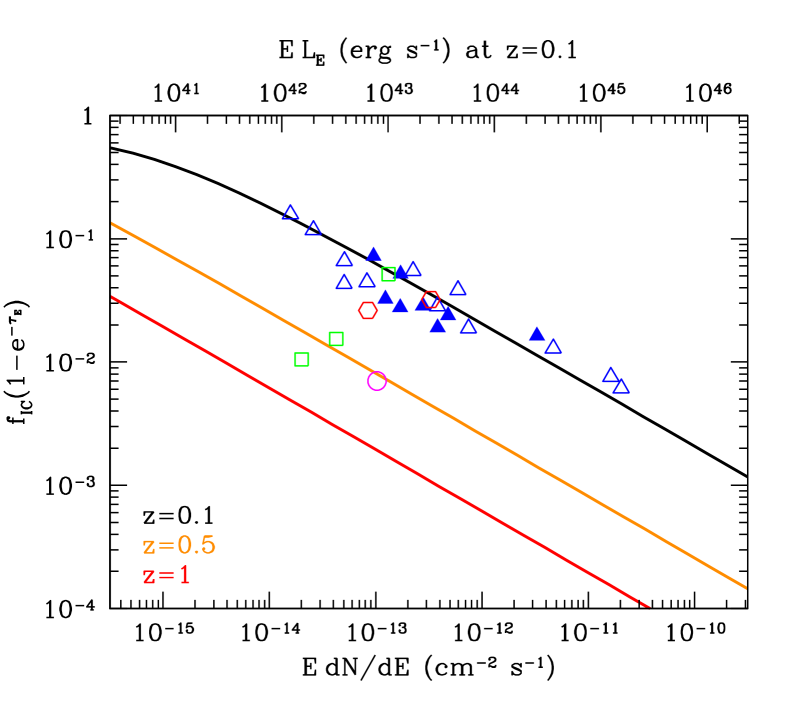
Plasma cooling provides a fundamental limitation for these methods, however, by violating the third condition explicitly. Figures 3 and 4 imply that for all but the dimmest and highest-redshift () gamma-ray blazars only a small fraction of the pair energy is lost to inverse-Compton on the CMB ().131313Here we implicitly assume that the nonlinear saturation of the plasma instabilities extract energy from the pair beam at the linear growth rate. In particular, the black lines in Figure 3 shows where , i.e., roughly 50% of the TeV-photon power is ultimately converted into heat via plasma instabilities. As a result, the putative GeV component is typically much less luminous than otherwise expected, reducing the significance of non-detections substantially.
This may be seen explicitly in Figure 4, which shows as a function of gamma-ray flux for (corresponding to a Comptonized-CMB photon energy of approximately ), at number of source redshifts. Typical values for the TeV blazars collected in Table 1 (including those employed by Neronov & Vovk, 2010; Tavecchio et al., 2010, 2011; Dermer et al., 2011; Taylor et al., 2011; Takahashi et al., 2012; Dolag et al., 2011) lie in the range to , implying correspondingly small GeV Comptonization signals.
More importantly, when the beam evolution is dominated by plasma instabilities, over the inverse-Compton cooling timescale the pair distribution necessarily becomes isotropized. As a consequence, the angular distribution of the resulting GeV gamma rays (i.e., the orientation of the GeV “beam”) is no longer indicative of the beam propagation through a large-scale magnetic field. That is, one expects large-angle deviations regardless of the IGMF strength.
Unfortunately, subject to the caveats of the preceding section, plasma instabilities appear to be the dominant cooling mechanism for the pair beams associated with the TeV blazars that have been used to constrain the IGMF thus far. The isotropic-equivalent luminosities of these sources range from to , placing them well within the plasma-instability dominated regime. As a result, the reported IGMF limits inferred from TeV blazars are presently unreliable.
Nevertheless, it may be possible to avoid the limitations imposed by plasma instabilities. At sufficiently low pair densities the cooling rates associated with the beam instabilities described in Section 3 fall below that due to inverse Compton. Moreover, at some point the plasma prescription breaks down altogether, suggesting that any plasma instabilities that operate on the skin-depth of the IGM are strongly suppressed. There are two distinct ways in which low pair densities can arise: low intrinsic luminosities and very short timescale events.
Below isotropic-equivalent luminosities of roughly inverse-Compton cooling dominates the beam instabilities we describe in Section 3 at . Below the plasma prescription itself breaks down altogether. While no TeV blazars with isotropic-luminosities below are known, there are a handful of very nearby sources below . The two dimmest sources, the radio galaxies M87 and Cen A, however, are observable only due to their proximity (i.e., they have proper distances ), intrinsically preventing them from providing a significant constraint on the IMGF. The highest source in Figure 4, and thus presumably the source with the largest fractional inverse-Compton signal, is PKS 2005-489, a dim, soft TeV blazar at . Even in this case, however, the inverse-Compton cooling timescale is roughly 4 times longer than the plasma cooling timescale. Hence, probing the IGMF with TeV blazars will require observing considerably dimmer objects than those used thus far. Since doing so will likely require substantial increases in detector sensitivities141414As described in Section 5.1.2, the incompleteness of the TeV observations are well-described by a single flux limit, corresponding to an isotropic-equivalent luminosity limit at of roughly . The flux limit of Fermi is estimated to be roughly at (see Figure 23 of Abdo et al., 2010c). we will not consider this possibility any further here.
Low pair densities may also be produced by limiting the duration of the VHEGR emission. Equation (5) was derived assuming that the pairs had reached a steady state between their formation via VHEGRs annihilating upon the EBL and their cooling via inverse-Compton and plasma processes. However, it takes roughly a cooling timescale for the pair beam densities to saturate at this level, which can be as long as at some and . Therefore, generally there is a lag between the onset of the VHEGR emission and the time at which plasma processes begin to dominate the cooling of the beam.
We can estimate this by setting where is the duration of the emission. This is the case when the pair density is initially zero (i.e., it has been many cooling timescales since the last period of VHEGR emission) and . Inserting this into the various cooling rates and setting gives an estimate for the maximum duration for which the pair density remains sufficiently low that inverse-Compton cooling dominates the cooling:
| (24) |
which may be found for the observed TeV sources in Table 1. Typically for the blazars that have been used to constrain the IGM, though ranges from to for TeV blazars generally. Note that it is not sufficient for emission to vary on ; such variations will be temporally smoothed on the much larger cooling timescale. Rather, it is necessary for the source to have been quiescent (i.e. isotropic-equivalent luminosity considerably less than ) for periods long in comparison to and have turned on less than a time ago. As a consequence, only IGMF estimates using new TeV blazars can potentially avoid plasma instabilities in this way.
A natural example of a class of transient gamma-ray sources is gamma-ray bursts (GRBs). For GRBs an isotropic-equivalent energy of roughly is required for the plasma instabilities to grow efficiently, comparable to the total energetic output of the brightest events. Using GRBs to probe the IGMF has been suggested previously, and limits based upon the lack of a delayed GeV component in some GRBs already exist, finding field strengths above (see, e.g., Plaga, 1995; Dai & Lu, 2002; Guetta & Granot, 2003; Takahashi et al., 2008). Future efforts should be able to probe field strengths of for (see Figure 4 of Takahashi et al., 2008). This is predicated, however, upon the existence of a significant VHEGR component in the prompt or afterglow emission of GRBs.
Ando & Kusenko (2010) have attempted to directly detect the GeV signal in the vicinity of AGNs that do not exhibit TeV emission. That is, since an IGMF can in principle induce large-angle deviations in the propagation direction of the up-scattered GeV photon relative to the original VHEGR, one may search for a GeV excess at large distances from non-blazars. This is made much more difficult by the extraordinarily low surface gamma-ray brightness due to the large , random source orientations, and potential dilution associated with the beam diffusion. Nevertheless, Ando & Kusenko (2010) claim a marginal detection of this component in stacked Fermi images, though the Fermi point-spread function appears to be capable of completely explaining their result (Neronov et al., 2011). If such a GeV-halo were found around TeV-bright sources with the anticipated luminosity, it would argue strongly against plasma instabilities dominating the beam evolution. However, we note that for many TeV-dim sources inverse-Compton cooling still dominates the beam evolution, and thus in stacked images of these sources GeV-halos may still be present.
Note that, as discussed in Section 3.6, a strong IGMF () could, in principle, suppress the growth of the plasma beam instabilities significantly. As we argue there, a sufficiently pervasive and strong IGMF would necessarily be primordial in origin. However, few constraints upon such a primordial field exist, especially since we have argued that the lack of an inverse Compton GeV bump cannot be used as a constraint on the IGMF. Hence, we are left with constraints from Big Bang Nucleosynthesis (, Kandus et al., 2011, and references therein), from the CMB (, Barrow et al., 1997), and limits on the Faraday rotation of distance radio sources (, Vallée, 2011, and references therein). A stronger limit can be obtained from limits upon the deflection angle () of ultra-high energy cosmic rays () from distant sources at a distance , which upon assuming a magnetic correlation length, , gives (see for instance Waxman & Miralda-Escude, 1996; de Angelis et al., 2008), though this depends strongly upon the assumed structure of the IGMF and small-scale fields may be significantly stronger than this (Kotera & Lemoine, 2008). Proposed mechanisms by which a primordial IGMF can be theoretically generated are essentially unconstrained, yielding B-field strengths between – (Kandus et al., 2011).
However, in the remainder of this work and in Paper II and Paper III, we show that the effect of the "oblique" (or similar) instability may potentially explain many different observed phenomena in cosmology and high energy astrophysics. Taking the beam instabilities we present here at face value, that so many observational puzzles can be simultaneously explained by the local dissipation of TeV blazar emission would imply the strongest upper limit upon primordial magnetism to date. Namely, the apparent impact of TeV blazars upon the large-scale cosmological environment places a constraint on the IGMF of .
5 Implications for the Blazar Luminosity Function
The EGRB corresponds to the diffuse gamma-ray background () not associated with Galactic sources. This has been measured at high energies by EGRET (Sreekumar et al., 1998; Strong et al., 2004) and more recently strongly constrained between and by Fermi (Abdo et al., 2010b, a). The most recent Fermi estimate of the EGRB is a featureless power-law, somewhat softer than that found by EGRET, and does not exhibit the localized high-energy excess claimed by a reanalysis of the EGRET data (Strong et al., 2004).
While bright, nearby blazars are resolved, and therefore excluded from the EGRB, the remainder is thought to arise nearly exclusively from distant gamma-ray emitting blazars, upon which the Fermi EGRB places severe constraints (Abdo et al., 2010b). Beyond Fermi cannot detect blazars with isotropic-equivalent luminosities comparable to the objects listed in Table 1, and thus the vast majority of such objects contribute to the Fermi EGRB.
A significant EGRB above is not expected due to annihilation upon the EBL. However, if they operate efficiently, ICCs can reprocesses the VHEGR emission of distant sources into the Fermi EGRB energy range (i.e., ). Thus, a number of efforts to constrain the VHEGR emission from extragalactic sources based upon the EGRB can be found in the literature (Narumoto & Totani, 2006; Kneiske & Mannheim, 2008; Inoue & Totani, 2009). These have typically found that the comoving number density of VHEGR-emitting blazars could not have been much higher at high- than it is today. Even with moderate evolutions (e.g., that in Narumoto & Totani, 2006; Inoue & Totani, 2009) consistent with the EGRET EGRB, substantially over-produce the Fermi EGRB, and are therefore believed to be excluded (Venters, 2010).
However, here we show that this conclusion is predicated upon the high-efficiency of the ICC. We have already shown that for bright VHEGR sources plasma beam instabilities extract the kinetic energy of the first generation of pairs much more rapidly than inverse-Compton scattering. As a consequence, the ICC is typically quenched, substantially limiting the contributions of these sources to the EGRB. Thus, even with a dramatically evolving blazar population, e.g., similar to that of quasars, it is possible for these objects to be consistent with the Fermi EGRB. While our discussion of the EGRB and the evolution of blazars is predicated on the extraction of the pair-beam kinetic energy by plasma beam instabilities, our conclusions are not. Rather they will continue to hold as long as the pair beams are locally dissipated – via plasma beam instabilities or some other equally powerful mechanism.
5.1 An Empirical Estimate of the TeV Blazar Luminosity Function
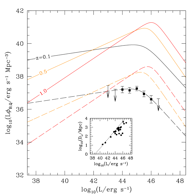
Blazars dominate the extragalactic gamma-ray sky, and thus represent the best studied VHEGR source class. Since we are interested exclusively in those objects responsible for the bulk of the VHEGR emission, we necessarily concentrate upon the subset of blazars that are luminous VHEGR emitters. Of the 28 TeV sources listed in Table 1, 23 are peaked at very-high energies (the HBL and hard IBL sources, for a full definition see below), and comprise what we will call collectively TeV blazars. This necessarily is limited to as a consequence of the annihilation of VHEGRs upon the EBL. Nevertheless, we will find that this is remarkably similar to the local quasar luminosity function (), and thus attempt to construct a blazar luminosity function by analogy:
| (25) |
in which is the comoving number density of blazars at redshifts less than with isotropic-equivalent luminosities below . This is different from previous efforts to empirically constrain from the EGRB (see, e.g., Narumoto & Totani, 2006; Inoue & Totani, 2009) in at least two ways. First, we begin with an empirically determined local and attempt to extend this by placing the TeV blazars within the broader context of accreting supermassive black holes, rather than beginning with the EGRB and working backwards to infer an acceptable . Second, we are primarily concerned with of TeV blazars, and specifically do not consider the contributions from other kinds of objects. While this does not represent a significant oversight in terms of the high-energy contributions to the EGRB, which almost certainly arises from the VHEGR-emitting blazars, it does mean that our conclusions regarding the luminosity function of the TeV blazars do not necessarily apply to all Fermi AGN (e.g., the FSRQs, see below).
5.1.1 Placing TeV blazars in Context
The TeV blazars presumably fit within the broader context of the blazars observed by Fermi specifically, and AGNs generally. For this reason, here we briefly review the physical classification scheme based on the widely accepted AGN standard paradigm that provides a unified picture of the emission emission properties of these objects (e.g., Urry & Padovani, 1995). Specifically, we summarize the classes of objects believed to be capable of producing significant TeV luminosities and the potential physical processes responsible for the observed emission. Based upon these we then assess the implications for the number, variability, and redshift evolution of the TeV blazars.
In general there exist two main classes of AGNs that differ in their accretion mode and in the physical processes that dominate the emission.
-
1.
Thermal/disk-dominated AGNs: Infalling matter assembles in a thin disk and radiates thermal emission with a range of temperatures. The distributed black-body emission is then Comptonized by a hot corona above the disk that produces power-law X-ray emission. Hence the emission is a measure of the accretion power of the central object. This class of objects are called QSOs or Seyfert galaxies and make up about 90% of AGNs. They preferentially emit in the optical or X-rays and do not show significant nuclear radio emission. None of these sources have so far been unambiguously detected by Fermi or imaging atmospheric Cherenkov telescopes because the Comptonizing electron population is not highly relativistic and emits isotropically, i.e. there is no beaming effect that boosts the emission.
-
2.
Non-thermal/jet-dominated AGNs: The non-thermal emission from the radio to X-ray is synchrotron emission in a magnetic field by highly energetic electrons that have been accelerated in a jet of material ejected from the nucleus at relativistic speed. The same population of electrons can also Compton up-scatter any seed photon population either provided by the synchrotron emission itself or from some other external radiation field such as UV radiation from the accretion disk. Hence the SED of these objects shows two distinct peaks. The luminosity of these non-thermal emission components probes the jet power of these objects. Observationally, this leads to the class of radio-loud AGNs which can furthermore be subdivided into blazars and non-aligned non-thermal dominated AGNs depending on the orientation of their jets with respect to the line of sight.
There are no known sources above that correspond to AGNs with jets pointed at large angles (, see Urry & Padovani 1995) with respect to the line of sight (for an example of a non-aligned AGN, NGC1275, that shows a very steep high-energy spectrum, emitting a negligible number of VHEGRs, see Mariotti & MAGIC Collaboration, 2010). Hence we turn our attention to blazars, which can be powerful TeV sources.
Blazars can further be subdivided into two main subclasses depending upon their optical spectral properties: flat spectrum radio quasars (FSRQ) and BL Lacs. FSRQs, defined by broad optical emission lines, have SEDs that peak at energies below , implying a maximum particle energy within the jet and limiting the inverse-Compton scattered photons mostly to the soft gamma-ray band. It is presumably for this reason that no continuous TeV component has been detected in an FSRQ (note, however, that TeV flares from FSRQs have been detected in two cases (MAGIC Collaboration et al., 2008b; Mose Mariotti, 2010)).
In contrast, BL Lacs or Blazars of the BL Lac type (Massaro et al., 2009) can be copious TeV emitters. These are very compact radio sources and have a broadband SED similar to that of strong lined blazars, though lack the broad emission lines that define those. Depending upon the peak energy in the synchrotron spectrum, which approximately reflects the maximum particle energy within the jet, they are classified as low-, intermediate-, or high-energy peaked BL Lacs, respectively called LBL, IBL, and HBL (Padovani & Giommi, 1995; Abdo et al., 2010d).151515The source classes of HSP/ISP/LSP used in recent Fermi publications are very similar to the commonly used HBL/IBL/LBL classes. Hence we identify these with each other, respectively, though minor differences may be found in the literature. Nevertheless, where we refer to the number counts observed by Fermi specifically, we will refer to the classes HSP/ISP/LSP in keeping with their notation. While LBLs peak in the far-IR or IR band, they exhibit a flat or inverted X-ray spectrum due to the dominance of the inverse-Compton component (see Fig 15 of Abdo et al., 2010d, for a visualization of the SED of BL Lacs). The synchrotron component of IBLs peaks in the optical which moves their inverse-Compton peak into the gamma-ray band of Fermi. HBLs are much more powerful particle accelerators, with the synchrotron peak reaching into the UV or, in some cases, the soft X-ray bands. The inverse-Compton peak can then reach TeV energies (Ghisellini & Tavecchio, 2008; Tavecchio & Ghisellini, 2008; Abdo et al., 2010d).161616For the highest energies scattering occurs in the Klein-Nishina regime, which results in steeper inverse-Compton spectra.
In the gamma-ray band, the subclass of IBLs that emit VHEGRs are almost indistinguishable from the HBLs, suggesting that the location of the synchrotron peak does not uniquely characterize the VHEGR emission from these sources (e.g., due to variations among individual blazars in the magnetic field strength within the synchrotron emitting region and the origins and properties of the seed photons that are ultimately Comptonized). Hence we identify HBLs and VHEGR-emitting IBLs with the single source class of TeV blazars. We note that there is presently no evidence for the hypothetical class of ultra-HBLs that were proposed to have a very energetic synchrotron component extending to -rays (Ghisellini, 1999). If such a population of bright and numerous sources exists, Fermi should have seen it (Abdo et al., 2010c). The ultra-HBLs may have escaped detection from Fermi thus far by being either intrinsically dim -ray sources or very rare objects (Costamante et al., 2007).
TeV blazars have a redshift distribution that is peaked at low redshifts extending only up to . This is most likely entirely a flux selection effect; TeV blazars are intrinsically less luminous than LBLs and FSRQs, with an observed isotropic-equivalent luminosity range of , with the highest redshift TeV blazars also being among the most luminous objects (see Figures 23 and 24 in Abdo et al., 2010c). That TeV blazars should be intrinsically less luminous than FSRQs is not entirely unexpected, however. Ghisellini et al. (2009) have argued that the physical distinction between FSRQs and TeV blazars has its origin in the the different accretion regimes of the two classes of objects. Using the gamma-ray luminosity as a proxy for the bolometric luminosity, the boundary between the two subclasses of blazars can be associated with the accretion rate threshold (nearly 1% of the Eddington rate) separating optically thick accretion disks with nearly Eddington accretion rates from radiatively inefficient accretion flows. The spectral separation in hard (BL Lacs) and soft (FSRQs) objects then results from the different radiative cooling suffered by the relativistic electrons in jets propagating into different surrounding media (Ghisellini et al., 2009). Hence in this model, TeV blazars cannot reach higher luminosities than approximately since they are limited by the nature of inefficient accretion flows that power these jets and by the maximum black hole mass, .
5.1.2 An Empirical Local (z,L)
While we have attempted to place the observed TeV blazars, which we have identified with the HBLs and VHEGR-emitting IBLs, into the broader context of AGNs using the unified model, due to the substantial distinctions in accretion rate, emission properties, object morphology and geometry, it is not obvious that any of the properties of TeV blazars should be similar to those of AGNs more generally. Nevertheless, evidence for a simple connection between the two populations can be found in the similarity between their the luminosity functions (a fact we will exploit later in estimating the redshift evolution of the TeV blazars). Here we define the luminosity for the purposes of defining to be the isotropic-equivalent value associated with emission between and . While this may be considered to be a VHEGR luminosity, because most TeV blazars are peaked within this band, this corresponds to the majority of the emission from these sources.
The objects listed in Table 1 were chosen because they have well defined SEDs, based upon a combination of VERITAS, H.E.S.S., and MAGIC observations. These 28 sources have VHEGR spectra that are well fit by the form,
| (26) |
where is the normalization in units of . The gamma-ray energy flux is trivially related to by , from which we obtain a VHEGR flux,
| (27) |
and for sources with a measured redshift a corresponding isotropic-equivalent luminosity, , where is the luminosity distance.171717Since the VHEGR spectra of TeV blazars typically are peaked above , this overestimates the luminosity by a factor of order unity. The resulting , , , , and are collected in Table 1. In addition we list the redshift, inferred comoving distance, and absorption-corrected intrinsic spectral index, defined at , obtained via
| (28) |
For high-redshift sources can be substantially less than , implying that an intrinsic spectral upper-cutoff must exist.
To produce , we must account for a variety of selection effects inherent in the sample listed in Table 1. The objects in Table 1 were originally selected for study for a variety of source-specific reasons, e.g., existing well known sources, extremely high X-ray to radio flux ratio in the Sedentary High energy peaked BL Lac catalog, hard spectrum sources in the Fermi point source catalog, and flagged as promising by the Fermi-LAT collaboration. In addition, the source selection suffered from the usual problems associated with surveys (e.g., scheduling conflicts with other targets, moon, bad weather, etc.). As a consequence, this sample is somewhat inhomogeneous. Nevertheless, in lieu of a less-biased sample, we will treat it as homogeneous and correct for the selection effects were possible, focusing upon those due to the sky coverage and duty cycle of TeV observations, and those due to sensitivity limits of current imaging atmospheric Cerenkov telescopes.
To estimate the sky completeness and duty cycle of this set of objects we rely upon the all-sky gamma-ray observations of HBL and IBL sources by Fermi (Abdo et al., 2010c). Outside of the Galactic plane, Fermi observes 118 high-synchrotron peaked (HSP) blazars and a total of 46 intermediate-synchrotron peaked (ISP) blazars. Roughly half of the latter are likely to emit VHEGRs as indicated by their flat spectral index between 0.1 and 100 GeV (; see the spectral index distribution of Figure 14 in Abdo et al. (2009)). Of these potential 141 TeV blazars, only 22 have also been coincidentally identified as TeV sources, whereas there are a total of 33 known TeV blazars (29 HBL, 4 IBL). If these 141 sources are all emitters, but have not been detected due to incomplete sky coverage of current TeV instruments, then the selection factor is . In addition, the duty cycle of coincident and emission is .181818Note that we implicitly assume that the luminosity distribution of observed TeV sources reflects the true distribution after accounting for flux incompleteness, and thus constant correction factors (independent of luminosity) can be used to estimate the true distribution. We show that this assumption is fulfilled in Figure 5. Finally, by excluding the Galactic plane for galactic latitudes , this is an underestimate by roughly .
We make a rough attempt to correct for the sensitivity limit of the TeV instruments, inferring a flux limit by fitting the upper-envelope of the TeV-blazar flux–luminosity distance distribution. Somewhat surprisingly, despite the heterogeneous nature of the TeV observations, are remarkably well described by a single flux limit: . This process and the associated limit are shown explicitly in the inset of Figure 5. From this we obtain a maximum redshift, and therefore comoving volume, associated with each luminosity. We then construct by counting the number of TeV blazars per unit in each logarithmic luminosity bin and dividing by the comoving volume. The resulting , weighted by luminosity (and therefore showing the luminosity density in comoving units), is shown in Figure 5. It peaks at , implying that, as expected, these objects are systematically dimmer than most other AGN, and exhibits the broken-power law shape typical of AGN luminosity functions. More importantly, despite a handful of sources with redshifts , the objects in Table 1 are all nearby, and therefore our corresponds to that in the local Universe, i.e., . Based upon this, the inferred present-day TeV-blazar luminosity density is roughly .
Also shown in Figure 5 is the obtained by Hopkins et al. (2007). After rescaling to lower luminosities () and lower luminosity densities (), it provides a remarkably good fit to our (reduced- of 0.13 with 3 degrees of freedom), i.e., we find
| (29) |
where an explicit expression for is given in Appendix B. While there is considerable uncertainty in , especially at low luminosities, it clearly does not fit at higher . This suggests two immediate conclusions:
-
1.
The bolometric output of TeV blazars and quasars are regulated by similar mechanisms, presumably accretion, despite the large difference in luminosity and the details of the emission processes between the two populations.
-
2.
TeV blazars and quasars are contemporaneous elements in a single AGN distribution; specifically, TeV-blazar activity does not lag that of quasars.
5.1.3 Extending to high
Based upon the strong similarities between and , and the associated implications, we make the conservative theoretical assumption that the redshift evolution of the TeV blazars follows that of quasars. That is, we suppose that Equation (29) holds at all . This implies that the integrated comoving TeV-blazar isotropic-equivalent luminosity density is given by
| (30) |
where the constant of proportionality, , is then set by the comparison between and at . As a consequence, in comoving units, the TeV-blazar luminosity density would be roughly an order of magnitude larger at , .
5.2 Fermi TeV Blazar Counts and the Local Evolution of the Blazar Luminosity Function
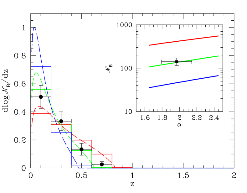
The redshift distribution of the Fermi BL Lac sample (i.e., the First LAT Catalog, 1LAC; Abdo et al., 2010c) is peaked at and falls rapidly thereafter. Inasmuch as the Fermi HSP and ISP counts directly probes the low- , it may appear that they are inconsistent with the rapidly evolving described in the previous section. Indeed, an analysis of the first three months of Fermi observations, suggested that the BL Lac population does not grow substantially with redshift (Abdo et al., 2009). However, as seen in Figure 6, this is not necessarily the case.
Assuming, as we have, that the number of TeV blazars is equal to the the number of hard Fermi gamma-ray blazars, corresponding to ISPs with (comprising roughly half of that class) and HSPs, the expected number observed inside of a given redshift is:
| (31) |
where and are the proper and angular diameter distances, respectively, is the intrinsic upper-cutoff of the TeV blazar isotropic-equivalent luminosity function, and
| (32) | ||||
is lower-limit set by the Fermi flux limit (see Figure 23 of Abdo et al., 2010c, and surrounding discussion). The factor is a correction relating the – isotropic-equivalent luminosities we employ to define to the – luminosities used by Fermi to define the flux limit. The dependence upon arises from the limited spectral coverage of both definitions, though here we fix for all objects based upon the sources that dominate the TeV flux at Earth. Note that since the from Hopkins et al. (2007) diverges at small , the lower-luminosity cutoff is critical to getting both the total number of TeV blazars and the shape of their redshift distribution correct. The resulting is shown in Figure 6 for three different choices of : , , and , of which is most similar to the 1LAC hard gamma-ray blazars.
Generally, our does an excellent job of reproducing the overall number of 1LAC hard gamma-ray blazars and the dominance of nearby objects in their redshift distribution. This is despite the strong redshift evolution of implied by its relationship with . The reason for this is the flat distribution at low , the steep drop-off at high (a result of which is that the shape is only marginally sensitive to the cutoff at ) and the rapidly growing due to the fixed flux limit.
However, we note that the comparison between and the 1LAC hard gamma-ray blazar statistics assumes that those with measured redshifts, comprising roughly half of the 1LAC hard gamma-ray blazar sample, are representative of the hard gamma-ray blazar population as a whole. This appears not to be the case; as we discuss in detail in Appendix C, it is clear that the 1LAC HSPs with and without measured redshifts are not drawn from the same underlying -distribution. Based upon a similar analysis for 1LAC BL Lacs generally, Abdo et al. (2010c) argued that the objects without redshifts are more consistent with population. However, this conclusion does not extend to HSPs, for which there are only three sources in the clean 1LAC HSP sample with . Rather, in Appendix C, we show that the 1LAC HSPs without redshifts are distributed both in spectral index and flux much more similarly with nearby HSPs () than more distant HSPs (). If this is because these sources are intrinsically under-luminous, nearby objects, it could marginally improve the already remarkable comparison between the number of objects implied by our and those observed. However, because the number of predicted 1LAC hard gamma-ray blazars is strongly dependent upon the flux limit, even a marginal increase in either at low luminosities or the effective flux limit results in a that is more strongly weighted at low , potentially allowing even more dramatically evolving luminosity functions. For this reason we conclude that our is broadly consistent with the 1LAC hard gamma-ray blazar distribution, and that Fermi does not, at present, exclude a rapidly evolving in the recent past.
5.3 The TeV Blazar Contribution to the Fermi EGRB
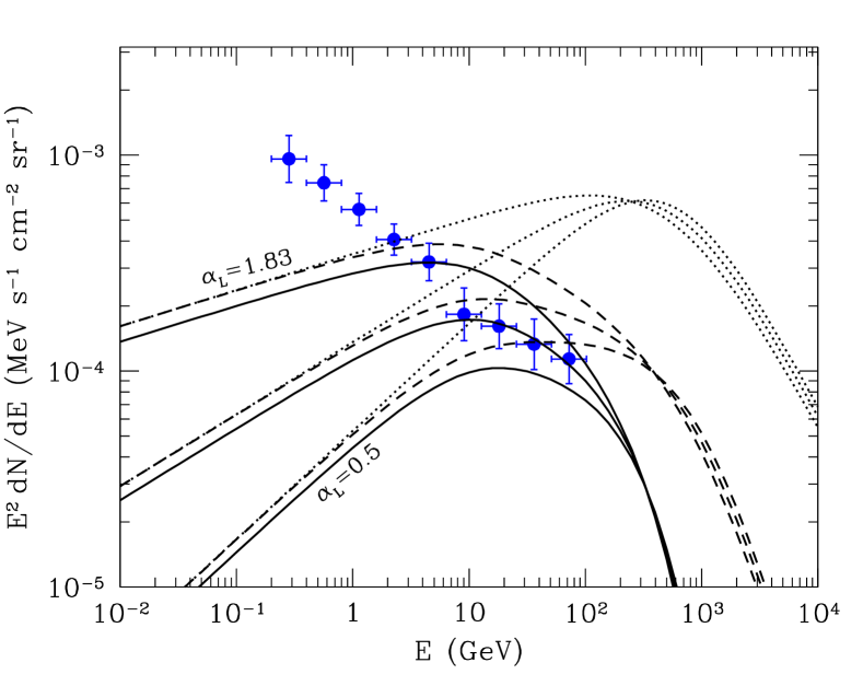
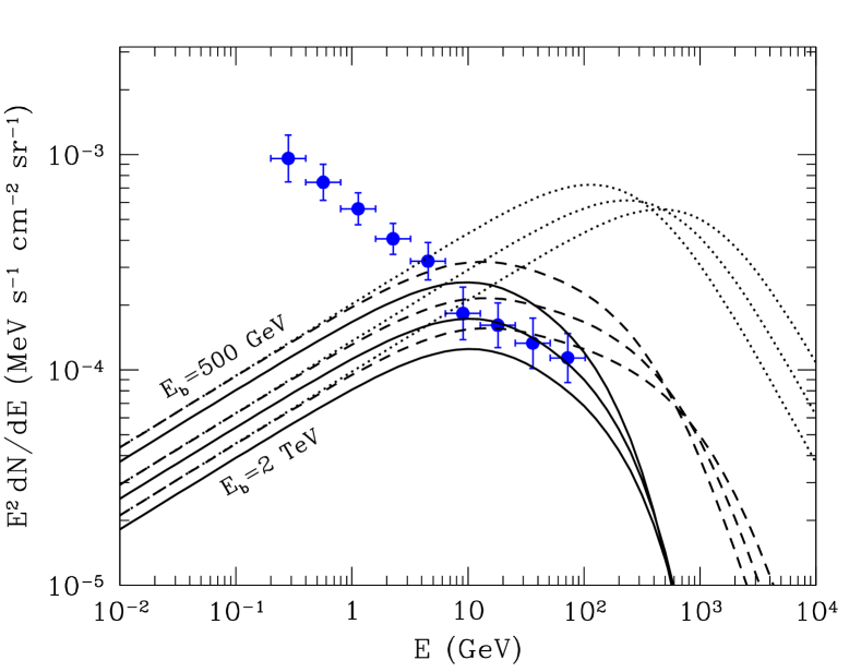
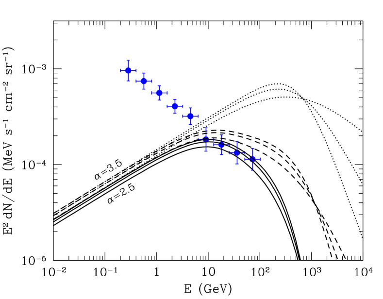
While the statistics of the 1LAC hard gamma-ray blazar sample probes the evolution of at , the Fermi EGRB is sensitive to TeV Blazars at high . The contribution to the EGRB from TeV blazars given our is shown in Figure 7. Because ICCs are suppressed, computing the EGRB flux requires only summing the individual intrinsic spectra of the TeV blazars. For simplicity, to estimate the TeV blazar contribution to the EGRB we assume all TeV blazars have identical intrinsic spectra, given by a broken power law,
| (33) |
where the normalization is set such that the (i.e., , corresponding to the luminosity used to define , and thus determine ), is the energy of the spectral break, and are the low and high-energy spectral indexes, respectively.191919Note that was determined assuming an unbroken spectrum, and thus in this case would over estimate the total flux from the TeV blazars. Nevertheless, here this is not accounted for, i.e., we renormalize the broken power-law spectrum to our previous power-law estimate of the TeV blazar luminosity density. As a consequence, our estimates of the EGRB are also over estimates. With this, after performing the integral over , the EGRB flux is then
| (34) | ||||
where , and is the physical quasar luminosity density. We choose fiducial values for the spectral parameters of , , and , typical of the TeV blazars (see Table 1 and Ghisellini, 2011). Finally, since Fermi resolves individual gamma-ray blazars with isotropic-equivalent luminosities , roughly the location of the peak in , for , we construct the EGRB from sources at larger redshift.
If is sufficiently high () the EGRB is remarkably insensitive to the particular values of and (see the bottom two panels of Figure 7). This is a direct result of the annihilation of the VHEGRs upon the EBL, effectively removing the relevant portion of the blazar SED from the EGRB. More important is the low-energy spectral index. However, for values of that are consistent with the Comptonization models for the VHEGR emission, the anticipated EGRB is consistent with the Fermi result. Thus, we find that despite our dramatically evolving , we are are able to satisfy the limits imposed by the Fermi EGRB. Moreover, for reasonable spectral-parameter values it is possible to accurately reproduce both the magnitude and shape of the high-energy EGRB (i.e., at energies ).202020Note that since we are only presenting the EGRB from the TeV blazars, we necessarily neglect the contributions from the FSRQs and LBLs which dominate the EGRB at low energies. At first this may appear in conflict with other studies that have performed more sophisticated analyses of the gamma-ray emission from blazars (e.g., Narumoto & Totani, 2006; Kneiske & Mannheim, 2008; Inoue & Totani, 2009; Venters, 2010) that have typically found that such a strongly evolving over-produces the Fermi EGRB. However, this is not the case for three reasons.
First, the AGN populations typically considered in computations of the EGRB include the FSRQs and LBLs, which dominate at low energies. The TeV blazars of interest here are only the high-energy tail of the blazar distribution, and it is these alone that we fix to the quasar luminosity function (indeed, it is for only these objects that the arguments surrounding Figure 5 have been made). Moreover, the TeV blazars themselves are generally dimmer, both bolometrically and within the Fermi LAT energy band (–), than the LBLs and FSRQs, which have typical isotropic-equivalent luminosities of (Narumoto & Totani, 2006).
Second, and perhaps most importantly, the suppression of the ICCs means that the VHEGR emission is lost to heat in the IGM, not reprocessed to below . Since the TeV blazar flux is presumed to be dominated by emission above , the non-radiative dissipation of this emission substantially reduces the impact of the TeV blazars upon the EGRB. For all of the spectral parameters we considered the un-absorbed fluxes exceed the EGRB by a significant margin, implying that the suppression of the ICCs is crucial to bringing the TeV blazar contributions in line with the Fermi EGRB. Thus, the lack of the ICCs generally appears necessary to reconcile the blazar and quasar luminosity functions.
Third, the VHEGR spectra from the most luminous TeV blazars necessarily peaks near or above TeV energies. For a number of the sources in Table 1, the intrinsic VHEGR spectrum (adjusted for annihilation on the EBL) is inverted, indicating that this break is above a TeV. The brightest TeV blazar in Table 1, Mkn 421, has an inverted spectrum below (Abdo et al., 2010c), implying . The second brightest, 1ES 1959+650, is consistent with being flat below , and appears to peak near when in the high-state (Daniel et al., 2005). Similarly, 1ES 2344+514 peaks near (Albert et al., 2007c) and Mkn 501 is inverted below , implying a peak above that value (Abdo et al., 2010c). Thus the sources likely to dominate the VHEGR background, and by extension the EGRB, all turn over near –. This is expected if the the VHEGR emission arises from inverse-Compton scattering the synchrotron bump (see, e.g., Ghisellini, 2011, and references therein). The consequence of the spectral break is the suppression of the contribution from the TeV blazars to the EGRB below . Were the TeV blazar contribution to the EGRB dominated by sources with it would exceed the Fermi EGRB at .
A more complete analysis of the EGRB should include a variety of spectra, including a distribution of break energies, smoothly connecting the HBL, IBL and LBL populations. However, this is beyond the scope of this paper, which is primarily concerned with the fate of the VHEGR emission, absent in the LBLs and FSRQs. Nevertheless a recent comprehensive model, which includes the contributions of the FSRQs and BL Lacs observed by Fermi, as well as starburst galaxies, has had considerable success fitting the Fermi EGRB with an even more extremely evolving ; fixing it to the luminosity function of radio galaxies (Cavadini et al., 2011; Stecker & Venters, 2011). Of particular relevance here is that Cavadini et al. (2011) and Stecker & Venters (2011) explicitly ignored the potential contributions of ICCs. Unlike their analysis, however, we find that the TeV blazars are capable of reaching the highest Fermi bands despite the annihilation upon the EBL.
6 Conclusions
The cold, highly anisotropic beams of ultra-relativistic pairs produced by the annihilation of VHEGRs upon the EBL are unstable to plasma beam instabilities. More importantly, for a wide range of parameters relevant for the observed TeV blazars these instabilities may be capable of isotropizing, and potentially extracting the kinetic energy of, the pairs at a rate orders of magnitude faster than inverse-Compton scattering.
This has far reaching consequences for efforts to constrain the IGMF using empirical limits upon the GeV emission from known TeV sources. Typically, after the onset of TeV emission the pair beam density has grown sufficiently for plasma beam instabilities to dominate its evolution, randomize the beam, and potentially suppress the inverse-Compton signal upon which the IGMF limits are based. Note that due to the beam disruption by the instabilities, this occurs even if the plasma instabilities do not ultimately cool the pairs. As a consequence, the present constraints upon the IGMF, obtained by the non-observation of an inverse-Compton GeV bump in the spectra of bright TeV blazars are inherently unreliable. Nevertheless, the sudden appearance of a TeV-bright blazar or intrinsically transient sources (e.g., GRBs) provide a means to temporarily avoid the consequences of plasma beam instabilities during the growth of the pair beam. Alternatively, observing particularly dim sources, , limits the beam density directly, again avoiding the complications imposed by plasma processes. Finally, the presence of these plasma instabilities in the pair beams of TeV blazars, which manifest themselves through their impact on the IGM (see Paper II, Paper III, and Puchwein et al. (2011)), implies the most stringent upper limit to date on the IGMF: .
If the plasma instabilities can efficiently convert the pair beam kinetic energy into heat in the IGM, as we anticipate based upon existing numerical simulations and the arguments in Section 3.5, they would necessarily suppress the development of ICCs, and thus prevent the reprocessing of the VHEGR emission from bright sources to GeV energies. The lack of ICCs, independent of the mechanism that facilitates the local dissipation of the pair kinetic energy, would greatly weaken the constraints upon the evolution of the blazar population derived from the unresolved EGRB measured by Fermi. By introducing a spectral break near and eliminating the reprocessed VHEGR emission, we find that the Fermi EGRB is consistent with a TeV blazar (and therefore presumably hard gamma-ray blazar) luminosity function fixed to that of quasars, normalized by comparing objects in the local Universe (), and motivated by the remarkable similarity between them in the local Universe. This conclusion is relatively insensitive to the particular parameters governing the VHEGR spectra of the TeV blazars, requiring only that the VHEGR emission is produced via inverse-Compton scattering. For a wide range of spectral parameters, we are able to match the magnitude and shape of the Fermi EGRB at high energies, with the low-energy component presumably arising from the FSRQs and LBLs. This , and perhaps an even more rapidly evolving luminosity function, is also consistent with the observed redshift distribution of the 1LAC HSP and hard-ISP sample.
Matching the high-energy EGRB (above ) requires more TeV blazars than are currently observed, though a comparable number to those inferred once the sky-coverage and GeV duty-cycle completeness corrections are included. Based upon these factors, and our rough estimate of the EGRB, we predict that upcoming surveys performed with next-generation Cerenkov telescope arrays (see, e.g., CTA Consortium, 2010) should find roughly sources above (our estimate of the effective flux limit of current imaging Cerenkov telescopes), and a handful of additional sources comparable to the brightest TeV blazars observed. In addition, based upon the current number of known TeV blazars and our estimate of , the improved anticipated sensitivities of these instruments, – time larger than current arrays, should result in the detection of – additional TeV blazars, with median luminosities . These should allow more precise estimates for their gamma-ray SEDs and a better characterization of , especially for low-luminosity objects.
Unlike inverse-Compton cooling, the plasma beam instabilities deposit the energy locally, heating the IGM. Moreover, the homogeneity of the EBL, and the weak dependence of the plasma cooling rates upon the IGM density, result in a uniform volumetric heating, in clear contrast to either photoionization heating or mechanical feedback from AGN. While we shall defer a detailed discussion of the consequences of this heating to Papers II, III, and Puchwein et al. (2011) here we note that this unusual heating prescription naturally explains a number of heretofore outstanding questions, including the inverted equation-of-state (temperature-density relation) for low density regions in the IGM (Paper II), the suppression of dwarf galaxies and their histories, the segregation of galaxy clusters and groups into cool core and non-cool core populations (Paper III), and the quantitative properties of the high-redshift Ly forest (Puchwein et al., 2011). As a consequence, despite the fact that our estimates of the plasma cooling rates are limited to the linear regime (though with some numerical support), there are a variety of observational reasons to believe that plasma cooling, or an analogous mechanism, does in fact dominate the evolution of the ultra-relativistic pair beams.
Acknowledgements.
We thank Tom Abel, Marco Ajello, Marcelo Alvarez, Arif Babul, Roger Blandford, James Bolton, Mike Boylan-Kolchin, Luigi Costamante, Andrei Gruzinov, Peter Goldreich, Martin Haehnelt, Andrey Kravtsov, Ue-li Pen, Ewald Puchwein, Volker Springel, Chris Thompson, Matteo Viel, Marc Voit, and Risa Wechsler for useful discussions. We are indebted to Peng Oh for his encouragement and useful suggestions. We thank Steve Furlanetto for kindly providing technical expertise. These computations were performed on the Sunnyvale cluster at CITA. A.E.B. and P.C. are supported by CITA. A.E.B. gratefully acknowledges the support of the Beatrice D. Tremaine Fellowship. C.P. gratefully acknowledges financial support of the Klaus Tschira Foundation and would furthermore like to thank KITP for their hospitality during the galaxy cluster workshop. This research was supported in part by the National Science Foundation under Grant No. NSF PHY05-51164.Appendix A Instability Growth Rates
Here we compute the growth rates for the various plasma instabilities discussed in the text within the context of relativistically moving pair plasmas. In all cases we make use of the kinetic theory description of the underlying plasmas. This necessarily assumes that the plasma, and in particular the beam plasma, is sufficiently dense that it is well described by a distribution function on the relevant scales. This is equivalent to requiring that many particles within a characteristic energy range be present on the plasma scale of the IGM, i.e., the conditions laid out in Section 3.1. In our analysis the Vlasov equation will play a central role, which owing to the relativistic nature of the calculation, we express in terms of the canonical pair, and , making use of the Lorentz invariance of the electron/positron distribution functions and the phase-space volume element . In what follows we set unless otherwise specified.
A.1 Relativistic Pair Two-Stream Instability
The two-stream instability arises due to the excitation of negative-energy electrostatic waves in the beam and target plasmas. These waves carry away both the energy and momentum of the beam. Specifically, we compute the growth rate of the electrostatic wave moving in the direction of the beam in the absence of a background magnetic field212121Where the beam energy density is large in comparison to that associated with the background magnetic field this is well justified.. In this case, the Vlasov equations for the electrons and positrons are:
| (35) | ||||
where is the Stokes derivative and is the net electric field. Linearizing these and Fourier transforming in and gives
| (36) | ||||
where are the perturbations to the electron and positron distribution functions, is the electrostatic wave field and we have assumed that the background distributions, , are isotropic. As a result we have
| (37) |
At this point we may compute the dielectric tensor associated with the plasma response, however it will suffice to consider Gauss’s law. Thus we now compute the perturbed charge density:
| (38) | ||||
It is now necessary to specify the . We idealize the target ionic plasma as cold and the pair beam plasma as mono-energetic, yielding
| (39) |
where and are the lepton number densities in the target and beam, respectively. After performing the trivial integrals we then obtain
| (40) | ||||
were in the final equality we used the fact that . From Gauss’s law we have , and therefore
| (41) |
where and are the plasma frequencies associated with the target and beam plasmas.
This explicitly provides the dispersion relation, quadratic in (one electrostatic wave traveling in each direction for each plasma). When , . When , as is the case of interest here, we may solve the dispersion relation perturbatively. We do this by setting , with , which gives:
| (42) |
which is no longer independent of . When , is real and thus there is no instability. On the other hand, where , we have
| (43) |
and therefore . This has three solutions:
| (44) |
the first of which is oscillatory, the second is decaying and the third is growing with timescale
| (45) |
This differs from that associated with non-relativistic, ionic beams only by the factor of , arising due to time-dilation within the beam.
Note that since the energy within the electrostatic wave is proportional to , the rate at which energy is removed from the beam is .
A.2 Relativistic Pair Weibel Instability
The relativistic version of the Weibel instability has been discussed in some detail in the literature for the case of anisotropic, though symmetric beams (Weibel, 1959; Fried, 1959; Yoon & Davidson, 1987; Medvedev & Loeb, 1999). Here we consider a the case of a dilute pair beam incident upon a much denser target plasma. This is essentially identical to the two-stream instability discussed previously, though coupling instead to an electromagnetic mode with .
Again we begin with the linearized Vlasov equations for the electrons and positrons:
| (46) | ||||
where we have from Faraday’s law. Fourier transforming in and and solving for gives
| (47) | ||||
The associated perturbation to the current is
| (48) | ||||
in which we’ve defined .
Choosing the given by Equation (39) and assuming we recover the standard two-stream instability. For our purposes here, however, the computations may be substantially simplified by boosting into a frame in which the target plasma is not at rest. In this frame we have given by,
| (49) |
with , where we will take care at the end to properly relate all of these quantities to their target-frame analogs. In particular, we choose this frame such that , where and are the proper densities of the target and beam plasmas, respectively. If is the beam plasma velocity in the target (or lab) frame, this gives
| (50) |
where and is in our case much less than unity. Note that this is only the center of momentum frame if (for which , the case most commonly discussed). If we choose this choice of frame causes the terms linear in in Equation (48) to vanish identically, yielding
| (51) |
Using the inhomogeneous wave equation, obtained from Faraday’s and Ampere’s law,
| (52) |
and choosing produces the dispersion relation
| (53) |
At this point we make use of the fact that in our case , which allows a perturbative solution of Equation (50): and therefore . Furthermore, and for the geometry under consideration. As consequence, and , which implies that
| (54) |
This has a purely imaginary solution:
| (55) |
For this rises linearly with , saturating for , giving the growth rate
| (56) |
Given that for our application , we will drop terms first order in as well. Note that the plasma frequency that enters into the growth rate is that of the beam, which is much lower than that associated with the target plasma. Nevertheless, the scale of the rapidly growing perturbations is limited to that associated with the target plasma, which are general much smaller than that associated with the perturbations in the beam alone. Again, the rate at which energy is sapped from the beam is then .
Appendix B An Explicit Expression for the Quasar Luminosity Function
In the interests of completeness, here we reproduce the from Hopkins et al. (2007), corresponding to the “Full” case in that paper, that we employ. See Hopkins et al. (2007) for how this was obtained, and caveats regarding its application.
cccccccc\tabletypesize
\tablecaptionParameters of the Quasar Luminosity Function from Hopkins et al. (2007)
\tablehead
Normalization
\startdata \tablenotemarka &
\tablenotemarkb
\enddata\tablenotetextaIn units of comoving
\tablenotetextbIn units of
The form of is assumed to be a broken power law:
| (57) |
where the location of the break () and the power laws ( and ) are functions of redshift. These are given by,
| (58) | ||||
where
| (59) |
The values of the relevant parameters are given in Table B, and where any estimate of the uncertainty is made we assume these are independently, normally distributed.
Appendix C Inferring the Redshift Distribution of the Fermi HSPs without Measured Redshifts
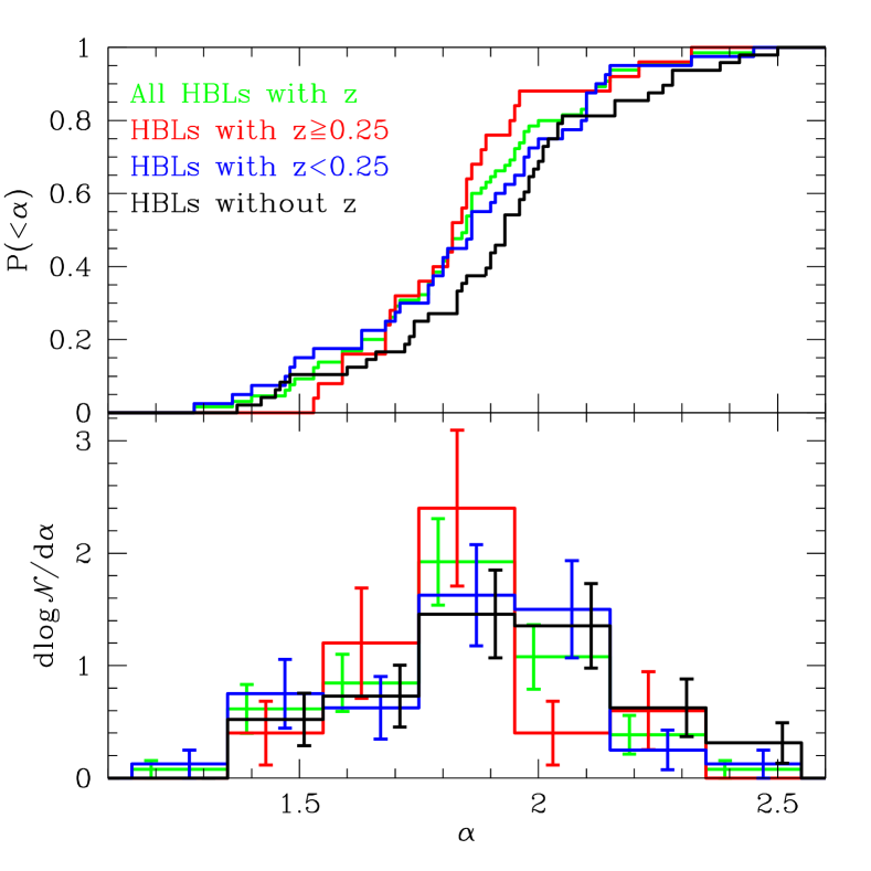
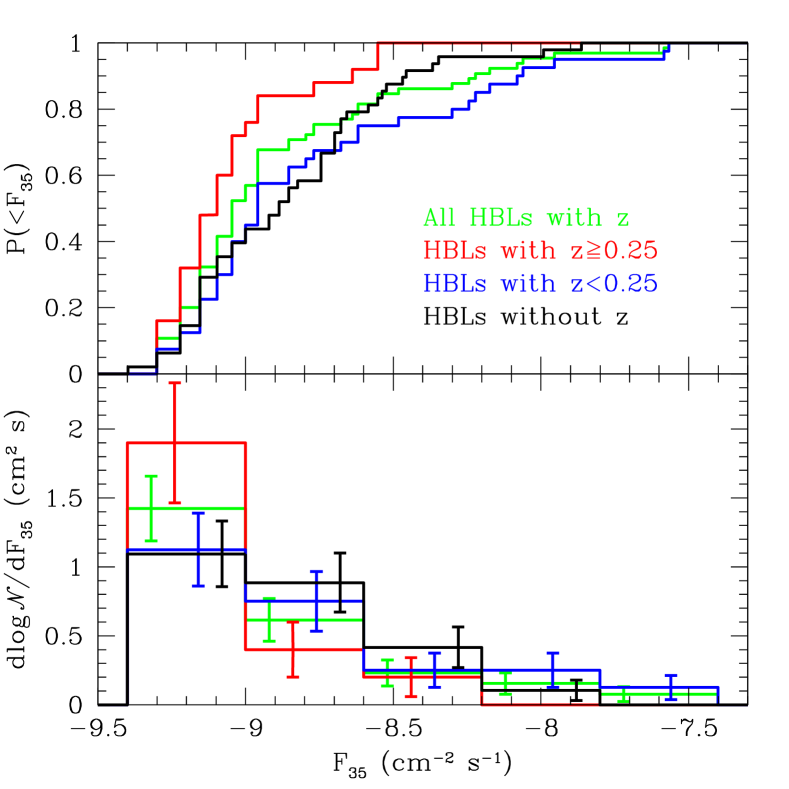
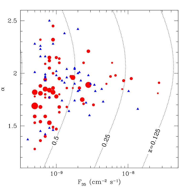
| Redshift | Spectral Index | Flux between – | ||
|---|---|---|---|---|
| Population | ||||
| All HSPs with ’s | ||||
| HSPs with | ||||
| HSPs with | ||||
| HSPs without ’s | — | — | ||
Of the 118 HSPs detected by Fermi and reported in the First LAT AGN Catalog (1LAC, Abdo et al., 2010c, , there called HSPs), 113 are members of the clean sample (meaning that there are no ambiguities surrounding their detection), and of these only 65 have measured redshifts. This is a somewhat larger fraction that for 1LAC BL Lacs generally, though this leaves nearly half of the HSP population with their redshifts undetermined. Based upon comparisons between the spectral index and flux distributions between the HSPs without redshifts and those at various redshift ranges, here we argue that these are likely to be located nearby.
Already, based upon comparisons between the spectral index distributions (SIDs) of the 1LAC BL Lacs at large, it is clear that the objects with and without measured redshifts are not drawn from the same underlying population (Abdo et al., 2010c). Similarities between the SIDs of the unknown- objects and the subset of those with measured redshifts, Abdo et al. (2010c) has suggested that the BL Lacs without redshifts may be biased towards higher redshifts. However, we note that there are only three HSPs with , and thus this conclusion is relevant for ISPs and LSPs only.
The SIDs of the unknown- HSPs is shown in Figure 8, compared with the SIDs of HSPs with redshifts (cf. Figure 22 of Abdo et al., 2010c). The Kolmogorov-Smirnov (KS) probability that these are drawn from the same parent population is , indicating that this is unlikely at the 2- level. In addition, we show the SIDs of HSPs with (blue line) and (red line), with corresponding KS probabilities of and , respectively (these are collected in Table 1). Thus, in contrast to the 1LAC BL Lac sample at large, the HSPs without redshifts appear to have SIDs that are strongly inconsistent with the population observed to have high redshifts, and indistinguishable from those at low redshifts. Nevertheless, the HSPs with unknown-s still tend to be softer than those with measured redshifts in either range.
A similar analysis may be performed upon the reported flux measure, , corresponding to the flux between and . Figure 9 shows the flux distributions (FDs) of the unknown-, all measured , , and HSP populations, and is analogous to Figure 8. As before, the HSPs without redshifts have FDs that are marginally inconsistent with being drawn from the same parent population as the complete set of HSPs with measured redshifts, having a KS probability of . The inconsistency with the high- HSP FD is even more striking than for the SIDs, with a KS probability less than , i.e., that the high- FD of the unknown- and HSPs are from the same distribution is excluded. However, again, we find that the FDs of the low- and unknown- populations are indistinguishable, having a KS probability of .
That the SIDs and FDs both favor a relationship between the unknown- and low- HSP populations provides some confidence that this may, in fact, be the case. This is supported by the redshift distribution in the - plane, depicted in Figure 10. HSPs with high redshifts are clustered at low fluxes and hard . This is not unexpected given an upper limit upon the luminosity of HSPs. The dotted lines in Figure 10 show constant redshift curves in the – plane for a – luminosity of (the definition of in Abdo et al., 2010c, note the distinction with the definition of ). If all HSPs have intrinsic luminosities less than , no sources at a given should be found to the right of the associated line. Since the volume of the visible Universe is dominated by , the majority of high- objects should then be found up against the instrumental flux limit, i.e., at low fluxes and nearly flat spectra. Sources with harder spectra are likely to have higher bolometric gamma-ray luminosities since they are likely to be more below the inverse-Compton peak, biasing high- sources towards harder spectra.
However, the HSPs without redshifts are noticeably absent within this high- dominated region. This is responsible for the fact that they more closely share their SID and FD with the low- HSPs. The presence of HSPs without redshifts at a variety of s and s suggests that this is not a result of a selection effect upon either. It is nonetheless possible that there is some instrumental effect which prevents the measurement of high redshifts in intrinsically bright, soft objects, in which case a population of high-luminosity HSPs with high (and therefore unmeasured) s would necessarily be located in regions with predominantly low measured s. However, this is belied by the broad distribution of luminosities and spectral indexes among the HSPs with measured redshifts. Thus, we adopt the simpler explanation: the HSPs with unknown redshifts have and SID and FD similar to low- objects because they are intrinsically dim, nearby objects.
References
- Abdo et al. (2009) Abdo, A. A., et al. 2009, ApJ, 700, 597
- Abdo et al. (2010a) —. 2010a, Phys. Rev. Lett., 104, 101101
- Abdo et al. (2010b) —. 2010b, ApJ, 720, 435
- Abdo et al. (2010c) —. 2010c, ApJ, 715, 429
- Abdo et al. (2010d) —. 2010d, ApJ, 716, 30
- Acciari et al. (2009a) Acciari, V., et al. 2009a, ApJ, 690, L126
- Acciari et al. (2008) Acciari, V. A., et al. 2008, ApJ, 679, 397
- Acciari et al. (2009b) —. 2009b, ApJ, 707, 612
- Acciari et al. (2009c) —. 2009c, ApJ, 693, L104
- Acciari et al. (2010a) —. 2010a, ApJ, 709, L163
- Acciari et al. (2010b) —. 2010b, ApJ, 708, L100
- Acciari et al. (2010c) —. 2010c, ApJ, 715, L49
- Aharonian et al. (2002) Aharonian, F., et al. 2002, A&A, 384, L23
- Aharonian et al. (2003) —. 2003, A&A, 406, L9
- Aharonian et al. (2005) —. 2005, A&A, 436, L17
- Aharonian et al. (2006) —. 2006, A&A, 455, 461
- Aharonian et al. (2007a) —. 2007a, A&A, 470, 475
- Aharonian et al. (2007b) —. 2007b, A&A, 473, L25
- Aharonian et al. (2007c) —. 2007c, A&A, 475, L9
- Aharonian et al. (2008a) —. 2008a, A&A, 481, L103
- Aharonian et al. (2008b) —. 2008b, A&A, 477, 481
- Aharonian et al. (2010) —. 2010, A&A, 521, 69
- Albert et al. (2006) Albert, J., et al. 2006, ApJ, 648, L105
- Albert et al. (2007a) —. 2007a, ApJ, 666, L17
- Albert et al. (2007b) —. 2007b, ApJ, 667, L21
- Albert et al. (2007c) —. 2007c, ApJ, 662, 892
- Aleksić et al. (2010) Aleksić, J., et al. 2010, ApJ, 723, L207
- Aliu et al. (2009) Aliu, E., et al. 2009, ApJ, 692, L29
- Ando & Kusenko (2010) Ando, S., & Kusenko, A. 2010, ApJ, 722, L39
- Barrow et al. (1997) Barrow, J. D., Ferreira, P. G., & Silk, J. 1997, Physical Review Letters, 78, 3610
- Boyd & Sanderson (2003) Boyd, T. J. M., & Sanderson, J. J. 2003, The Physics of Plasmas (Cambridge: Cambridge University Press)
- Bret (2009) Bret, A. 2009, ApJ, 699, 990
- Bret et al. (2004) Bret, A., Firpo, M., & Deutsch, C. 2004, Phys. Rev. E, 70, 046401
- Bret et al. (2005a) —. 2005a, Physical Review Letters, 94, 115002
- Bret et al. (2005b) —. 2005b, Phys. Rev. E, 72, 016403
- Bret et al. (2010a) Bret, A., Gremillet, L., & Bénisti, D. 2010a, Phys. Rev. E, 81, 036402
- Bret et al. (2010b) Bret, A., Gremillet, L., & Dieckmann, M. E. 2010b, Physics of Plasmas, 17, 120501
- Cavadini et al. (2011) Cavadini, M., Salvaterra, R., & Haardt, F. 2011, arXiv:1105.4613
- Chandra et al. (2010) Chandra, P., et al. 2010, Journal of Physics G Nuclear Physics, 37, 125201
- Chang et al. (2012) Chang, P., Broderick, A. E., & Pfrommer, C. 2012, ApJ in print, arXiv:1106.5504
- Chang et al. (2008) Chang, P., Spitkovsky, A., & Arons, J. 2008, ApJ, 674, 378
- Costamante et al. (2007) Costamante, L., Aharonian, F., & Khangulyan, D. 2007, in American Institute of Physics Conference Series, Vol. 921, The First GLAST Symposium, ed. S. Ritz, P. Michelson, & C. A. Meegan, 157–159
- CTA Consortium (2010) CTA Consortium, T. 2010, arXiv:1008.3703
- Dai & Lu (2002) Dai, Z. G., & Lu, T. 2002, ApJ, 580, 1013
- Daniel et al. (2005) Daniel, M. K., et al. 2005, ApJ, 621, 181
- Davidson et al. (1972) Davidson, R. C., Hammer, D. A., Haber, I., & Wagner, C. E. 1972, Physics of Fluids, 15, 317
- de Angelis et al. (2008) de Angelis, A., Persic, M., & Roncadelli, M. 2008, Modern Physics Letters A, 23, 315
- Dermer et al. (2011) Dermer, C. D., Cavadini, M., Razzaque, S., Finke, J. D., Chiang, J., & Lott, B. 2011, ApJ, 733, L21
- Dolag et al. (2011) Dolag, K., Kachelriess, M., Ostapchenko, S., & Tomàs, R. 2011, ApJ, 727, L4
- Franceschini et al. (2008) Franceschini, A., Rodighiero, G., & Vaccari, M. 2008, A&A, 487, 837
- Frederiksen et al. (2004) Frederiksen, J. T., Hededal, C. B., Haugbølle, T., & Nordlund, Å. 2004, ApJ, 608, L13
- Fried (1959) Fried, B. D. 1959, Physics of Fluids, 2, 337
- Ghisellini (1999) Ghisellini, G. 1999, Astrophysical Letters Communications, 39, 17
- Ghisellini (2011) —. 2011, arXiv: 1104.0006
- Ghisellini et al. (2009) Ghisellini, G., Maraschi, L., & Tavecchio, F. 2009, MNRAS, 396, L105
- Ghisellini & Tavecchio (2008) Ghisellini, G., & Tavecchio, F. 2008, MNRAS, 387, 1669
- Gould & Schréder (1967) Gould, R. J., & Schréder, G. P. 1967, Physical Review, 155, 1408
- Guetta & Granot (2003) Guetta, D., & Granot, J. 2003, ApJ, 585, 885
- HESS Collaboration et al. (2010) HESS Collaboration et al. 2010, A&A, 520, 83
- Hopkins et al. (2007) Hopkins, P. F., Richards, G. T., & Hernquist, L. 2007, ApJ, 654, 731
- Huang et al. (2009) Huang, D., Konopelko, A., & for the VERITAS collaboration. 2009, arXiv: 0912.3772
- Inoue & Totani (2009) Inoue, Y., & Totani, T. 2009, ApJ, 702, 523
- Kandus et al. (2011) Kandus, A., Kunze, K. E., & Tsagas, C. G. 2011, Phys. Rep., 505, 1
- Kneiske et al. (2004) Kneiske, T. M., Bretz, T., Mannheim, K., & Hartmann, D. H. 2004, A&A, 413, 807
- Kneiske & Mannheim (2008) Kneiske, T. M., & Mannheim, K. 2008, A&A, 479, 41
- Komatsu et al. (2011) Komatsu, E., et al. 2011, ApJS, 192, 18
- Kotera & Lemoine (2008) Kotera, K., & Lemoine, M. 2008, Phys. Rev. D, 77, 123003
- Lemoine & Pelletier (2010) Lemoine, M., & Pelletier, G. 2010, MNRAS, 402, 321
- Lesch & Schlickeiser (1987) Lesch, H., & Schlickeiser, R. 1987, A&A, 179, 93
- MAGIC Collaboration et al. (2008a) MAGIC Collaboration et al. 2008a, Science, 320, 1752
- MAGIC Collaboration et al. (2008b) —. 2008b, Science, 320, 1752
- Mariotti & MAGIC Collaboration (2010) Mariotti, M., & MAGIC Collaboration. 2010, The Astronomer’s Telegram, 2916, 1
- Massaro et al. (2009) Massaro, E., Giommi, P., Leto, C., Marchegiani, P., Maselli, A., Perri, M., Piranomonte, S., & Sclavi, S. 2009, A&A, 495, 691
- Medvedev & Loeb (1999) Medvedev, M. V., & Loeb, A. 1999, ApJ, 526, 697
- Melrose (1980) Melrose, D. B. 1980, Plasma astrophysics: Nonthermal processes in diffuse magnetized plasmas. Volume 2 - Astrophysical applications
- Mose Mariotti (2010) Mose Mariotti, M. 2010, The Astronomer’s Telegram, 2684, 1
- Nakar et al. (2011) Nakar, E., Bret, A., & Milosavljevic, M. 2011, ArXiv 1104.5249
- Narumoto & Totani (2006) Narumoto, T., & Totani, T. 2006, ApJ, 643, 81
- Neronov & Semikoz (2009) Neronov, A., & Semikoz, D. V. 2009, Phys. Rev. D, 80, 123012
- Neronov et al. (2011) Neronov, A., Semikoz, D. V., Tinyakov, P. G., & Tkachev, I. I. 2011, A&A, 526, 90
- Neronov & Vovk (2010) Neronov, A., & Vovk, I. 2010, Science, 328, 73
- Oh (2001) Oh, S. P. 2001, ApJ, 553, 25
- Padovani & Giommi (1995) Padovani, P., & Giommi, P. 1995, ApJ, 444, 567
- Pfrommer et al. (2012) Pfrommer, C., Chang, P., & Broderick, A. E. 2012, ApJ in print, arXiv:1106.5505
- Plaga (1995) Plaga, R. 1995, Nature, 374, 430
- Puchwein et al. (2011) Puchwein, E., Pfrommer, C., Springel, V., Broderick, A. E., & Chang, P. 2011, arXiv:1107.3837
- Raue et al. (2010) Raue, M., et al. 2010, in Astronomical Society of the Pacific Conference Series, Vol. 427, Astronomical Society of the Pacific Conference Series, ed. L. Maraschi, G. Ghisellini, R. Della Ceca, & F. Tavecchio, 302
- Salamon & Stecker (1998) Salamon, M. H., & Stecker, F. W. 1998, ApJ, 493, 547
- Silva et al. (2003) Silva, L. O., Fonseca, R. A., Tonge, J. W., Dawson, J. M., Mori, W. B., & Medvedev, M. V. 2003, ApJ, 596, L121
- Spitkovsky (2008) Spitkovsky, A. 2008, ApJ, 682, L5
- Sreekumar et al. (1998) Sreekumar, P., et al. 1998, ApJ, 494, 523
- Stecker & Venters (2011) Stecker, F., & Venters, T. M. 2011, ApJ, 736, 40
- Stecker et al. (1992) Stecker, F. W., de Jager, O. C., & Salamon, M. H. 1992, ApJ, 390, L49
- Strong et al. (2004) Strong, A. W., Moskalenko, I. V., & Reimer, O. 2004, ApJ, 613, 956
- Sturrock (1994) Sturrock, P. A. 1994, Plasma Physics, An Introduction to the Theory of Astrophysical, Geophysical and Laboratory Plasmas (Cambridge: Cambridge University Press)
- Takahashi et al. (2012) Takahashi, K., Mori, M., Ichiki, K., & Inoue, S. 2012, ApJ, 744, L7
- Takahashi et al. (2008) Takahashi, K., Murase, K., Ichiki, K., Inoue, S., & Nagataki, S. 2008, ApJ, 687, L5
- Tavecchio & Ghisellini (2008) Tavecchio, F., & Ghisellini, G. 2008, MNRAS, 386, 945
- Tavecchio et al. (2011) Tavecchio, F., Ghisellini, G., Bonnoli, G., & Foschini, L. 2011, MNRAS, 414, 3566
- Tavecchio et al. (2010) Tavecchio, F., Ghisellini, G., Foschini, L., Bonnoli, G., Ghirlanda, G., & Coppi, P. 2010, MNRAS, 406, L70
- Taylor et al. (2011) Taylor, A. M., Vovk, I., & Neronov, A. 2011, A&A, 529, A144
- Tramacere et al. (2009) Tramacere, A., Giommi, P., Perri, M., Verrecchia, F., & Tosti, G. 2009, A&A, 501, 879
- Urry & Padovani (1995) Urry, C. M., & Padovani, P. 1995, PASP, 107, 803
- Vallée (2011) Vallée, J. P. 2011, New Astron. Rev., 55, 91
- Venters (2010) Venters, T. M. 2010, ApJ, 710, 1530
- Waxman & Miralda-Escude (1996) Waxman, E., & Miralda-Escude, J. 1996, ApJ, 472, L89+
- Weibel (1959) Weibel, E. S. 1959, Physical Review Letters, 2, 83
- Widrow (2002) Widrow, L. M. 2002, Reviews of Modern Physics, 74, 775
- Yoon & Davidson (1987) Yoon, P. H., & Davidson, R. C. 1987, Phys. Rev. A, 35, 2718