Impacts of Collective Neutrino Oscillations on Core-Collapse Supernova Explosions

Abstract

By performing a series of one- and two-dimensional (1-, 2D) hydrodynamic simulations with spectral neutrino transport, we study possible impacts of collective neutrino oscillations on the dynamics of core-collapse supernovae. To model the spectral swapping which is one of the possible outcome of the collective neutrino oscillations, we parametrize the onset time when the spectral swap begins, the radius where the spectral swap occurs, and the threshold energy above which the spectral interchange between heavy-lepton neutrinos and electron/anti-electron neutrinos takes place, respectively. By doing so, we systematically study how the neutrino heating enhanced by the spectral swapping could affect the shock evolution as well as the matter ejection. We also investigate the progenitor dependence using a suite of progenitor models (13, 15, 20, and 25 $M_{\odot}$). We find that there is a critical heating rate induced by the spectral swapping to trigger explosions, which significantly differs between the progenitors. The critical heating rate is generally smaller for 2D than 1D due to the multidimensionality that enhances the neutrino heating efficiency. For the progenitors employed in this paper, the final remnant masses are estimated to range in 1.1-1.5$M_{\odot}$. For our 2D model of the $15M_{\odot}$ progenitor, we find a set of the oscillation parameters that could account for strong supernova explosions ($\sim 10^{51}$ erg), simultaneously leaving behind the remnant mass close to $\sim 1.4M_{\odot}$.

1. Introduction

Although the explosion mechanism of core-collapse supernovae is not completely understood yet, current multi-dimensional (multi-D) simulations based on refined numerical models show several promising scenarios. Among the candidates are the neutrino heating mechanism aided by convection and standing accretion shock instability (SASI) (e.g., Marek & Janka, 2009; Bruenn et al., 2009; Suwa et al., 2010), the acoustic mechanism (Burrows et al., 2007b), or the magnetohydrodynamic (MHD) mechanism (e.g., Kotake et al., 2004, 2006; Obergaulinger et al., 2006; Burrows et al., 2007a; Takiwaki et al., 2009). Probably the best-studied one is the neutrino heating mechanism, whose basic concept was first proposed by Colgate & White (1966), and later reinforced by Bethe & Wilson (1985) to take a currently prevailing delayed form.

An important lesson from the multi-D simulations mentioned above is that hydrodynamic motions associated with convective overturn (Herant et al., 1994; Burrows et al., 1995; Janka & Mueller, 1996; Fryer & Warren, 2002, 2004) as well as the SASI (e.g., Blondin et al., 2003; Scheck et al., 2006; Ohnishi et al., 2006; Foglizzo et al., 2007; Murphy & Burrows, 2008; Iwakami et al., 2008; Guilet et al., 2010; Fernández, 2010) can help the onset of the neutrino-driven explosion, which otherwise fails generally in spherically symmetric (1D) simulations (Liebendörfer et al., 2001; Rampp & Janka, 2002; Thompson et al., 2003; Sumiyoshi et al., 2005). This is mainly because the accretion timescale of matter in the gain region can be longer than in the 1D case, which enhances the strength of neutrino-matter coupling there.

In fact, the neutrino-driven explosions have been obtained in the following state-of-the-art two-dimensional (2D) simulations. Using the MuDBaTH code which includes one of the best available neutrino transfer approximations, Buras et al. (2006) firstly reported explosions for a non-rotating low-mass ($11.2M_{\odot}$) progenitor of Woosley et al. (2002), and then for a $15M_{\odot}$ progenitor of Woosley & Weaver (1995) with a moderately rapid rotation imposed (Marek & Janka, 2009). By implementing a multi-group flux-limited diffusion algorithm to the CHIMERA code (e.g., Bruenn et al., 2009), Yakunin et al. (2010) obtained explosions for a non-rotating $12M_{\odot}$ and 25$M_{\odot}$ progenitor of Woosley et al. (2002). More recently, Suwa et al. (2010) pointed out that a stronger explosion is obtained for a rapidly rotating $13M_{\odot}$ progenitor of Nomoto & Hashimoto (1988) compared to the corresponding non-rotating model, in which the isotropic diffusion source approximation (IDSA) for the spectral neutrino transport (Liebendörfer et al., 2009) is implemented in the ZEUS code.

However, this success opens further new questions. First of all, the explosion energies obtained in these simulations are typically underpowered by one or two orders of magnitudes to explain the canonical supernova kinetic energy ($\sim 10^{51}$ erg). Moreover, the softer nuclear equation of state (EOS), such as of the Lattimer & Swesty (1991) (LS) EOS with an incompressibility $K=180$ MeV at nuclear densities is employed in those simulations. On top of evidence that favors a stiffer EOS based on nuclear experimental data (Shlomo et al., 2006), the soft EOS may not account for the recently observed massive neutron star of $\sim 2M_{\odot}$ (Demorest et al., 2010) (see the maximum mass for the LS180 EOS in O’Connor & Ott, 2011). With a stiffer EOS, the explosion energy may be even lower as inferred from Marek & Janka (2009) who did not obtain the neutrino-driven explosion for their model with $K=263$ MeV. What is then missing furthermore? We may get the answer by going to 3D simulations (Nordhaus et al., 2010) or by taking into account new ingredients, such as exotic physics in the core of the protoneutron star (Sagert et al., 2009), viscous heating by the magnetorotational instability (Thompson et al., 2005; Masada et al., 2011), or energy dissipation via Alfvén waves (Suzuki et al., 2008).

Joining in these efforts, we explore in this study the possible impacts of collective neutrino oscillations on energizing the neutrino-driven explosions. The collective neutrino oscillations, i.e. neutrinos of all energies that oscillate almost in phase, are attracting great attention, because they can induce dramatic observable effects such as a spectral split or swap (e.g., Raffelt & Smirnov, 2007; Duan et al., 2008; Dasgupta et al., 2008, and see references therein). They are predicted to emerge as a distinct feature in their energy spectra (see Duan et al., 2010; Dasgupta, 2010, for reviews of the rapidly growing research field and collective references therein). Among a number of important effects possibly created by the self-interaction, we choose to consider the effect of spectral splits between electron- ($\nu_{e}$), anti-electron neutrinos ($\bar{\nu}_{e}$), and heavy lepton neutrinos ($\nu_{x}$, i.e., $\nu_{\mu}$, $\nu_{\tau}$ and their anti-particles) above a threshold energy (e.g., Fogli et al. (2007)). Since $\nu_{x}$’s have higher average energies than the other species in the postbounce phase, the neutrino flavor mixing would increase the effective energies of $\nu_{e}$ and $\bar{\nu}_{e}$, and hence increase the neutrino heating rates in the gain region. A formalism to treat the neutrino oscillation in the Boltzmann neutrino transport is given in Yamada (2000); Strack & Burrows (2005), but difficult to implement. To just mimic the effects in this study, we perform the spectral swap by hand as a first step. By changing the average neutrino energy, $\left<\epsilon_{\nu_{x}}\right>$, as well as the position of the neutrino spheres ($R_{\nu_{x}}$) in a parametric manner, we hope to constrain the parameter regions spanned by $\left<\epsilon_{\nu_{x}}\right>$ and $R_{\nu_{x}}$ in which the additional heating given by the collective neutrino oscillations could have impacts on the explosion dynamics. Our strategy is as follows. By performing a number of 1D simulations, we will firstly constrain the parameter regions to some extent. Here we also investigate the progenitor dependence using a suite of progenitor models (13, 15, 20, and 25 $M_{\odot}$). After squeezing the condition in the 1D computations, we include the flavor conversions in 2D simulations to see their impacts on the dynamics, and we also discuss how the critical condition for the collective effects in 1D can be subject to change in 2D.

The paper opens with descriptions of the initial models and the numerical methods focusing how to model the collective neutrino oscillations (Section 2). The main results are shown in Section 3. We summarize our results and discuss their implications in Section 4.

2. Numerical Methods

2.1. Hydrodynamics

The employed numerical methods are essentially the same as those in our previous paper (Suwa et al., 2010). For later convenience, we briefly summarize them in the following. The basic evolution equations are written as,

$$\frac{\mathrm{d}\rho}{\mathrm{d}t}+\rho\nabla\cdot\mathbf{v}=0,$$ (1)

$$\rho\frac{\mathrm{d}\mathbf{v}}{\mathrm{d}t}=-\nabla P-\rho\nabla\Phi,$$ (2)

$$\frac{\mathrm{d}e^{*}}{\mathrm{d}t}+\nabla\cdot\left[\left(e^{*}+P\right)\mathbf{v}\right]=-\rho\mathbf{v}\cdot\nabla\Phi+Q_{E},$$ (3)

$$\frac{{\mathrm{d}Y_{e}}}{\mathrm{d}t}=Q_{N},$$ (4)

$$\bigtriangleup{\Phi}=4\pi G\rho,$$ (5)

where $\rho,\mathbf{v},P,\mathbf{v},e^{*},\Phi$, are density, fluid velocity, gas pressure including the radiation pressure of neutrinos, total energy density, gravitational potential, respectively. The time derivatives are Lagrangian. As for the hydro solver, we employ the ZEUS-2D code (Stone & Norman, 1992) which has been modified for core-collapse simulations (e.g., Suwa et al., 2007b, a, 2009; Takiwaki et al., 2009). $Q_{E}$ and $Q_{N}$ (in Equations (3) and (4)) represent the change of energy and electron fraction ($Y_{e}$) due to the interactions with neutrinos. To estimate these quantities, we implement spectral neutrino transport using the isotropic diffusion source approximation (IDSA) scheme (Liebendörfer et al., 2009). The IDSA scheme splits the neutrino distribution into two components, both of which are solved using separate numerical techniques. We apply the so-called ray-by-ray approach in which the neutrino transport is solved along a given radial direction assuming that the hydrodynamic medium for the direction is spherically symmetric. Although the current IDSA scheme does not yet include $\nu_{x}$ and the inelastic neutrino scattering with electrons, these simplifications save a significant amount of computational time compared to the canonical Boltzmann solvers (see Liebendörfer et al. (2009) for more details). Following the prescription in Müller et al. (2010), we improve the accuracy of the total energy conservation by using a conservation form in equation (3), instead of solving the evolution of internal energy as originally designed in the ZEUS code. Numerical tests are presented in Appendix A.

The simulations are performed on a grid of 300 logarithmically spaced radial zones from the center up to 5000 km and 128 equidistant angular zones covering $0\leq\theta\leq\pi$ for two-dimensional simulations. For the spectral transport, we use 20 logarithmically spaced energy bins reaching from 3 to 300 MeV.

2.2. Spectral swapping

As mentioned in §1, we introduce a spectral interchange from heavy-lepton neutrinos ($\nu_{\mu}$, $\nu_{\tau}$ and their antineutrinos, collectively referred as $\nu_{x}$ hereafter) to electron-type neutrinos and antineutrinos, namely $\nu_{x}\rightarrow\nu_{e}$ and $\bar{\nu}_{x}\rightarrow\bar{\nu}_{e}$. Instead of solving the transport equations for $\nu_{x}$, we employ the so-called light-bulb approximation and focus on the optically thin region outside the neutrinosophere (e.g., Janka & Mueller, 1996; Ohnishi et al., 2006).

According to Duan et al. (2010), we set the threshold energy, $\epsilon_{th}$, to be 9 MeV, above which the spectral swap takes place. Below the threshold, the neutrino heating is estimated by the spectral transport via the IDSA scheme. Above the threshold, the heating rate is replaced by

$$Q_{E}\propto\int^{\infty}_{\epsilon_{th}}d\epsilon_{\nu}~{}\epsilon^{3}\left[j(\epsilon_{\nu})+\chi(\epsilon_{\nu})\right]f_{\nu}(r,\epsilon_{\nu}),$$ (6)

where $j$ and $\chi$ are the neutrino emissivity and absorptivity, respectively, and $f_{\nu}(r,\epsilon_{\nu})$ corresponds to the neutrino distribution function for $\nu_{x}$ with $\epsilon_{\nu}$ being energies of electron neutrinos and antineutrinos. In the light-bulb approach, it is often approximated by the Fermi-Dirac distribution with a vanishing chemical potential (e.g., Ohnishi et al., 2006) as,

$$f_{\nu}(r,\epsilon_{\nu})=\frac{1}{e^{\epsilon_{\nu}/kT_{\nu_{x}}}+1}g(r),$$ (7)

where $k$, $T_{\nu_{x}}$ are the Boltzmann constatn and the neutrino temperature, respectively. $g(r)$ is the geometric factor, $g(r)=1-\left[1-(R_{\nu_{x}}/r)^{2}\right]^{1/2}$ which is taken into account for the normalization, with $R_{\nu_{x}}$ being the radius of the neutrinosphere. The neutrino luminosity of $\nu_{x}$ at the infinity is the given as

$$L_{\nu_{x}}=2.62\times 10^{52}\left(\frac{\left<\epsilon_{\nu_{x}}\right>}{15~{}\mathrm{MeV}}\right)^{4}\left(\frac{R_{\nu_{x}}}{30~{}\mathrm{km}}\right)^{2}~{}\mathrm{erg~{}s^{-1}},$$ (8)

where $\left<\epsilon_{\nu_{x}}\right>=\int^{\infty}_{0}d\epsilon_{\nu_{x}}\epsilon_{\nu_{x}}^{3}f_{\nu}(\epsilon_{\nu_{x}})/\int^{\infty}_{0}d\epsilon_{\nu_{x}}\epsilon_{\nu_{x}}^{2}f_{\nu}(\epsilon_{\nu_{x}})$ is the average energy of emitted neutrinos. The position where the spectral swapping sets in is fixed at 100 km (around the gain radius) and the onset time is varied as a parameter, $t_{s}=$100, 200, and 300 ms after bounce.

In fact, the threshold energy depends on the neutrino luminosities, spectra and oscillation parameters (see, e.g., Duan et al., 2010, and references therein) with conserved net $\nu_{e}$ flux (i.e., the lepton number conservation). However, the conservation of lepton number is too complicated to satisfy in the dynamical simulation because the neutrino spectrum and the luminosity evolve with time. In order to focus on the hydrodynamic features affected by the spectral modulation induced by the swapping, we simplify just a single threshold energy in this work.

To summarize, the parameters that we use to mimic the spectral swapping are the following three items, (i) $R_{\nu_{x}}$ which is the radius of the neutrinosphere of $\nu_{x}$, (ii) $\left<\epsilon_{\nu_{x}}\right>$ which is the average energy of $\nu_{x}$, and (iii) $t_{s}$ which is the time when the spectral swapping sets in.

3. Result

3.1. One-dimensional models

3.1.1 1D without spectral swapping

In this subsection, we first outline the 1D collapse dynamics without spectral swapping. We take a 13 $M_{\odot}$ progenitor (Nomoto & Hashimoto, 1988) as a reference.

At around 112 ms after the onset of gravitational collapse, the bounce shock forms at a radius of $\sim$ 10 km with an enclosed mass of $\sim 0.7M_{\odot}$. The central density at this time is $\rho_{c}=3.6\times 10^{14}$ g cm^-3. The shock propagates outwards but finally stalls at a radius of $\sim$ 100 km. Due to the decreasing accretion rate through the stalled shock, the shock can be still pushed outward. However, after some time, the shock radius begins to shrink. The ratio of the advection timescale, $\tau_{\mathrm{adv}}$, and the heating timescale, $\tau_{\mathrm{heat}}$, is an important indicator for the criteria of neutrino driven explosion (Buras et al., 2006; Marek & Janka, 2009; Suwa et al., 2010). In our 1D simulations, $\tau_{\mathrm{adv}}/\tau_{\mathrm{heat}}$ is generally smaller than unity in the postbounce phase. This is the reason why our 1D simulations do not yield a delayed explosion. This also the case for the other progenitors (15, 20, and 25 $M_{\odot}$) investigated in this study. As for the accretion phase (later than $\sim$ 50 ms after the bounce), the typical neutrino luminosity at $r=5000$ km is $3\times 10^{52}$ erg s^-1 for both $\nu_{e}$ and $\bar{\nu}_{e}$, and the typical average energy is $\left<\epsilon_{\nu_{e}}\right>\approx 9$ MeV and $\left<\epsilon_{\bar{\nu}_{e}}\right>\approx 12$ MeV as shown in Figure 1. Figure 2 indicates the resultant neutrino luminosity spectrum at 100 ms after the bounce.

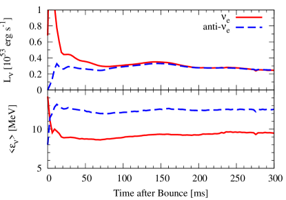
Figure 1.— Time evolution of the neutrino luminosity (top panel) and average energy (bottom panel) for $\nu_{e}$ (red-solid line) and $\bar{\nu}_{e}$ (blue-dashed line).

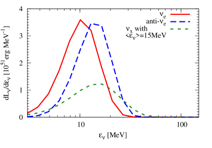
Figure 2.— The neutrino luminosity spectrum of $\nu_{e}$ (red-solid line) and $\bar{\nu}_{e}$ (blue-dashed line) without the spectral swapping at 100 ms after the bounce. For comparison, we show the injected luminosity spectrum of $\nu_{x}$ with $\left<\epsilon_{\nu_{x}}\right>=15$MeV, which will be swapped with the original spectrum of $\nu_{e}$ and $\bar{\nu}_{e}$ at $\epsilon_{\nu}>$ 9 MeV for models including spectral swapping.

3.1.2 1D with spectral swapping

The investigated models with the spectral swapping are summarized in Table 1. As already mentioned, the model parameters are the neutrinosphere radius ($R_{\nu_{x}}$), the average energy of neutrinos ($\left<\epsilon_{\nu_{x}}\right>$), and the onset time of the spectral swapping ($t_{s}$). The model names include these parameters; “NH13” represents the progenitor model, “R..” represents $R_{\nu_{x}}$ in units of km, “E..” represents $\left<\epsilon_{\nu_{x}}\right>$ in MeV, “T..” represents $t_{s}$ in ms, and the last letter “S” represents 1D (spherical symmetry).

Figure 3 presents the time evolution of the mass shells for models NH13R30E12T100S and NH13R30E13T100S. The difference between these panels is the average energies of neutrinos, $\left<\epsilon_{\nu_{x}}\right>=12$ MeV for the top panel and 13 MeV for the bottom panel. The thick solid lines represent the radial position of shock waves. Regardless of a small difference of $\left<\epsilon_{\nu_{x}}\right>$, model NH13R30E13T100S shows a shock expansion after the manual spectral swapping is switched on (see the thick line in the bottom panel of Figure 3), while the stalled shock does not revive for model NH13R30E12T100S (top panel). This suggests that there is a critical condition for the successful explosion induced by the spectral swapping. In the bottom panel, the regions enclosing the mass of $M_{r}\sim 1.2M_{\odot}$ (thin black line) corresponds to the so-called mass cut, which could be interpreted as the final mass of the remnant. The fact that a clear mass cut emerges in model NH13R30E13T100S indicates that a neutron star will be left behind in this model. Such a definite mass-cut has been observed in Kitaura et al. (2006) who reported a successful neutrino-driven explosion (in 1D) for a lighter progenitor star, which is, however, difficult to realize for more massive stars in 2D (e.g., Figure 2 in Marek & Janka (2009) and Figure 1 in Suwa et al. (2010)).

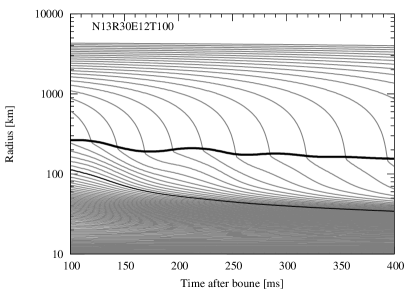
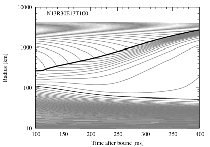
Figure 3.— Time evolution of mass shells for NH13R30E12T100S (top) and NH13R30E13T100S (bottom). The Black thin line corresponds to $1.2M_{\odot}$ and the black thick line represents the shock wave position, respectively. The difference between these panels is the average energies of neutrinos, $\left<\epsilon_{\nu_{x}}\right>=12$ MeV for the top panel and 13 MeV for the bottom panel.

As a tool to measure the strength of an explosion, we define a diagnostic energy that refers to

$$E_{\mathrm{diag}}=\int_{D}dV\left(\frac{1}{2}\rho|v|^{2}+e-\rho\Phi\right),$$ (9)

where $e$ is internal energy, $D$ represents the domain in which the integrand is positive. Figure 4 shows the time evolution of $E_{\mathrm{diag}}$ for some selected models. The diagnostic energy increases with time for the green-dotted line, which turns to decrease for the red line, noting that the difference between the pair of models is $\Delta\left<\epsilon_{\nu_{x}}\right>=1$ MeV. The blue-dashed line (model NH13R30E15T100S) has $\left<\epsilon_{\nu_{x}}\right>=15$ MeV and reaches larger $E_{\mathrm{diag}}$ than the green line (NH13R30E13T100S; $\left<\epsilon_{\nu_{x}}\right>=13$ MeV). On the other hand, the later injection of the spectral swapping leads to smaller $E_{\mathrm{diag}}$, i.e. the brown-dot-dashed line ($t_{s}$=200 ms) shows smaller $E_{\mathrm{diag}}$ than the blue-dashed line ($t_{s}=$100 ms). For models that experience earlier spectral swapping with higher neutrino energy, the diagnostic energy becomes higher in an earlier stage, as it is expected.

Looking at Figure 4 again, $E_{\mathrm{diag}}$ for the exploding models seems to show a saturation with time. These curves can be fitted by the following function,

$$E_{\mathrm{diag}}(t)=E_{\mathrm{diag}}^{\infty}(1-\mathrm{e}^{-at+b}),$$ (10)

where $E_{\mathrm{diag}}^{\infty}$ is a converging value of $E_{\mathrm{diag}}$, $a$ and $b$ are the fitting parameters. As for NH13R30E13T100S, $E_{\mathrm{diag}}^{\infty}=8.5\times 10^{50}$ erg. This fitting formula allows us to estimate the final diagnostic energy especially for the strongly exploding models whose diagnostic energy we cannot estimate in principle because the shock goes beyond the computational domains ($r<5000$ km) before the saturation.

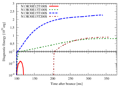
Figure 4.— Diagnostic energies as functions of time. Red-solid, green-dotted, blue-dashed and brown-dot-dashed lines correspond to models NH13R30E12T100S, NH13R30E13T100S, NH13R30E15T100S, and NH13R30E15T200S, respectively. The $\nu_{x}$ average energies of three lines other than brown-dot-dashed line differ from each other, i.e. $\left<\epsilon_{\nu_{x}}\right>=$ 12 MeV (red solid), 13 MeV (green dotted), and 15 MeV (blue dashed), respectively. As for the brown-dot-dashed line, only the onset time of spectral swapping is different from the blue-dashed line. The red-solid line shows only an oscillation, while the other lines show increasing diagnostic energy.

Figure 5 shows the summary of 1D models. For a given neutrino luminosity that is determined by $R_{\nu_{x}}$ and $\left<\epsilon_{\nu_{x}}\right>$ (equation (8)). The gray lines correspond to the neutrino luminosities determined by the pairs of $R_{\nu_{x}}$ and $\left<\epsilon_{\nu_{x}}\right>$ which is 1 to $5\times 10^{52}$ erg s^-1 from bottom to top lines. Circles and crosses correspond to the exploding and non-exploding models, respectively. Not surprisingly, explosions are more easier to be obtained for higher neutrino luminosity.

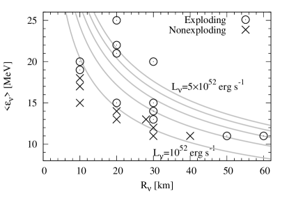
Figure 5.— Summary of 1D models with $t_{s}=100$ ms after the bounce. Circles indicate the exploding models, while crosses show non-exploding models. Gray solid lines correspond to the luminosity of $\nu_{x}$ calculated by Eq. (8), which are 1, 2, 3, 4, and $5\times 10^{52}$ erg s^-1 from bottom to top.

As is well known, the combination of $\left<\epsilon_{\nu_{x}}\right>$ and $L_{\nu_{x}}$ is an important quantity to diagnose the success or failure of explosions, because the neutrino heating rate in the so-called gain region, $Q_{\nu}^{+}$, is proportional to $\left<\epsilon_{\nu_{x}}^{2}\right>L_{\nu_{x}}$ (e.g., equation (23) in Janka (2001)).

Figure 6 shows $E_{\mathrm{diag}}^{\infty}$ as a function of $\left<\epsilon_{\nu_{x}}\right>^{2}L_{\nu_{x}}$. Note in the plot that we set the horizontal axis not as $\left<\epsilon_{\nu_{x}}^{2}\right>L_{\nu_{x}}$ but as $\left<\epsilon_{\nu_{x}}\right>^{2}L_{\nu_{x}}$ so that we can deduce the following dependence more clearly and easily. In this figure, let us first focus on red pluses, green crosses, and blue squares whose difference is characterized by $t_{s}$ (2D results (filled circles) will be mentioned in the later section). Red ($t_{s}=$100 ms), green ($t_{s}=$150 ms), and blue ($t_{s}=$200 ms) points have a clear correlation with $\left<\epsilon_{\nu_{x}}\right>^{2}L_{\nu_{x}}$. Orange and light-blue regions represent the non-exploding regions for red and blue points, respectively. Both of them show that the minimum $E_{\mathrm{diag}}^{\infty}$ decreases with $t_{s}$, indicating that the critical values of $\left<\epsilon_{\nu}\right>^{2}L_{\nu}$ for explosion sharply depends on $t_{s}$. This is because the mass outside the shock wave gets smaller with time so that the minimum energy to blow up star gets smaller too. By the same reason, $E_{\mathrm{diag}}$ becomes larger as $t_{s}$ becomes smaller given the same $\left<\epsilon_{\nu_{x}}\right>^{2}L_{\nu_{x}}$. To obtain a larger $E_{\mathrm{diag}}^{\infty}$, the earlier spectral swapping is more preferential.

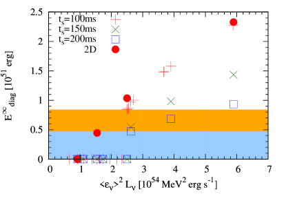
Figure 6.— Diagnostic energies for exploding models at several hundred seconds after the bounce. Red points, green crosses, and blue squares correspond to models with $t_{s}=$100, 150, and 200 ms, respectively. Red circles represent the result of 2D simulation (see text for details).

Figure 7 shows the neutrino heating rate and the density distribution of NH13R30E13T100S for 10 ms and 250 ms after $t_{s}$ (=100 ms after the bounce). As the shock wave propagates outward, the density in the gain region sharply drops (e.g., 100-200km, dashed blue line), leading to the suppression of the heating rate (dashed red line). This is the reason of the saturation in $E_{\mathrm{diag}}$ as shown in Figure 4.

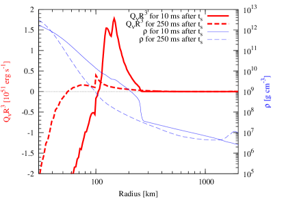
Figure 7.— Heating rate at 10 ms (red-solid line) and 250 ms (red-dashed line) after the bounce for the model NH13R30E13T100S and the density profile (blue-solid and dashed lines). As the density decreases due to the neutrino driven wind, the heating rate also decreases.

The remnant mass is an important indicator to diagnose the consequences of the explosion in producing either a neutron star or a black hole. The last two lines in Table 1 show the integrated masses in the regions of $\rho\geq 10^{10}$ g cm^-3 at $t=t_{s}$ and $t=\infty$. The latter one is estimated by the fitting as

$$M_{10}(t)=M_{10}^{\infty}(1+\mathrm{e}^{-ct+d}),$$ (11)

where $c$ and $d$ are the fitting parameters. For the exploding models, $M_{10}^{\infty}$ becomes generally smaller than $M_{10}^{t=t_{s}}$ because of the mass ejection. Exceptions are weakly exploding models (NH13R20E15T150S, NH13R20E15T200S, NH13R30E13T100S, and NH13R50E11T100S), in which the mass accretion continues after $t_{s}$ and stops eventually at late time (maximum masses are presented in Table 1). For the nonexploding models, the remnant mass simply increases with time. Regarding the 13 $M_{\odot}$ progenitor ivestigated in this section, the remnant masses in models that produce strong explosion ($E_{\mathrm{diag}}^{\infty}\gtrsim 10^{51}$ erg), are considerably smaller (1.1-1.2 $M_{\odot}$) if compared to the typical mass as of observed neutron stars $\sim 1.4M_{\odot}$ (Lattimer & Prakash, 2007). This may simply reflect the light iron core ($\sim 1.26M_{\odot}$) inherent to the progenitor or the existence of mass accretion induced by the matter fallback after the explosion. Now we move on to investigate the progenitor dependence in the next section.

Table 11D simulations

Model	Dimension	$R_{\nu}$	$\left<\epsilon_{\nu_{x}}\right>$	$L_{\nu}$	$t_{s}$	Explosion	$E_{\mathrm{diag}}^{\infty}$	$M_{10}^{t=t_{s}}$	$M_{10}^{\infty}$
		[km]	[MeV]	[1052erg s-1]	[ms]		[$10^{51}$ erg]	[$M_{\odot}$]	[$M_{\odot}$]
NH13R10E15T100S	1D	10	15MeV	0.29	100	No	—	1.18	—
NH13R10E17T100S	1D	10	17MeV	0.48	100	No	—	1.18	—
NH13R10E18T100S	1D	10	18MeV	0.60	100	No	—	1.18	—
NH13R10E19T100S	1D	10	19MeV	0.75	100	Yes	1.00	1.18	1.14
NH13R10E20T100S	1D	10	20MeV	0.92	100	Yes	1.49	1.18	1.12
NH13R20E13T100S	1D	20	13MeV	0.66	100	No	—	1.18	—
NH13R20E13T150S	1D	20	13MeV	0.66	150	No	—	1.21	—
NH13R20E13T200S	1D	20	13MeV	0.66	200	No	—	1.25	—
NH13R20E14T100S	1D	20	14MeV	0.88	100	No	—	1.18	—
NH13R20E14T150S	1D	20	14MeV	0.88	150	No	—	1.21	—
NH13R20E14T200S	1D	20	14MeV	0.88	200	No	—	1.25	—
NH13R20E15T100S	1D	20	15MeV	1.16	100	Yes	0.97	1.18	1.15
NH13R20E15T150S	1D	20	15MeV	1.16	150	Yes	0.54	1.21	$<1.24$
NH13R20E15T200S	1D	20	15MeV	1.16	200	Yes	0.47	1.25	$<1.26$
NH13R20E21T100S	1D	20	21MeV	4.47	100	Yes	5.56	1.18	1.07
NH13R20E22T100S	1D	20	22MeV	5.39	100	Yes	6.50	1.18	1.07
NH13R28E13T100S	1D	28	13MeV	1.29	100	No	—	1.18	—
NH13R29E13T100S	1D	29	13MeV	1.38	100	No	—	1.18	—
NH13R30E11T100S	1D	30	11MeV	0.76	100	No	—	1.18	—
NH13R30E11T150S	1D	30	11MeV	0.76	150	No	—	1.21	—
NH13R30E11T200S	1D	30	11MeV	0.76	200	No	—	1.25	—
NH13R30E12T100S	1D	30	12MeV	1.07	100	No	—	1.18	—
NH13R30E12T150S	1D	30	12MeV	1.07	150	No	—	1.21	—
NH13R30E12T200S	1D	30	12MeV	1.07	200	No	—	1.25	—
NH13R30E13T100S	1D	30	13MeV	1.48	100	Yes	0.85	1.18	$<1.19$
NH13R30E13T150S	1D	30	13MeV	1.48	150	No	—	1.21	—
NH13R30E13T200S	1D	30	13MeV	1.48	200	No	—	1.25	—
NH13R30E14T100S	1D	30	14MeV	1.99	100	Yes	1.58	1.18	1.12
NH13R30E14T150S	1D	30	14MeV	1.99	150	Yes	0.98	1.21	1.19
NH13R30E14T200S	1D	30	14MeV	1.99	200	Yes	0.68	1.25	1.22
NH13R30E15T100S	1D	30	15MeV	2.62	100	Yes	2.27	1.18	1.10
NH13R30E15T150S	1D	30	15MeV	2.62	150	Yes	1.43	1.21	1.16
NH13R30E15T200S	1D	30	15MeV	2.62	200	Yes	0.93	1.25	1.22
NH13R30E20T100S	1D	30	20MeV	8.28	100	Yes	6.84	1.18	1.07
NH13R40E11T100S	1D	40	11MeV	1.35	100	No	—	1.18	—
NH13R50E11T100S	1D	50	11MeV	2.10	100	Yes	0.86	1.18	$<1.18$
NH13R60E11T100S	1D	60	11MeV	3.03	100	Yes	1.48	1.18	1.12

3.1.3 The progenitor dependence

In addition to the 13 $M_{\odot}$ progenitor by Nomoto & Hashimoto (1988), we are going to investigate the progenitor dependence in 1D simulations. The computed models are NH15 ($15M_{\odot}$) (Nomoto & Hashimoto, 1988), s15s7b2 ($15M_{\odot}$) (Woosley & Weaver, 1995), s15.0 ($15M_{\odot}$), s20.0 ($20M_{\odot}$), and s25.0 ($25M_{\odot}$) (Woosley et al., 2002), which are listed in Table 2. The first sets of characters for these models indicate the progenitors as,

• NH: (Nomoto & Hashimoto, 1988)

• WW: (Woosley & Weaver, 1995)

• WHW: (Woosley et al., 2002)

Figure 8 depicts density profiles of these progenitors 100 ms after the bounce as a function of the enclosed mass ($M_{r}$). It can be seen that the density profiles for $M_{r}\lesssim 0.8M_{\odot}$ are almost insensitive to the progenitor masses despite the difference in the pre-collapse phase (see, e.g., Figure 1 of Burrows et al., 2007b). On the other hand, the profiles of $M_{r}\gtrsim 0.8M_{\odot}$ differ between progenitors so that the critical heating rates and $E_{\mathrm{diag}}^{\infty}$ are expected to be different also. In Figure 8, the envelope of WHW25 is shown to be thickest, while the envelope of NH13 is thinnest.

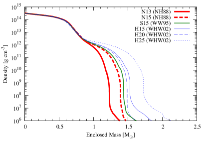
Figure 8.— Density profiles of investigated progenitors 100 ms after the bounce as functions of the enclosed mass.

Figure 9 shows the critical heating rates as a function of the progenitor masses. In agreement with intuition, the critical heating rate for models WHW25 and NH13 belongs to the high and low ends, respectively. However, the critical heating rate for model WHW20 is almost the same as the one for model NH13 although the envelope of model WHW20 is much thicker than model NH13 (see Figure 8). Our results show that the critical heating rate is indeed affected by the envelope mass, however, the relation is not one-to-one. It is also interesting to note that the critical heating rates for $15M_{\odot}$ progenitors of WW15, WHW15 and NH15, are different by a factor of $\sim 3$, which may send us a clear message that the accurate knowledge of supernova progenitors is also pivotal to pin down the supernova mechanism.

Figure 9.— The critical heating rate, $\left<\epsilon_{\nu_{x}}\right>^{2}L_{\nu_{x}}$, as a function of the progenitor mass, $M$. Circles are progenitors from Nomoto & Hashimoto (1988), the square is from Woosley & Weaver (1995), and crosses are from Woosley et al. (2002), respectively. The error bars represent the distance between the last failing and the first exploding model in our grid of models. The symbols locate at the centers of error bars. The error bar is small for model NH13 because we calculated a more refined grid of models for $13M_{\odot}$ progenitor (Table 1) than for the 15-25$M_{\odot}$ progenitors (Table 2).

The integrated masses with $\rho\geq 10^{10}$ g cm^-3 for $t=t_{s}$ and $t=\infty$ are listed in the last two lines in Table 2 and Figure 10. The tendencies are the same as found with NH13. As for model WHW25, we obtain results with $E_{\mathrm{diag}}^{\infty}>10^{51}$ erg and $M_{10}^{\infty}>1.4M_{\odot}$, simultaneously.

Figure 10.— The final NS masses as a function of the progenitor mass, $M$. Circles are progenitors from Nomoto & Hashimoto (1988), squares are from Woosley & Weaver (1995), and crosses are from Woosley et al. (2002), respectively.

Table 2Progenitor dependence

Model	Dimension	$R_{\nu}$	$\left<\epsilon_{\nu_{x}}\right>$	$L_{\nu}$	$t_{s}$	Explosion	$E_{\mathrm{diag}}^{\infty}$	$M_{10}^{t=t_{s}}$	$M_{10}^{\infty}$
		[km]	[MeV]	[1052erg s-1]	[ms]		[$10^{51}$ erg]	[$M_{\odot}$]	[$M_{\odot}$]
NH15R30E11T100S	1D	30	11MeV	0.76	100	No	—	1.34	—
NH15R30E12T100S	1D	30	12MeV	1.07	100	No	—	1.34	—
NH15R30E13T100S	1D	30	13MeV	1.48	100	Yes	0.65	1.34	$<1.38$
NH15R30E14T100S	1D	30	14MeV	1.99	100	Yes	2.17	1.34	1.25
NH15R30E15T100S	1D	30	15MeV	2.62	100	Yes	3.73	1.34	1.21
WW15R30E11T100S	1D	30	11MeV	0.76	100	No	—	1.40	—
WW15R30E12T100S	1D	30	12MeV	1.07	100	No	—	1.40	—
WW15R30E13T100S	1D	30	13MeV	1.48	100	No	—	1.40	—
WW15R30E14T100S	1D	30	14MeV	1.99	100	Yes	1.94	1.40	1.31
WW15R30E15T100S	1D	30	15MeV	2.62	100	Yes	3.41	1.40	1.25
WHW15R30E11T100S	1D	30	11MeV	0.76	100	No	—	1.49	—
WHW15R30E12T100S	1D	30	12MeV	1.07	100	No	—	1.49	—
WHW15R30E13T100S	1D	30	13MeV	1.48	100	No	—	1.49	—
WHW15R30E14T100S	1D	30	14MeV	1.99	100	No	—	1.49	—
WHW15R30E15T100S	1D	30	15MeV	2.62	100	Yes	3.55	1.49	1.36
WHW20R30E11T100S	1D	30	11MeV	0.76	100	No	—	1.45	—
WHW20R30E12T100S	1D	30	12MeV	1.07	100	No	—	1.45	—
WHW20R30E13T100S	1D	30	13MeV	1.48	100	Yes	0.99	1.45	—
WHW20R30E14T100S	1D	30	14MeV	1.99	100	Yes	2.20	1.45	1.34
WHW20R30E15T100S	1D	30	15MeV	2.62	100	Yes	3.61	1.45	1.29
WHW25R30E12T100S	1D	30	12MeV	1.07	100	No	—	1.69	—
WHW25R30E13T100S	1D	30	13MeV	1.48	100	No	—	1.69	—
WHW25R30E14T100S	1D	30	14MeV	1.99	100	No	—	1.69	—
WHW25R30E15T100S	1D	30	15MeV	2.62	100	Yes	0.73	1.69	$<2.00$
WHW25R30E16T100S	1D	30	16MeV	3.39	100	Yes	5.92	1.69	1.49
WHW25R30E17T100S	1D	30	17MeV	4.32	100	Yes	9.21	1.69	1.41

3.2. Two-dimensional models

Here we discuss the effects of spectral swapping in 2D (axisymmetric) simulations. Since our 2D simulations, albeit utilizing the IDSA scheme, are still computationally expensive, it is not practicable to perform a systematic survey in 2D as we have done in 1D simulations. Looking at Figure 9 again, we choose models WHW15 (Woosley et al., 2002) and NH13 (Nomoto & Hashimoto, 1988), whose critical heating rate belong to the high and low ends, respectively.

3.2.1 2D without spectral swapping

The basic hydrodynamic picture is the same with 1D before the shock-stall (e.g., till $\lesssim 10$ ms after bounce). After that, convection as well as SASI sets in between the stalled shock and the gain radius, which leads to the neutrino-heated shock revival for model NH13 (e.g., Suwa et al. (2010)). While for model WHW15, the position of the stalled shock, following several oscillations, begins to shrink at $\gtrsim 400$ ms after bounce.

Even after the shock revival, it should be emphasized that the shock propagation for model NH13 is the so-called “passive” one (Buras et al., 2006). This means that the amount of the mass ejection is smaller than the accretion in the post-shock region of the expanding shock (see motions of mass shells in the post-shock region of Figure 1 in Suwa et al. (2010)). Some regions have a positive local energy (Eq. (9)), but the volume integrated value is quite as small as $\lesssim 10^{50}$ erg at the maximum. In order to reverse the passive shock into an active one it is most important to energize the explosion in some way. Using these two progenitors that produce a very weak explosion (model NH13) and do not show even a shock revival (model WHW15), we hope to explore how the dynamics would change when the spectral swapping is switched on.

3.2.2 2D with spectral swapping

Table 3 shows a summary for our 2D models, in which the last character of each model (A) indicates “Axisymmetry”. Models NH13A and WHW15A are 2D models without spectral swapping for NH13 and WHW15, respectively.

As in 1D, the onset of the spectral swapping is taken to be $t_{s}=100$ ms after bounce. At this time, model NH13 shows the onset of the gradual shock expansion with a small diagnostic energy of $E_{\mathrm{diag}}\sim 3\times 10^{49}$ erg, and the shock radius is located at $\sim 300$ km. As for model WHW15, there is no region with a positive local energy (e.g., Eq. (9)) and the shock radius is $\sim 200$ km. The density profile for this model is essentially same as the one in the 1D counterpart (see Figure 8) but with small angular density modulations due to convection.

In Figure 6, red filled circles represent $E_{\mathrm{diag}}^{\infty}$ for model NH13. It can be seen that the critical heating rate to obtain $E_{\mathrm{diag}}^{\infty}\sim 10^{51}$ erg is smaller for 2D than the corresponding 1D counterparts (compare the heating rates for $\left<\epsilon_{\nu_{x}}\right>^{2}L_{\nu_{x}}\sim 2.2\times 10^{54}~{}\mathrm{MeV^{2}~{}erg~{}s^{-1}}$). In fact, models with $\left<\epsilon_{\nu_{x}}\right>^{2}L_{\nu_{x}}\lesssim 2.2\times 10^{54}~{}\mathrm{MeV^{2}~{}erg~{}s^{-1}}$ fail to explode in 1D, but succeed in 2D (albeit with a relatively small $E_{\mathrm{diag}}^{\infty}$ less than $10^{51}$ erg). As opposed to 1D, it is rather difficult in 2D to determine a critical heating rate due to the stochastic nature of the explosion triggered by SASI and convection. In our limited set of 2D models, the critical heating rate is expected to be close to $\left<\epsilon_{\nu_{x}}\right>^{2}L_{\nu_{x}}\sim 1.5\times 10^{54}~{}\mathrm{MeV^{2}~{}erg~{}s^{-1}}$, below which the shock does not revive (e.g., $\left<\epsilon_{\nu_{x}}\right>^{2}L_{\nu_{x}}\lesssim 1\times 10^{54}~{}\mathrm{MeV^{2}~{}erg~{}s^{-1}}$, is the lowest end in the horizontal axis in the figure).

As seen from Figure 6, $E_{\mathrm{diag}}^{\infty}$ becomes visibly larger for 2D than 1D especially for a smaller $\left<\epsilon_{\nu_{x}}\right>^{2}L_{\nu_{x}}$. As the heating rates become larger, the difference between 1D and 2D becomes smaller because the shock revival occurs almost in a spherically symmetric way (before SASI and convection develop non-linearly). In Table 3, it is interesting to note that model NH13R30E11T100A fails to explode, while we observed the shock-revival for the corresponding model without the spectral swapping (model NH13A). This is because the heating rate of model NH13R30E11T100A is smaller than NH13A due to the small $\left<\epsilon_{\nu_{x}}\right>$, which can make it more difficult to trigger $\nu_{x}$ explosions. On the other hand, if the energy gain due to the swap is high enough (i.e., for models with greater than E12 in Table 3), the swap can facilitate explosions.

Figure 11 depicts the entropy distributions for models NH13A (top panel) and NH13R30E13T100A (bottom panel). It can be seen that model NH13A shows a unipolar-like explosion (see also Suwa et al., 2010), while model NH13R30E13A explodes rather in a spherical manner as mentioned above. Model NH13A experiences several oscillations aided by SASI and convection before explosion, while the stalled shock for model NH13R30E13T100A, turns into expansion shortly after the onset of the spectral swapping. In fact, the shapes of hot bubbles behind the expanding shock are shown to be barely changing with time (bottom panel), which indicates a quasi-homologous expansion of material behind the revived shock.

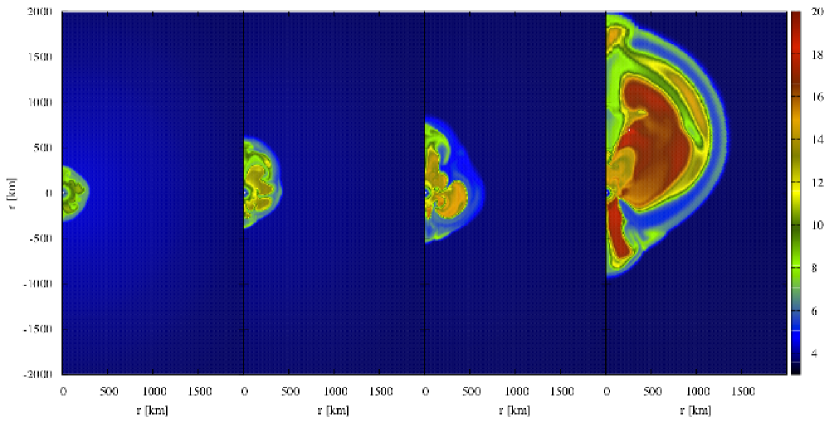
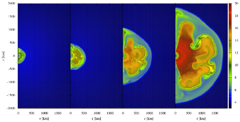
Figure 11.— Time evolution of the entropy distributions. Top: NH13A without the spectral swapping for 100, 200, 300, and 450 ms after bounce from left to right. Bottom: NH13R30E13T100A for 100, 150, 200, 250 ms after bounce (corresponding to 0, 50, 100, 150 ms after the onset of the spectral swapping.)

Figure 12 shows the time evolution of mass shells for models NH13A (thin-gray lines) and NH13R30E13T100A (thin-orange lines). Black and red thick lines represent the shock position at the north pole for each models. The mass shells for model NH13A continue to accrete to the PNS, since the shock passively expands outwards as already mentioned. Due to this continuing mass accretion, the remnant for this model would be a black hole instead of a neutron star. On the other hand, model NH13R30E13T100A shows a mass ejection with a definite outgoing momentum in the postshock region so that the remnant could be a neutron star. Unfortunately however, we cannot predict the final outcome due to the limited simulation time. A long-term simulation recently done in 1D (e.g., Fischer et al. (2010)) should be indispensable also for our 2D case. This is, however, beyond the scope of this paper.

Here let us discuss a validity of the parameters for the spectral swap that we have assumed so far. For example, the criteria of explosion for model NH13R30E12T100A was $L_{\nu_{x}}\approx 1.07\times 10^{51}$erg s^-1 and $\left<\epsilon_{\nu_{x}}\right>\approx 12$ MeV. These values are even smaller than the typical values obtained in 1D Boltzmann simulations (e.g., Liebendörfer et al. (2004)), which show $L_{\nu_{x}}\approx 2\times 10^{52}$ erg s^-1 and $\sqrt{\left<\epsilon_{\nu_{x}}^{2}\right>}\approx 20$ MeV (i.e. $\left<\epsilon_{\nu_{x}}\right>\approx 14$ MeV with a vanishing chemical potential) earlier in the postbounce phase. Therefore the spectral swapping, if it would work as we have assumed, may be a potential to assist explosions.

It should be noted that the critical heating rate in this study might be too small due to the approximation of the light-bulb scheme. In this scheme, we can include the geometrical effect of the finite size of the neturinosphere as in Eq. (7), but can not include the back reaction by the matter, i.e. the absorption of neutrino. Some fraction of neutrinos, in fact, are absorbed in the gain region and the neutrino luminosity decreases with the radius. We omit this effect in this study so that the heating rate might be overestimated in the simulation with the spectral swapping. Thus, the fully consistent simulation including the spectral swapping is necessary for more realistic critical heating rate, which is beyond the scope of this study.

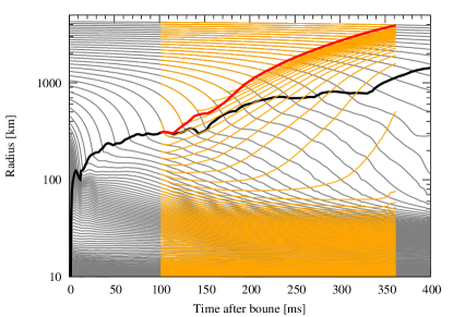
Figure 12.— Time evolution of mass shells for NH13A (thin-gray lines) and NH13R30E13T100A (thin-orange lines). Black and red thick lines represent the shock position at the north pole.

Finally we discuss the 15 $M_{\odot}$ progenitor labeled by WHW15. As mentioned, this progenitor fails to explode without spectral swapping even in 2D. Figure 13 shows the entropy distributions of WHW15A (left; nonexploding) and WHW15R30E15T100A (right; exploding) for 220 ms after the bounce (corresponding to 120 ms after $t_{s}$ for model WHW15R30E15T100A). The model with $R_{\nu_{x}}=30$ km and $\left<\epsilon_{\nu_{x}}\right>=14$ MeV does not explode in 1D but explodes in 2D (compare Table 2 and 3). Again, the mulitidimensionality helps the onset of explosion. The critical heating rate in 2D is in the range of $2.5\leq\left<\epsilon_{\nu_{x}}\right>^{2}L_{\nu_{x}}/(10^{54}$ MeV² erg s${}^{-1})\leq 3.9$, while it is $3.9\leq\left<\epsilon_{\nu_{x}}\right>^{2}L_{\nu_{x}}/(10^{54}$ MeV² erg s${}^{-1})\leq 5.9$ in 1D. Therefore the critical heating rate in 2D can be by a factor $\sim 2$ smaller than in 1D. In 2D, a critical $\nu_{x}$ luminosity and average energy to obtain explosion are $L_{\nu_{x}}\sim 2\times 10^{52}$ erg s^-1 and $\left<\epsilon_{\nu_{x}}\right>\sim 14$ MeV (corresponding to $\sqrt{\left<\epsilon_{\nu_{x}}^{2}\right>}\sim 20$ MeV), which are close to the results obtained in a 1D Boltzmann simulation (Sumiyoshi et al., 2005) for a 15 $M_{\odot}$ progenitor. The diagnostic energy as well as the estimated remnant masses are listed in the last three columns in Table 3. $E_{\mathrm{diag}}^{\infty}$ (as well as $M_{\mathrm{diag}}^{\infty}$) for exploding models is shown to be larger than the model series of NH13. As a result, some of the 2D models for WHW15 produce strong explosions ($E_{\mathrm{diag}}^{\infty}\sim 10^{51}$ erg), while simultaneously leaving behind a remnant of 1.34–1.52 $M_{\sun}$. We think that it is only a solution accidentally found by our parametric explosion models. However again, the critical heating rates that require to assist the neutrino-driven explosion via the spectral swapping are never far away from the ones obtained in the Boltzmann simulations. We hope that our exploratory results may give a momentum to supernova theorists to elucidate the effects of collective neutrino oscillations in a more consistent manner.

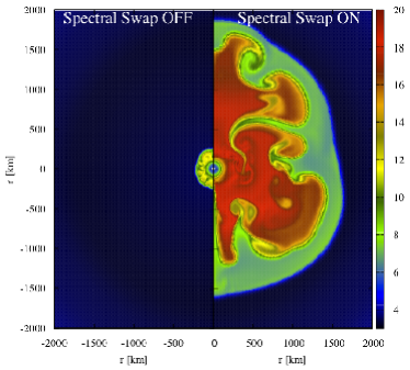
Figure 13.— The entropy distributions of WHW15A (left) and WHW15R30E15T100A (right) for 220 ms after the bounce.

Table 32D simulations

Model	Dimension	$R_{\nu}$	$\left<\epsilon_{\nu_{x}}\right>$	$L_{\nu}$	$t_{s}$	Explosion	$E_{\mathrm{diag}}^{\infty}$	$M_{10}^{t=t_{s}}$	$M_{10}^{\infty}$
		[km]	[MeV]	[1052erg s-1]	[ms]		[$10^{51}$ erg]	[$M_{\odot}$]	[$M_{\odot}$]
NH13A	2D	—	—	—	—	Yes	$\sim 0.1$ (oscillating)	—	—
NH13R30E11T100A	2D	30	11MeV	0.76	100	No	—	1.18	—
NH13R30E12T100A	2D	30	12MeV	1.07	100	Yes	0.45	1.18	$<1.23$
NH13R30E13T100A	2D	30	13MeV	1.48	100	Yes	1.03	1.18	$<1.18$
NH13R30E15T100A	2D	30	15MeV	2.62	100	Yes	2.33	1.18	1.10
WHW15A	2D	—	—	—	—	No	—	—	—
WHW15R30E13T100A	2D	30	13MeV	1.48	100	No	—	—	—
WHW15R30E14T100A	2D	30	14MeV	1.99	100	Yes	1.96	1.48	$<1.52$
WHW15R30E15T100A	2D	30	15MeV	2.62	100	Yes	3.79	1.48	1.34

4. Summary and Discussion

We performed a series of one- and two-dimensional hydrodynamic simulations of core-collapse supernovae with spectral neutrino transport via the IDSA scheme. To model the spectral swapping which is one of the possible outcomes of the collective neutrino oscillations, we parametrized the onset time when the spectral swap begins, the radius where the spectral swap takes place, and the threshold energy above which the spectral interchange between heavy-lepton neutrinos and electron/anti-electron neutrinos occurs. By doing so, we systematically studied the shock evolution and the matter ejection due to the neutrino heating enhanced by spectral swapping. We also investigated the progenitor dependence using a suite of progenitor models (13, 15, 20, and 25 $M_{\odot}$). With these computations, we found that there is a critical heating rate induced by the spectral swapping to trigger explosions, which differs between the progenitors. The critical heating rate is generally smaller for 2D than 1D due to the multidimensionality that enhances the neutrino heating efficiency (see also Janka & Mueller, 1996). The remnant masses can be determined by the mass ejection driven by the neutrino heating, which range in 1.1-1.5$M_{\odot}$ depending on the progenitors. For our 2D model of the $15M_{\odot}$ progenitor, we found a set of the parameters that produces an explosion with a canonical supernova energy close to $10^{51}$ erg and at the same time leaves behind a remnant mass close to $\sim 1.4M_{\odot}$. Our results suggest that collective neutrino oscillations have the potential to solve the supernova problem if they occurs. These effects should be explored in a more self-consistent manner in hydrodynamic simulations.

Here it should be noted that the simulations in this paper are only a very first step towards more realistic supernova modeling. For the neutrino transfer, we omitted the cooling of heavy lepton neutrinos and the inelastic neutrino scattering by electrons. These omissions lead to an overestimation of the diagnostic energy and also they should relax the criteria for explosion. The ray-by-ray approximation may lead to an overestimation of the directional dependence of the neutrino anisotropies. A full-angle transport will give us a more correct answer (see Ott et al., 2008; Brandt et al., 2011). Moreover, due to the coordinate symmetry axis, the SASI develops preferentially along the axis; it could thus provide a more favorable condition for the explosion. As several exploratory simulations have been done recently (e.g., Iwakami et al., 2008; Scheidegger et al., 2008; Nordhaus et al., 2010), 3D supernova models are indeed necessary also to pin down the outcomes of the spectral swapping.

Finally we briefly discuss whether the oscillation parameters taken in this paper are really valid in views of recent work whose focus is on clarifying the still-veiled nature of collective neutrino oscillations. Following Duan et al. (2010), there are at least two conditions for the onset of collective neutrino oscillations in the case of inverted neutrino mass hierarchy.

The first criteria should be satisfied in the so-called bipolar regime of the collective oscillation. In the regime, the neutrino number density should exceed the critical value,

$$n_{\bar{\nu}_{e},\rm crit} \simeq \frac{1}{(\sqrt{1+\chi}-1)^{2}}\frac{\Delta m^{2}}{\sqrt{2}G_{\mathrm{F}}\left<\epsilon_{\bar{\nu}_{e}}\right>}$$ (12)

$$\simeq 1.4\times 10^{29}\mathrm{cm^{-3}}\left(\frac{0.2}{\chi}\right)^{2}\left(\frac{15~{}\mathrm{MeV}}{\left<\epsilon_{\bar{\nu}_{e}}\right>}\right),$$

where $\chi$ is the fractional excess of neutrinos over antineutrinos, $\Delta m^{2}$ is the characteristic mass-squared splitting (a typical value of $\sim 2.4\times 10^{-3}$ eV² is employed here), and $G_{\mathrm{F}}$ is Fermi coupling constant. By using our simulation results, we can estimate $\chi$ which is often treated as a parameter (typically $\sim$0.01-0.25) so far. The following estimation is given in Esteban-Pretel et al. (2007), that is $\chi\simeq F_{\nu_{e}}/F_{\bar{\nu}_{e}}-1$ in the case of vanishing $F_{\nu_{x}}$, where $F_{\nu_{i}}$ is the number flux of $\nu_{i}$. From Figure 14, it can be seen that $\chi\sim$ 0.2-0.3 for 100-400 ms after bounce. Since the typical number density in the post-shock region ($r\sim$200-300 km) can be estimated as,

$$n_{\bar{\nu}_{e}} = \frac{L_{\bar{\nu}_{e}}}{4\pi r^{2}c\left<\epsilon_{\bar{\nu}_{e}}\right>}$$ (13)

$$\sim 1.1\times 10^{31}~{}\mathrm{cm}^{-3}\left(\frac{L_{\bar{\nu}_{e}}}{10^{52}~{}\mathrm{erg~{}s^{-1}}}\right)\left(\frac{100~{}\mathrm{km}}{r}\right)^{2}$$

$$\times \left(\frac{15~{}\mathrm{MeV}}{\left<\epsilon_{\bar{\nu}_{e}}\right>}\right),$$

therefore, the first condition is satisfied.

Figure 14.— Time evolution of $\chi=F_{\nu_{e}}/F_{\bar{\nu}_{e}}-1$, where $F_{\nu_{i}}$ is the number flux of $\nu_{i}$.

The second criteria is related to the decoherence of collective oscillations by matter. In order to overwhelm the suppression by the decohenrence, the following condition should be satisfied

$$n_{\bar{\nu}_{e},{\rm crit}}\sim n_{e},$$ (14)

where $n_{e}$ is the number density of electrons where the decoherence takes place. This is equivalent to,

$$Y_{\bar{\nu}_{e},{\rm crit}}\sim Y_{e}.$$ (15)

In our 1D simulation, $Y_{\bar{\nu}_{e}}\sim(0.1-0.2)\times Y_{e}$ for 100 km $\lesssim r\lesssim r_{\mathrm{sh}}$, where $r_{\mathrm{sh}}$ is the shock radius. Since this condition is barely satisfied, the collective oscillations in reality could modify the spectrum to some extent between heavy-lepton neutrinos and electron/anti-electron neutrinos, however the full swapping assumed in this study may be exaggerated. Very recently, Chakraborty et al. (2011a, b) pointed out that the matter effect could fully suppress the spectral swapping in the accretion phase using 1D neutrino-radiation hydrodynamic simulation data of Fischer et al. (2010). However, the current understanding of the collective oscillation is not completed and calculations in this field employ several assumptions (e.g., single angle approximation) (but see also Dasgupta et al., 2011, for more recent work). To draw a robust conclusion, one needs a more detailed study including the collective neutrino flavor oscillation to the hydrodynamic simulations in a more self-consistent manner, which we are going to challenge as a sequel of this study.

Appendix A Code Validity

A.1. Conservation of Energy

In this section, we demonstrate the conservation of physical quantities using the spherical collapse model (NH13). Figure 15 depicts the evolution of total binding energy by gravity (red line), total internal energy (green), total kinetic energy (blue), total trapped-neutrino energy (magenta), total energy leaked by neutrinos (cyan), and variation of overall energy (black dashed), respectively. The gravitational energy and total energy are negative and absolute values are shown. The gravitational energy and internal energy dominate (with different sign) and reach $\sim 10^{53}$ erg soon after bounce. Despite such an enormous energy change, the total energy varies only within $\sim 3\times 10^{49}$ erg so that the violation of energy conservation remains $<0.03\%$. The energy of the trapped neutrinos decreases with the diffusion timescale, which leads to the PNS cooling. The kinetic energy rapidly drops because of the photodissociation of iron and the electron capture ($\nu_{e}$ emission) that is consistent with the shock stall. We have monitored these values in a 2D simulation and obtained a similar level of energy conservation.

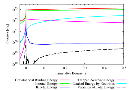
Figure 15.— Time evolution of gravitational energy (red), internal energy (green line), kinetic energy (blue line), trapped-neutrino energy (magenta line), released energy by neutrinos (cyan line), and summation of these energies (black dashed line). These quantities are determined by integration with respect to volume included in our simulation except for released energy by neutrinos (magenta), which is $\int(L_{\nu_{e}}+L_{\bar{\nu}_{e}})dt$. Since gravitational energy and total energy are negative, the absolute values are shown. The violation of total energy (dashed line) remains $<3\times 10^{49}$ erg, which is $\sim 0.03\%$ of gravitational energy and internal energy after bounce ($\sim 10^{53}$ erg).

A.2. Comparison with AGILE

Here, we present the result of our numerical simulation in spherical symmetry and compare with the result of AGILE-IDSA code (Liebendörfer et al., 2009). AGILE (Adaptive Grid with Implicit Leap Extrapolation) is an implicit general relativistic hydrodynamics code that evolves the Einstein equations based on conservative finite differencing on an adaptive grid. We employ a one-dimensional version of our ZEUS-2D code that has been developed to perform multidimensional supernova simulations.

We compare the evolution of a $13M_{\odot}$ star of Nomoto & Hashimoto (1988) in Newtonian gravity from precollapse model to 100 ms after bounce. We find good agreement between the results of the ZEUS-2D and AGILE during the early postbounce phase when the neutrino burst is launched and the accretion shock expands to its maximum radius. The hydrodynamic quantities are shown in following figures.

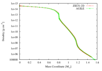
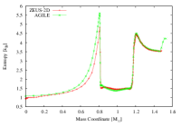
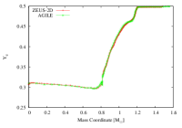
Figure 16.— Density (left top), entropy (right top), velocity (left bottom), and electron fraction (right bottom) as a function of enclosed mass for the result of ZEUS-2D (red lines) and AGILE (green lines). The comparison is shown at the time just after the bounce. A difference is seen in the entropy profile, which comes from the difference of shock capturing scheme.

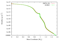
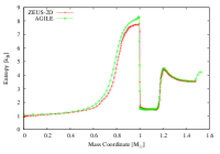
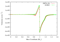
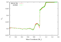
Figure 17.— Same as Fig. 16 but for the time at 1 ms after bounce.

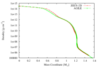
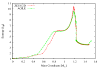
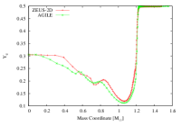
Figure 18.— Same as Fig. 16 but for the time at 100 ms after bounce.

References

- Bethe & Wilson (1985) Bethe, H. A., & Wilson, J. R. 1985, ApJ, 295, 14
- Blondin et al. (2003) Blondin, J. M., Mezzacappa, A., & DeMarino, C. 2003, ApJ, 584, 971
- Brandt et al. (2011) Brandt, T. D., Burrows, A., Ott, C. D., & Livne, E. 2011, ApJ, 728, 8
- Bruenn et al. (2009) Bruenn, S. W., Mezzacappa, A., Hix, W. R., Blondin, J. M., Marronetti, P., Messer, O. E. B., Dirk, C. J., & Yoshida, S. 2009, in American Institute of Physics Conference Series, Vol. 1111, American Institute of Physics Conference Series, ed. G. Giobbi, A. Tornambe, G. Raimondo, M. Limongi, L. A. Antonelli, N. Menci, & E. Brocato, 593–601
- Buras et al. (2006) Buras, R., Janka, H., Rampp, M., & Kifonidis, K. 2006, A&A, 457, 281
- Burrows et al. (2007a) Burrows, A., Dessart, L., Livne, E., Ott, C. D., & Murphy, J. 2007a, ApJ, 664, 416
- Burrows et al. (1995) Burrows, A., Hayes, J., & Fryxell, B. A. 1995, ApJ, 450, 830
- Burrows et al. (2007b) Burrows, A., Livne, E., Dessart, L., Ott, C. D., & Murphy, J. 2007b, ApJ, 655, 416
- Chakraborty et al. (2011a) Chakraborty, S., Fischer, T., Mirizzi, A., Saviano, N., & Tomas, R. 2011a, arXiv:1104.4031
- Chakraborty et al. (2011b) Chakraborty, S., Fischer, T., Mirizzi, A., Saviano, N., & Tomas, R. 2011b, arXiv:1105.1130
- Colgate & White (1966) Colgate, S. A., & White, R. H. 1966, ApJ, 143, 626
- Dasgupta (2010) Dasgupta, B. 2010, arXiv:1005.2681
- Dasgupta et al. (2008) Dasgupta, B., Dighe, A., & Mirizzi, A. 2008, Physical Review Letters, 101, 171801
- Dasgupta et al. (2011) Dasgupta, B., O’Connor, E. P. & Ott, C. D. 2011, arXiv:1106.1167
- Demorest et al. (2010) Demorest, P. B., Pennucci, T., Ransom, S. M., Roberts, M. S. E., & Hessels, J. W. T. 2010, Nature, 467, 1081
- Duan et al. (2008) Duan, H., Fuller, G. M., & Carlson, J. 2008, Computational Science and Discovery, 1, 015007
- Duan et al. (2010) Duan, H., Fuller, G. M., & Qian, Y. 2010, Annual Review of Nuclear and Particle Science, 60, 569
- Esteban-Pretel et al. (2007) Esteban-Pretel, A., Pastor, S., Tomàs, R., Raffelt, G. G., & Sigl, G. 2007, Phys. Rev. D, 76, 125018
- Fernández (2010) Fernández, R. 2010, ApJ, 725, 1563
- Fischer et al. (2010) Fischer, T., Whitehouse, S. C., Mezzacappa, A., Thielemann, F., & Liebendörfer, M. 2010, A&A, 517, A80+
- Fogli et al. (2007) Fogli, G., Lisi, E., Marrone, A., & Mirizzi, A. 2007, Journal of Cosmology and Astro-Particle Physics, 12, 10
- Foglizzo et al. (2007) Foglizzo, T., Galletti, P., Scheck, L., & Janka, H. 2007, ApJ, 654, 1006
- Fryer & Warren (2002) Fryer, C. L., & Warren, M. S. 2002, ApJ, 574, L65
- Fryer & Warren (2004) —. 2004, ApJ, 601, 391
- Guilet et al. (2010) Guilet, J., Sato, J., & Foglizzo, T. 2010, ApJ, 713, 1350
- Herant et al. (1994) Herant, M., Benz, W., Hix, W. R., Fryer, C. L., & Colgate, S. A. 1994, ApJ, 435, 339
- Iwakami et al. (2008) Iwakami, W., Kotake, K., Ohnishi, N., Yamada, S., & Sawada, K. 2008, ApJ, 678, 1207
- Janka (2001) Janka, H. 2001, A&A, 368, 527
- Janka & Mueller (1996) Janka, H., & Mueller, E. 1996, A&A, 306, 167
- Kitaura et al. (2006) Kitaura, F. S., Janka, H., & Hillebrandt, W. 2006, A&A, 450, 345
- Kotake et al. (2006) Kotake, K., Sato, K., & Takahashi, K. 2006, Rep. Prog. Phys., 69, 971
- Kotake et al. (2004) Kotake, K., Sawai, H., Yamada, S., & Sato, K. 2004, ApJ, 608, 391
- Langanke et al. (2003) Langanke, K., et al. 2003, Physical Review Letters, 90, 241102
- Lattimer & Prakash (2007) Lattimer, J. M., & Prakash, M. 2007, Phys. Rep., 442, 109
- Lattimer & Swesty (1991) Lattimer, J. M., & Swesty, F. D. 1991, Nuclear Physics A, 535, 331
- Liebendörfer et al. (2004) Liebendörfer, M., Messer, O. E. B., Mezzacappa, A., Bruenn, S. W., Cardall, C. Y., & Thielemann, F. 2004, ApJS, 150, 263
- Liebendörfer et al. (2001) Liebendörfer, M., Mezzacappa, A., Thielemann, F.-K., Messer, O. E., Hix, W. R., & Bruenn, S. W. 2001, Phys. Rev. D, 63, 103004
- Liebendörfer et al. (2009) Liebendörfer, M., Whitehouse, S. C., & Fischer, T. 2009, ApJ, 698, 1174
- Marek & Janka (2009) Marek, A., & Janka, H. 2009, ApJ, 694, 664
- Masada et al. (2011) Masada, Y., Takiwaki, T., & Kotake, K. 2011, submitted to ApJ
- Müller et al. (2010) Müller, B., Janka, H., & Dimmelmeier, H. 2010, ApJS, 189, 104
- Murphy & Burrows (2008) Murphy, J. W., & Burrows, A. 2008, ApJ, 688, 1159
- Nomoto & Hashimoto (1988) Nomoto, K., & Hashimoto, M. 1988, Phys. Rep., 163, 13
- Nordhaus et al. (2010) Nordhaus, J., Burrows, A., Almgren, A., & Bell, J. 2010, ApJ, 720, 694
- Obergaulinger et al. (2006) Obergaulinger, M., Aloy, M. A., & Müller, E. 2006, A&A, 450, 1107
- Obergaulinger & Janka (2011) Obergaulinger, M., & Janka, H.-T. 2011, arXiv:1101.1198
- O’Connor & Ott (2011) O’Connor, E., & Ott, C. D. 2011, ApJ, 730, 70
- Ohnishi et al. (2006) Ohnishi, N., Kotake, K., & Yamada, S. 2006, ApJ, 641, 1018
- Ott et al. (2008) Ott, C. D., Burrows, A., Dessart, L., & Livne, E. 2008, ApJ, 685, 1069
- Raffelt & Smirnov (2007) Raffelt, G. G., & Smirnov, A. Y. 2007, Phys. Rev. D, 76, 081301
- Rampp & Janka (2002) Rampp, M., & Janka, H. 2002, A&A, 396, 361
- Sagert et al. (2009) Sagert, I., Fischer, T., Hempel, M., Pagliara, G., Schaffner-Bielich, J., Mezzacappa, A., Thielemann, F., & Liebendörfer, M. 2009, Physical Review Letters, 102, 081101
- Scheck et al. (2006) Scheck, L., Kifonidis, K., Janka, H., & Müller, E. 2006, A&A, 457, 963
- Scheidegger et al. (2008) Scheidegger, S., Fischer, T., Whitehouse, S. C., & Liebendörfer, M. 2008, A&A, 490, 231
- Shlomo et al. (2006) Shlomo, S., Kolomietz, V. M., & Colò, G. 2006, European Physical Journal A, 30, 23
- Stone & Norman (1992) Stone, J. M., & Norman, M. L. 1992, ApJS, 80, 753
- Strack & Burrows (2005) Strack, P., & Burrows, A. 2005, Phys. Rev. D, 71, 093004
- Sumiyoshi et al. (2005) Sumiyoshi, K., Yamada, S., Suzuki, H., Shen, H., Chiba, S., & Toki, H. 2005, ApJ, 629, 922
- Suwa et al. (2010) Suwa, Y., Kotake, K., Takiwaki, T., Whitehouse, S. C., Liebendörfer, M., & Sato, K. 2010, PASJ, 62, L49
- Suwa et al. (2007a) Suwa, Y., Takiwaki, T., Kotake, K., & Sato, K. 2007a, ApJ, 665, L43
- Suwa et al. (2007b) —. 2007b, PASJ, 59, 771
- Suwa et al. (2009) —. 2009, ApJ, 690, 913
- Suzuki et al. (2008) Suzuki, T. K., Sumiyoshi, K., & Yamada, S. 2008, ApJ, 678, 1200
- Takiwaki et al. (2009) Takiwaki, T., Kotake, K., & Sato, K. 2009, ApJ, 691, 1360
- Thompson et al. (2003) Thompson, T. A., Burrows, A., & Pinto, P. A. 2003, ApJ, 592, 434
- Thompson et al. (2005) Thompson, T. A., Quataert, E., & Burrows, A. 2005, ApJ, 620, 861
- Woosley et al. (2002) Woosley, S. E., Heger, A., & Weaver, T. A. 2002, Reviews of Modern Physics, 74, 1015
- Woosley & Weaver (1995) Woosley, S. E., & Weaver, T. A. 1995, ApJS, 101, 181
- Yakunin et al. (2010) Yakunin, K. N., et al. 2010, Classical and Quantum Gravity, 27, 194005
- Yamada (2000) Yamada, S. 2000, Phys. Rev. D, 62, 093026