Dijet Invariant Mass Distribution in Top Quark Hadronic Decay with QCD Corrections

Abstract

The dijet invariant mass distributions from the hadronic decay of unpolarized top quark ($t\to bW^{+}$ followed by $W^{+}\to u\bar{d}$) are calculated, including the next-to-leading order QCD radiative corrections. We treat the top decay in the complex mass scheme due to the existence of the intermediate state W boson. Our analytical expressions are also available in different dimensional regularization schemes and $\gamma_{5}$ strategies. Finally, in order to construct the jets, we use different jet algorithms to compare their influences on our results. The obtained dijet mass distributions from the top quark decay are useful to distinguish these dijets from those produced via other sources and to clarify the issue about the recent CDF Collaborations’ $Wjj$ anomaly.

I Introduction

Since the discovery of the top quark at the TevatronAbe:1995hr ; Abachi:1995iq , the top quark has played a special role in searching for the electroweak symmetry breaking mechanism and new physics beyond the standard model. This can be attributed to the large mass of the top quark (about $173~{}{\rm GeV}$ ), which is almost 40 times larger than the next heaviest quark. As the Cabibbo-Kabayashi-Maskawa matrix element $V_{tb}$ approaches to 1, the top quark decays almost to a bottom quark and a W boson. Its decay width Harris:2002md ; Jezabek:1988iv ; Campbell:2004ch ; Schmidt:1995mr is $\mathcal{O}(GeV)$, much larger than the typical QCD scale $\Lambda_{QCD}\sim 300MeV$, indicating that the top quark decay takes place before hadronization. Therefore, nonperturbative effects are not important in the properties of the top quark, and one can perturbatively calculate its physical quantities precisely, such as top quark’s spin correlation. At the Large Hadron Collider (LHC) at CERN, thousands of top quarks are expected to be produced per year at 14 TeV. Hence a new era in top quark research has arrived.

On the other hand, very recently a dijet bump around 150 GeV in the $Wjj$ channel has been observed by the Collider Detector at Fermilab (CDF) at the TevatronAaltonen:2011mk , and it has attracted a lot of attention. There are some explanations within the standard model for this anomalyHe:2011ss ; Sullivan:2011hu ; Plehn:2011nx . Some studies may indicate that single top production may play an important role in the CDF dijet excess. Moreover, the D0 Collaboration reported that their results were consistent with the standard model’s prediction in the same channelAbazov:2011af . Hence a careful investigation regarding the dijet in the single top production and decay is helpful. Even without this CDF anomaly, it is still useful to study the dijet distribution in the top quark decay, as a part of investigations for the top quark properties. Inspired by this, in the present study we will investigate the dijet mass distribution in the top quark decay. This work also aims at understanding the properties of top quarks.

There are a lot of works already about top quark decaysDenner:1990ns ; Brandenburg:2002xr ; Liu:1990py ; Czarnecki:1990kv ; Li:1990qf ; Jezabek:1988iv ; Ghinculov:2000nx ; Eilam:1991iz ; Barroso:2000is ; Oliveira:2001vw ; Czarnecki:1998qc ; Chetyrkin:1999ju ; Fischer:1998gsa ; Fischer:2000kx ; Fischer:2001gp ; Penin:1998wj ; Jezabek:1993wk ; Do:2002ky . Generally, the QCD next-to-leading order (NLO) radiative corrections to the top quark’s width amount to about $-8.54\%$Denner:1990ns ; Liu:1990py ; Czarnecki:1990kv ; Li:1990qf ; Jezabek:1988iv ; Ghinculov:2000nx , while the corrections of QCD two loops Czarnecki:1998qc ; Chetyrkin:1999ju and electroweak one loopDenner:1990ns ; Eilam:1991iz ; Barroso:2000is are about $-2.05\%$ and $1.54\%$ respectively. The nonvanishing $m_{b}$ effects Fischer:1998gsa ; Fischer:2000kx ; Fischer:2001gp ; Penin:1998wj and finite width correctionsJezabek:1993wk reduce the Born level width by about $0.27\%$ and $1.55\%$. All these show that the QCD NLO corrections, among others, are important for top quarks. Therefore, in the present study, we also put stress on the effects of QCD NLO corrections to the dijet distributions in the top quark decay.

The rest of the paper is organized as follows. Section II demonstrates the dimensional regularization schemes and $\gamma_{5}$ schemes. Section III tackles our scheme-independent analytical expressions. Jet algorithms are recalled in Sec. IV and Sec. V discusses the results. The final section contains the conclusion.

II Dimensional Regularization Schemes And $\gamma_{5}$ Schemes

Dimensional regularization has many advantages in dealing with ultraviolet, infrared and mass divergences encountered in high-order calculations in a unified manner. However, there are still some freedoms to handle these divergences in dimensional regularization. In this section we recall four modern versions of frequently used schemes and adopt the first three in the rest of this paper. The four schemes include the conventional dimensional regularization (CDR), the ’t-Hooft-Veltman scheme (HV)'tHooft:1972fi , the four dimensional helicity scheme (FDH)Bern:2002zk ; Kunszt:1993sd ; Bern:1991aq ; Bern:1994zx ; Bern:1994cg , and the dimensional reduction scheme (DR)Siegel:1979wq .

In CDR, only the $d=4-2\epsilon$ dimensional metric tensor is introduced, i.e. $g^{\mu}_{\mu}=d$. The loop momentum and the spins of vectors, regardless of whether they are ”observed” or ”unobserved” are in $d$ dimensions, whereas the spins of the spinor are in $d_{s}$ dimensions with $d_{s}\geq d$. In this section, the observed states refer to the external states appearing in the hard part of the process without any subsequent hadronization. We treat $d_{s}$ of fermions as four because it is distinct from $d$ and always appears as a global factor in computations.

HV and FDH have many advantages in helicity amplitude calculations, while FDH and DR are two supersymmmetric preserving schemesSiegel:1979wq ; Kunszt:1993sd ; Bern:1994zx ; Bern:1994cg . We describe the schemes in a unified way as explained below:

• To maintain the gauge invariance, all momentum integrals are integrated in $d$ dimensions.

• The dimensions of all observed particles (hard and noncollinear external particles) are left in four dimensions.

• The dimensions of all unobserved particles (internal states and soft or collinear external states ) are treated in $d_{s}$ dimensions . Any explicit factors of dimension arising from these state should be labeled as $d_{s}$ temporary; these must be kept distinct from $d$ at the beginning.

We treat internal states with $d>4$ in HV and FDH, whereas $d<4$ in DR, i.e., all variables in $d$ dimensions can be divided into a four-dimensional part and $d-4$-dimensional part in CDR, HV and FDH, while a four-dimensional quantity can be split into $d$ and $4-d$-dimensional quantities in DR. The expressions are analytic functions of $d$ and they are continued to any desired regions. Setting $d_{s}=d$ denoted in the above items, we obtain the HV scheme, while setting $d_{s}=4$ results in the FDH and DR schemes. As mentioned above, the $d_{s}$ arising from dimensions of spinor space is just a global factor. Therefore, we can set this part of $d_{s}$ to be equal to 4. All of the above is summarized in Table 1.

Table 1: Summary of dimensions in different regularization schemes.

Regularization schemes	CDR	HV	FDH	DR
Dimensions of momenta of observed particles	$d$	$4$	$4$	$4$
Dimensions of momenta of unobserved particles	$d$	$d$	$d$	$d$
Number of polarizations of observed massless vector bosons	$d-2$	$2$	$2$	$2$
Number of polarizations of unobserved massless vector bosons	$d-2$	$d-2$	$2$	$2$
Number of polarizations of observed massive vector bosons	$d-1$	$3$	$3$	$3$
Number of polarizations of unobserved massive vector bosons	$d-1$	$d-1$	$3$	$3$
Number of polarizations of fermions	$2$	$2$	$2$	$2$

Dimensional regularization has algebraic consistency problems with respect to $\gamma_{5}$. $\gamma_{5}=\frac{i}{4}\varepsilon_{\mu\nu\rho\sigma}\gamma^{\mu}\gamma^{\nu}\gamma^{\rho}\gamma^{\sigma}$, which is well defined in four dimensions. However, there are some problems with this definition because antisymmetric tensor $\varepsilon_{\mu\nu\rho\sigma}$ lives in four dimensions only. In the naive definition of $\gamma_{5}$, some obviously inconsistent equalities appear. If we keep all the four-dimensional rules and cyclicity of the trace, the analytic continuation is forbiddenKreimer:1989ke . Therefore, one should at least change one of the properties to obtain a consistent result. To the best of our knowledge, there are two kinds of well-known $\gamma_{5}$ strategies that have been introduced; one is proposed by ’t-Hooft and Veltman and proved by Breitenlohner and Maison Breitenlohner:1977hr ; Breitenlohner:1975hg ; Breitenlohner:1976te ; 'tHooft:1972fi (we call it the BMHV scheme), and the other one is introduced by Korner, Kreimer and Schilcher Kreimer:1993bh ; Korner:1991sx ; Kreimer:1989ke (we call it the KKS scheme).

As a compromise, in the BMHV scheme the anticommutation relationship between $\gamma_{5}$ and $\gamma_{\mu}$ is violated, i.e. $\{\gamma_{5},\gamma_{\mu}\}\neq 0$. In fact, every $d$-dimensional quantity can be divided into a four-dimensional part and a $-2\varepsilon$ part, which implies that in this scheme $d>4$. $\gamma_{5}$ anticommutes with a four-dimensional $\gamma$-matrix, while it commutes with a $-2\varepsilon$-dimensional $\gamma$-matrix. This definition results in some ambiguousness of chiral vector current treatment, e.g. $\gamma^{\mu}\frac{1\pm\gamma_{5}}{2}\neq\frac{1\mp\gamma_{5}}{2}\gamma^{\mu}$ in tree-level Feynman rules. For the current work, we take the symmetric version as presented in Korner:1989is ; Buras:1998raa , i.e.

$$\gamma^{\mu}\frac{1-\gamma_{5}}{2} \rightarrow \frac{1+\gamma_{5}}{2}\gamma^{\mu}\frac{1-\gamma_{5}}{2},$$

$$\gamma^{\mu}\frac{1+\gamma_{5}}{2} \rightarrow -\frac{1+\gamma_{5}}{2}\gamma^{\mu}\frac{1-\gamma_{5}}{2}+\gamma^{\mu}.$$ (1)

The violation of anticommutation is also a violation of the Ward identity in axial-vector currents. To prevent such a violation, additional renormalization is neededHarris:2002md (Readers who are interested in dimensional renormalization issues can also refer to Refs.Martin:1999cc ; Schubert:1988ke ; Pernici:1999nw ; Pernici:1999ga ; Pernici:2000an ; Ferrari:1994ct ). This will be used in the next section. Although it is the first rigorously proven consistent scheme, the process of isolating four-dimensional and $-2\varepsilon$ parts in the Lorentz space often suffers from complex practical calculations.

On all accounts, the strategy of covariance violation in $\gamma_{5}$ has some disadvantages in complicated situations. On the other hand, the KKS scheme keeps the covariant anticommutations but forbids the cyclicity in the trace. In $\gamma$-matrix algebra (Clifford algebra), there is a unique generator, which anticommutes with all other generators in infinite dimensions. This generator can be defined as the $\gamma_{5}$. To avoid the cyclicity in the trace, the ”reading point” must be chosen first, and all $\gamma_{5}$ are moved to this point before a trace is taken. This compromise recovers a correct anomaly as well.

Finally, we also introduce the renormalization constants and the splitting functions in the CDR, HV, and FDH dimensional regularization schemes used in this paper. In order to avoid calculating external self energy diagrams, we choose the on-shell scheme for external legs. These constants are

$$\delta Z^{OS}_{t} = -\frac{\alpha_{s}C_{F}}{4\pi}\left(\frac{1}{\epsilon_{UV}}+\frac{2}{\epsilon_{IR}}-3\gamma_{E}+3\ln\left(\frac{4\pi\mu^{2}}{m_{t}^{2}}\right)+4+1_{FDH}\right),$$

$$\delta Z^{OS}_{q} = -\frac{\alpha_{s}C_{F}}{4\pi}\left(\frac{1}{\epsilon_{UV}}-\frac{1}{\epsilon_{IR}}\right),$$ (2)

where $\delta Z^{OS}_{t}$, $\delta Z^{OS}_{q}$ are on-shell(OS) wave function renormalization constants for top quark and light quarks, respectively, $\gamma_{E}$ is the Euler constant, and $1_{FDH}$ is only nonvanishing in FDH scheme. The unpolarized Altarelli-Parisi splitting functions Altarelli:1977zs ; Catani:1996pk to $\mathcal{O}(\epsilon)$ in HV and CDR schemes are all listed in the following:

$$P_{qq}(z) = C_{F}\frac{1+z^{2}}{1-z}-\epsilon~{}C_{F}(1-z),$$

$$P_{gq}(z) = C_{F}\frac{1+(1-z)^{2}}{z}-\epsilon~{}C_{F}~{}z,$$

$$P_{gg}(z) = 2N_{c}\left(\frac{z}{1-z}+\frac{1-z}{z}+z(1-z)\right),$$

$$P_{qg}(z) = \frac{z^{2}+(1-z)^{2}}{2}-\epsilon~{}z(1-z),$$ (3)

while in FDH and DR these terms should be

$$P_{qq}(z) = C_{F}\frac{1+z^{2}}{1-z},$$

$$P_{gq}(z) = C_{F}\frac{1+(1-z)^{2}}{z},$$

$$P_{gg}(z) = 2N_{c}\left(\frac{z}{1-z}+\frac{1-z}{z}+z(1-z)\right)+\epsilon~{}2N_{c}~{}z(1-z),$$

$$P_{qg}(z) = \frac{z^{2}+(1-z)^{2}}{2}-\epsilon~{}z(1-z).$$ (4)

III Scheme Independence And Analytical Expressions

As emphasized in Sec.II, there are some degrees of freedom to regularize possible divergences. Because of unitarity in QCD cross sectionsCatani:1996pk , we should expect the scheme independence of the well-defined physical results. In this section, analytical results are provided for top quark decay and subsequent hadronic decay, thus affirming the simplicity of these processes. Moreover, we also demonstrate that the off-shell effect in the top quark hadronic decay is small, and narrow-width-approximation is good enough at the decay width level.

III.1 Corrections To $t\rightarrow bW^{+}$

We first reproduce the well-known QCD corrections to the top quark decayHarris:2002md ; Jezabek:1988iv ; Campbell:2004ch ; Schmidt:1995mr (Feynman diagrams generated by FEYNARTS Hahn:2000kx are shown in Fig.1). Because of the Cabibbo-Kabayashi-Maskawa (CKM) matrix elements $1\approx|V_{tb}|\gg|V_{ts}|,|V_{td}|$, the branching ratio of $t\rightarrow bW^{+}$ is almost $100\%$. For simplification, we set the CKM matrix to be diagonal and the mass of the b-quark equal to zero. As presented in previous works, the effect of nonvanishing mass of the bottom quark is negligible. Following the notations of Ref.Campbell:2004ch , the matrix element of the tree-level process $t(p_{t})\rightarrow b(p_{b})W^{+}(p_{W})$ with averaging over the top quark’s spin and color is given by

$$|\overline{\mathcal{M}}_{0}|^{2} = \frac{e^{2}m_{t}^{4}}{4s_{w}^{2}m_{W}^{2}}\left(1-r^{2}\right)\left(1+2r^{2}\right),$$ (5)

where $r=\frac{m_{W}}{m_{t}}$ and $s_{w}$ is the sine of Weinberg angle. We can get the leading-order width easily

$$\Gamma_{0} = \frac{\alpha m_{t}^{3}}{16s_{w}^{2}m_{w}^{2}}\left(1-r^{2}\right)^{2}\left(1+2r^{2}\right),$$ (6)

where we have used the electromagnetic fine-structure coupling constant $\alpha=\frac{e^{2}}{4\pi}$.

To check the regularization scheme independence of these results, we first derive the averaged squared matrix element in the FDH regularization scheme within the naive or KKS $\gamma_{5}$ scheme. The virtual terms and counter-terms for renormalization are given by

$$\left(|\overline{\mathcal{M}}_{v}|^{2}+|\overline{\mathcal{M}}_{ct}|^{2}\right)^{KKS}_{FDH} = |\overline{\mathcal{M}}_{0}|^{2}\frac{\alpha_{s}~{}C_{F}}{2\pi\Gamma(1-\epsilon)}\left(\frac{4\pi\mu^{2}}{m_{t}^{2}}\right)^{\epsilon}$$ (7)

$$\left[-\frac{1}{\epsilon^{2}}-\frac{\frac{5}{2}-2\ln(1-r^{2})}{\epsilon}-\frac{11}{2}-\frac{\pi^{2}}{6}+3\ln(1-r^{2})\right.$$

$$-\frac{\ln(1-r^{2})}{r^{2}}+\frac{1-r^{2}}{r^{2}(1+2r^{2})}\ln(1-r^{2})$$

$$\left.-2\ln^{2}(1-r^{2})-2~{}\text{Li}_{2}(r^{2})\right].$$

In order to see the scheme-dependent terms, we subtract the expressions in other schemes by the expressions in FDH with KKS $\gamma_{5}$ treatment and use $\delta|\overline{\mathcal{M}}_{v/ct/real}|^{2}\doteq|\overline{\mathcal{M}}_{v/ct/real}|^{2}-\left(|\overline{\mathcal{M}}_{v/ct/real}|^{2}\right)^{KKS}_{FDH}$. These scheme-dependent terms are

$$\left(\delta|\overline{\mathcal{M}}_{v}|^{2}+\delta|\overline{\mathcal{M}}_{ct}|^{2}\right)^{KKS}_{HV} = -|\overline{\mathcal{M}}_{0}|^{2}\frac{\alpha_{s}~{}C_{F}}{4\pi},$$

$$\left(\delta|\overline{\mathcal{M}}_{v}|^{2}+\delta|\overline{\mathcal{M}}_{ct}|^{2}\right)^{KKS}_{CDR} = |\overline{\mathcal{M}}_{0}|^{2}\frac{\alpha_{s}~{}C_{F}}{4\pi\Gamma(1-\epsilon)}\left(\frac{4\pi\mu^{2}}{m_{t}^{2}}\right)^{\epsilon}\frac{1}{1+2r^{2}}$$

$$\left[\frac{4r^{2}}{\epsilon}+8r^{2}-1-8r^{2}\ln(1-r^{2})\right],$$

$$\left(\delta|\overline{\mathcal{M}}_{v}|^{2}+\delta|\overline{\mathcal{M}}_{ct}|^{2}\right)^{BMHV}_{FDH} = |\overline{\mathcal{M}}_{0}|^{2}\frac{\alpha_{s}~{}C_{F}}{2\pi},$$

$$\left(\delta|\overline{\mathcal{M}}_{v}|^{2}+\delta|\overline{\mathcal{M}}_{ct}|^{2}\right)^{BMHV}_{HV} = |\overline{\mathcal{M}}_{0}|^{2}\frac{3~{}\alpha_{s}~{}C_{F}}{4\pi},$$

$$\left(\delta|\overline{\mathcal{M}}_{v}|^{2}+\delta|\overline{\mathcal{M}}_{ct}|^{2}\right)^{BMHV}_{CDR} = |\overline{\mathcal{M}}_{0}|^{2}\frac{\alpha_{s}~{}C_{F}}{4\pi\Gamma(1-\epsilon)}\left(\frac{4\pi\mu^{2}}{m_{t}^{2}}\right)^{\epsilon}\frac{1}{1+2r^{2}}$$ (8)

$$\left[\frac{4r^{2}}{\epsilon}+3+16r^{2}-8r^{2}\ln(1-r^{2})\right].$$

These scheme-dependent terms should be canceled exactly with real corrections originated from soft and collinear regions. In process $t(p_{t})\rightarrow b(p_{b})W^{+}(p_{W})g(p_{g})$, the real correction expressions in different schemes after integrating over the momentum of the radiative gluon are given by

$$\left(|\overline{\mathcal{M}}_{real}|^{2}\right)^{KKS}_{FDH} = |\overline{\mathcal{M}}_{0}|^{2}\frac{\alpha_{s}~{}C_{F}}{2\pi\Gamma(1-\epsilon)}\left(\frac{4\pi\mu^{2}}{m_{t}^{2}}\right)^{\epsilon}$$

$$\left[\frac{1}{\epsilon^{2}}+\frac{\frac{5}{2}-2\ln(1-r^{2})}{\epsilon}-\frac{5\pi^{2}}{6}-\frac{2(7r^{4}-5r^{2}-4)}{\left(1+2r^{2}\right)\left(1-r^{2}\right))}\right.$$

$$-5\ln(1-r^{2})+2\ln^{2}(1-r^{2})$$

$$-\left.\frac{2r^{2}(1+r^{2})(1-2r^{2})}{(1+r^{2})^{2}(1+2r^{2})}\ln(r^{2})+2~{}\text{Li}_{2}(1-r^{2})\right],$$

$$\left(\delta|\overline{\mathcal{M}}_{real}|^{2}\right)^{BMHV}_{FDH} = 0,$$

$$\left(\delta|\overline{\mathcal{M}}_{real}|^{2}\right)^{KKS/BMHV}_{HV} = |\overline{\mathcal{M}}_{0}|^{2}\frac{\alpha_{s}~{}C_{F}}{4\pi}=-\left(\delta|\overline{\mathcal{M}}_{v}|^{2}+\delta|\overline{\mathcal{M}}_{ct}|^{2}\right)^{KKS}_{HV},$$

$$\left(\delta|\overline{\mathcal{M}}_{real}|^{2}\right)^{KKS/BMHV}_{CDR} = |\overline{\mathcal{M}}_{0}|^{2}\frac{\alpha_{s}~{}C_{F}}{4\pi\Gamma(1-\epsilon)}\left(\frac{4\pi\mu^{2}}{m_{t}^{2}}\right)^{\epsilon}\frac{1}{1+2r^{2}}$$ (9)

$$\left[-\frac{4r^{2}}{\epsilon}-8r^{2}+1+8r^{2}\ln(1-r^{2})\right]$$

$$= -\left(\delta|\overline{\mathcal{M}}_{v}|^{2}+\delta|\overline{\mathcal{M}}_{ct}|^{2}\right)^{KKS}_{CDR}.$$

Combining all the results above, we find that the results in the three-dimensional regularization schemes in the KKS $\gamma_{5}$ strategy are the same; however these are not consistent with the BMHV $\gamma_{5}$ scheme at present. In the BMHV $\gamma_{5}$ scheme, the violation of anticommutation also violates the Ward identities, which is also pointed out in Ref.Harris:2002md . Furthermore, to maintain the Ward identities, finite renormalization is made for axial-vector currents,

$$\left(\Gamma^{ren}_{\mu 5}\right)_{FDH} = \left(1-\frac{\alpha_{s}~{}C_{F}}{2\pi}\right)\Gamma^{bare}_{\mu 5},$$

$$\left(\Gamma^{ren}_{\mu 5}\right)_{HV/CDR} = \left(1-\frac{\alpha_{s}~{}C_{F}}{\pi}\right)\Gamma^{bare}_{\mu 5},$$ (10)

where $\Gamma_{\mu 5}$ represents the axial-vector current.

Thus far, we get the unique result

$$\Gamma = \Gamma_{0}\left\{1-\frac{\alpha_{s}~{}C_{F}}{2\pi}\left[\frac{2\pi^{2}}{3}-\frac{3}{2}-\frac{4}{3(1-r^{2})}+\frac{1}{3(1+2r^{2})}-2\ln(\frac{r^{2}}{1-r^{2}})\right.\right.$$ (11)

$$+2\ln(r^{2})\ln(1-r^{2})+\frac{22-34r^{2}}{9(1-r^{2})^{2}}\ln(r^{2})+\frac{3\ln(1-r^{2})}{1+2r^{2}}$$

$$-\left.\left.\frac{4\ln(r^{2})}{9(1+2r^{2})}+4~{}\text{Li}_{2}(r^{2})\right]\right\}.$$

If we set $r\approx 0.46$, we get the well-known K factor $(1-0.8\alpha_{s})$.

Figure 1: Feynman diagrams in $t\rightarrow bW^{+}$.

III.2 Corrections To $W^{+}\rightarrow u\bar{d}$

With the same procedure described in the previous subsection, we obtain the analytical results for the subsequent decay of W bosonAltarelli:1979ub ; Denner:1990tx . We labeled the momenta of the W boson, up (charm) quark, and down (strange) quark as $p_{W},p_{u},p_{d}$ respectively. The diagonalization of CKM matrix and vanishing mass of light quarks guarantee a factor of 2 to the W boson’s hadronic decay channel via the process $W^{+}\rightarrow u\bar{d}$. The diagrams of QCD correction to this process are all shown in Fig.2.

The lowest-order squared matrix element and decay width are

$$|\overline{\mathcal{M}}_{0}|^{2} = \frac{e^{2}m_{W}^{2}}{s_{w}^{2}},$$

$$\Gamma_{0} = \frac{\alpha~{}m_{W}}{4~{}s_{w}^{2}}.$$ (12)

The contributions of virtual terms and counter-terms are

$$\left(|\overline{\mathcal{M}}_{v}|^{2}+|\overline{\mathcal{M}}_{ct}|^{2}\right)^{KKS}_{FDH} = |\overline{\mathcal{M}}_{0}|^{2}\frac{\alpha_{s}~{}C_{F}}{2\pi\Gamma(1-\epsilon)}\left(\frac{4\pi\mu^{2}}{m_{W}^{2}}\right)^{\epsilon}\left(-\frac{2}{\epsilon^{2}}-\frac{3}{\epsilon}+\pi^{2}-7\right),$$

$$\left(\delta|\overline{\mathcal{M}}_{v}|^{2}+\delta|\overline{\mathcal{M}}_{ct}|^{2}\right)^{KKS}_{HV} = -|\overline{\mathcal{M}}_{0}|^{2}\frac{\alpha_{s}~{}C_{F}}{2~{}\pi},$$

$$\left(\delta|\overline{\mathcal{M}}_{v}|^{2}+\delta|\overline{\mathcal{M}}_{ct}|^{2}\right)^{KKS}_{CDR} = |\overline{\mathcal{M}}_{0}|^{2}\frac{\alpha_{s}~{}C_{F}}{\pi\Gamma(1-\epsilon)}\left(\frac{4\pi\mu^{2}}{m_{W}^{2}}\right)^{\epsilon}\left(\frac{1}{\epsilon}+1\right),$$

$$\left(\delta|\overline{\mathcal{M}}_{v}|^{2}+\delta|\overline{\mathcal{M}}_{ct}|^{2}\right)^{BMHV}_{FDH/HV} = -|\overline{\mathcal{M}}_{0}|^{2}\frac{\alpha_{s}~{}C_{F}}{2~{}\pi},$$

$$\left(\delta|\overline{\mathcal{M}}_{v}|^{2}+\delta|\overline{\mathcal{M}}_{ct}|^{2}\right)^{BMHV}_{CDR} = |\overline{\mathcal{M}}_{0}|^{2}\frac{\alpha_{s}~{}C_{F}}{\pi\Gamma(1-\epsilon)}\left(\frac{4\pi\mu^{2}}{m_{W}^{2}}\right)^{\epsilon}\left(\frac{1}{\epsilon}+2\right).$$ (13)

For real corrections after the phase space integration over radiative gluon momentum, we arrive at

$$\left(|\overline{\mathcal{M}}_{real}|^{2}\right)^{KKS}_{FDH} = |\overline{\mathcal{M}}_{0}|^{2}\frac{\alpha_{s}~{}C_{F}}{2\pi\Gamma(1-\epsilon)}\left(\frac{4\pi\mu^{2}}{m_{W}^{2}}\right)^{\epsilon}\left(\frac{2}{\epsilon^{2}}+\frac{3}{\epsilon}+\frac{17}{2}-\pi^{2}\right),$$

$$\left(\delta|\overline{\mathcal{M}}_{real}|^{2}\right)^{BMHV}_{FDH} = 0,$$

$$\left(\delta|\overline{\mathcal{M}}_{real}|^{2}\right)^{KKS/BMHV}_{HV} = |\overline{\mathcal{M}}_{0}|^{2}\frac{\alpha_{s}~{}C_{F}}{2\pi}=-\left(\delta|\overline{\mathcal{M}}_{v}|^{2}+\delta|\overline{\mathcal{M}}_{ct}|^{2}\right)^{KKS}_{HV},$$

$$\left(\delta|\overline{\mathcal{M}}_{real}|^{2}\right)^{KKS/BMHV}_{CDR} = |\overline{\mathcal{M}}_{0}|^{2}\frac{\alpha_{s}~{}C_{F}}{\pi\Gamma(1-\epsilon)}\left(\frac{4\pi\mu^{2}}{m_{W}^{2}}\right)^{\epsilon}\left(-\frac{1}{\epsilon}-1\right)$$ (14)

$$= -\left(\delta|\overline{\mathcal{M}}_{v}|^{2}+\delta|\overline{\mathcal{M}}_{ct}|^{2}\right)^{KKS}_{CDR}.$$

After including the renormalization of the axial-vector current in the BMHV $\gamma_{5}$ scheme, we obtain the scheme-independent answer for the decay width of process $W^{+}\rightarrow u\bar{d}$,

$$\Gamma=\Gamma_{0}\left(1+\frac{\alpha_{s}}{\pi}\right).$$ (15)

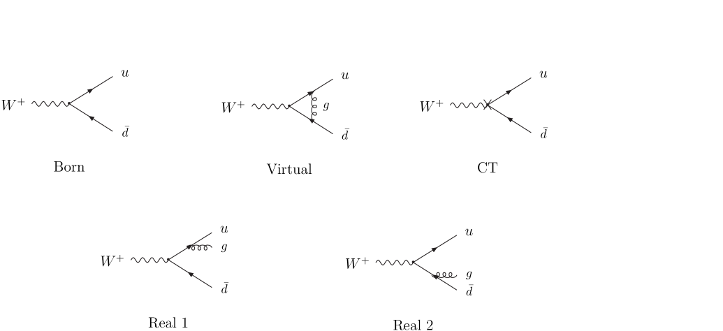
Figure 2: The Feynman diagrams in $W^{+}\rightarrow u\bar{d}$.

III.3 Corrections To $t\rightarrow bu\bar{d}$

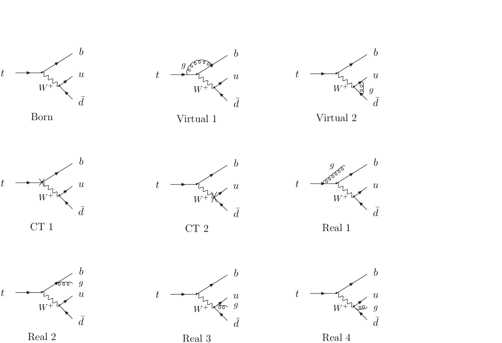
Figure 3: Feynman diagrams in $t\rightarrow bu\bar{d}$.

In this subsection, we present the analytical expressions of the top quark hadronic decay. The corresponding graphs are shown in Fig.3. As the mass of the top quark is 30 times larger than that of the bottom quark, we set the masses of all final states to be zero. The effect of the nonzero mass of the bottom quark is negligible in our results. Because of the intermediate-state $W$ boson in $t(p_{t})\rightarrow bW^{+}\rightarrow b(p_{b})u(p_{u})\bar{d}(p_{d})$, we treat this process in the complex mass schemeDenner:2005es ; Denner:2005fg . The Born amplitude squared with averaging over the initial-state spin and color is given by

$$|\overline{\mathcal{M}}_{0}|^{2}=\frac{3e^{4}}{2|s_{w}|^{4}}\frac{(1-y)y}{(1-y-z-r^{2})^{2}+(r^{2}w)^{2}},$$ (16)

where we have defined $(p_{t}-p_{d})^{2}=m_{t}^{2}y,(p_{t}-p_{u})^{2}=m_{t}^{2}z,r=\frac{m_{W}}{m_{t}},w=\frac{\Gamma_{W}}{m_{W}}$. Here, $y,z,r,w$ are all dimensionless variables. We keep the width of the W boson nonvanishing. The Born level decay width of this channel is

$$\Gamma_{0} = \frac{\alpha^{2}m_{t}}{64\pi|s_{w}|^{4}}\left[4r^{2}-2+2r^{2}\left(w^{2}r^{2}-3r^{2}+3\right)\ln(r^{2})\right.$$ (17)

$$+r^{2}\left(w^{2}r^{2}-3r^{2}+3\right)\ln(\frac{1+w^{2}}{\left(1-r^{2}\right)^{2}+\left(wr^{2}\right)^{2}})$$

$$\frac{6w^{2}r^{6}-2r^{6}-3w^{2}r^{4}+3r^{4}-1}{wr^{2}}$$

$$\left.\left(\tan^{-1}(w)+\tan^{-1}(\frac{wr^{2}}{1-r^{2}})-\pi\right)\right].$$

By expanding it in terms of $w$, to $\mathcal{O}{\left(w^{0}\right)}$ the above result can be expressed as

$$\Gamma_{0} = \frac{\alpha^{2}m_{t}}{64|s_{w}|^{4}r^{2}}\left[\left(1-r^{2}\right)\left(1+2r^{2}\right)w^{-1}+\right.$$ (18)

$$\left.\frac{\left(6r^{4}(1-r^{2})\ln(\frac{r^{2}}{1-r^{2}})+6r^{4}-3r^{2}-1\right)}{\pi}w^{0}+\mathcal{O}(w^{1})\right].$$

To leading order in $w$ the result is consistent with the narrow-width-approximation (NWA), $\Gamma_{t\rightarrow bu\bar{d}}=\Gamma_{t\rightarrow bW^{+}}\times\frac{\Gamma_{W^{+}\rightarrow u\bar{d}}}{\Gamma_{W}}$, with the Born width formulas of the top quark and W boson exhibited in two previous subsections. The second term is an off-shell correction, which is about $-0.6w$ relative to the first term with $r\approx 0.46$.

In naive or KKS $\gamma_{5}$ strategy within FDH regularization scheme, at QCD one loop level the squared matrix elements after renormalization with the initial-state averaged is given by

$$\left(|\overline{\mathcal{M}}_{v}|^{2}+|\overline{\mathcal{M}}_{ct}|^{2}\right)^{KKS}_{FDH} = |\overline{\mathcal{M}}_{0}|^{2}\frac{\alpha_{s}~{}C_{F}}{4\pi\Gamma(1-\epsilon)}\left(\frac{4\pi\mu^{2}}{m_{t}^{2}}\right)^{\epsilon}$$ (19)

$$\left[-\frac{6}{\epsilon^{2}}+\frac{4\ln((y+z)(1-y-z))-11}{\epsilon}+6\ln((y+z)(1-y-z))\right.$$

$$-2\ln^{2}(1-y-z)+4\ln(1-y-z)\ln(y+z)-4\ln^{2}(y+z)$$

$$\left.-\frac{2\ln(y+z)}{1-y}+4~{}\text{Li}_{2}(y+z)+\pi^{2}-25\right].$$

With the same rules as those stated in the previous subsections, the differences between other $\gamma_{5}$ strategies/regularization schemes and the FDH scheme in KKS $\gamma_{5}$ scheme are given by

$$\left(\delta|\overline{\mathcal{M}}_{v}|^{2}+\delta|\overline{\mathcal{M}}_{ct}|^{2}\right)^{KKS}_{HV/CDR} = |\overline{\mathcal{M}}_{0}|^{2}\frac{\alpha_{s}~{}C_{F}}{4\pi\Gamma(1-\epsilon)}\left(\frac{4\pi\mu^{2}}{m_{t}^{2}}\right)^{\epsilon}$$

$$\left[\frac{3(1-y-z)(y+z)}{y(1-y)}\frac{1}{\epsilon}-\frac{1}{2y(1-y)}\right.$$

$$\left(5y^{2}+22yz+11z^{2}-5y-11z\right.$$

$$\left.\left.+4(1-y-z)(y+z)\ln[(1-y-z)(y+z)]\right)\right],$$

$$\left(\delta|\overline{\mathcal{M}}_{v}|^{2}+\delta|\overline{\mathcal{M}}_{ct}|^{2}\right)^{BMHV}_{FDH} = |\overline{\mathcal{M}}_{0}|^{2}~{}\frac{\alpha_{s}~{}C_{F}}{\pi},$$

$$\left(\delta|\overline{\mathcal{M}}_{v}|^{2}+\delta|\overline{\mathcal{M}}_{ct}|^{2}\right)^{BMHV}_{HV/CDR} = |\overline{\mathcal{M}}_{0}|^{2}~{}\frac{5~{}\alpha_{s}~{}C_{F}}{4~{}\pi}.$$ (20)

To check our results, we also treat the numerators of loop amplitudes in four-dimensions by adding the $R_{2}$ terms at last. All of the results discussed above are recovered using this method. Because of the right-handed currentsShao:2011tg of the $R_{2}$ in the BMHV $\gamma_{5}$ scheme, the unrenormalized virtual contributions are the same within the same $\gamma_{5}$ treatment, and only the renormalization constants are different.

The remaining regularization scheme-dependent terms should be canceled by the real radiation part. The scheme-dependent terms in real corrections resulted from the soft and collinear region of phase space. The two cutoff phase space slicing method given by B.Harris and J.Owens is used hereHarris:2001sx . The analytical result within the FDH and KKS regularization scheme is given by

$$\left(|\overline{\mathcal{M}}_{sc}|^{2}\right)^{KKS}_{FDH} = |\overline{\mathcal{M}}_{0}|^{2}\frac{\alpha_{s}~{}C_{F}}{4\pi\Gamma(1-\epsilon)}\left(\frac{4\pi\mu^{2}}{m_{t}^{2}}\right)^{\epsilon}$$ (21)

$$\left[\frac{6}{\epsilon^{2}}-\frac{4\ln[(1-y-z)(y+z)]-11}{\epsilon}+2\ln^{2}[\frac{y~{}z}{1-y-z}]\right.$$

$$-2\ln^{2}(1-y)-2\ln^{2}(1-z)-2\ln^{2}(y+z)$$

$$+4\ln[(1-y)(1-z)(y+z)]\ln(\frac{\delta_{s}}{\delta_{c}})-9\ln(\delta_{c})$$

$$-4\ln(\delta_{s})-12\ln(\delta_{s})\ln(\delta_{c})+8\ln[(1-y-z)(y+z)]\ln(\delta_{s})$$

$$\left.+6\ln^{2}(\delta_{s})+4~{}\text{Li}_{2}[-\frac{1-y-z}{y~{}z}]+22-\frac{7\pi^{2}}{3}\right],$$

where $\delta_{s}$ and $\delta_{c}$ are two parameters to isolate the soft and collinear regions, respectively. The differences between other regularization schemes and the above scheme are

$$\left(\delta|\overline{\mathcal{M}}_{sc}|^{2}\right)^{KKS}_{HV/CDR} = -|\overline{\mathcal{M}}_{0}|^{2}\frac{\alpha_{s}~{}C_{F}}{4\pi\Gamma(1-\epsilon)}\left(\frac{4\pi\mu^{2}}{m_{t}^{2}}\right)^{\epsilon}$$

$$\left[\frac{3(1-y-z)(y+z)}{y(1-y)}\frac{1}{\epsilon}-\frac{1}{2y(1-y)}\right.$$

$$\left(5y^{2}+22yz+11z^{2}-5y-11z\right.$$

$$\left.\left.+4(1-y-z)(y+z)\ln[(1-y-z)(y+z)]\right)\right]$$

$$= -\left(\delta|\overline{\mathcal{M}}_{v}|^{2}+\delta|\overline{\mathcal{M}}_{ct}|^{2}\right)^{KKS}_{HV/CDR},$$

$$\left(\delta|\overline{\mathcal{M}}_{sc}|^{2}\right)^{BMHV}_{FDH} = 0,$$

$$\left(\delta|\overline{\mathcal{M}}_{sc}|^{2}\right)^{BMHV}_{HV/CDR} = |\overline{\mathcal{M}}_{0}|^{2}~{}\frac{3~{}\alpha_{s}~{}C_{F}}{4~{}\pi}.$$ (22)

In the BMHV $\gamma_{5}$ scheme, we also obtain the scheme-independent results after including the finite renormalization to the axial-vector currents. This was done in order to maintain the Ward identities as already shown in the last two subsections.

In the hard noncollinear phase space region, we treat the squared matrix element of $t(p_{t})\rightarrow b(p_{b})u(p_{u})d(p_{d})g(p_{g})$ in four dimensions. Dimensionless variables are redefined as follows:

$$(p_{t}-p_{g})^{2} = m_{t}^{2}~{}x,(p_{t}-p_{u})^{2}=m_{t}^{2}~{}y,(p_{t}-p_{d})^{2}=m_{t}^{2}~{}z,$$

$$(p_{u}+p_{d})^{2} = m_{t}^{2}~{}k,(p_{u}+p_{g})^{2}=m_{t}^{2}~{}l,r=\frac{m_{W}}{m_{t}},w=\frac{\Gamma_{W}}{m_{W}}.$$ (23)

The averaged squared amplitude is

$$|\overline{\mathcal{M}}_{real}|^{2} = \frac{3~{}e^{4}~{}g_{s}^{2}~{}C_{F}}{|s_{w}|^{4}~{}m_{t}^{2}}\left\{\frac{1}{(k-r^{2})^{2}+(wr^{2})^{2}}\frac{1}{(1-x)^{2}(1-y-z-k)}\right.$$ (24)

$$\left[\left(x-3\right)\left(k+l\right)^{2}k+2\left(xz-2x-y-4z+4\right)k^{2}\right.$$

$$+\left(\left(2xz-5x-4y-10z+11\right)l-x^{2}-y^{2}-7z^{2}+4y-4yz+15z\right.$$

$$\left.+\left(y^{2}-2y+z^{2}-7z+6\right)x-7\right)k+\left(1-z\right)\left(2-x-y-z\right)\left(1-x-2z\right)$$

$$\left.-\left(x+2y+2z-3\right)l^{2}-\left(x+2z-2\right)\left(x+2y+2z-3\right)l\right]$$

$$+\frac{1}{(2-x-y-z-r^{2})^{2}+(wr^{2})^{2}}\frac{1}{l(x+y+z+k+l-2)}$$

$$\left[\left(2-x-y-z\right)\left(1-z-k-l\right)^{2}-\left(k+l\right)\left(1-z-k-l\right)\right.$$

$$+\left.\left.\left(1-y\right)\left(l-y\left(2-x-y-z\right)\right)\right]\right\}$$

There are two kinds of Breit-Wigner distributions of the W boson in Eq.(24). The first term originated from the first two real diagrams, while the second is contributed by the last two final state radiative diagrams. Because of color flow, there is no interference observed between the first two and the last two diagrams.

IV Jet Algorithms And Phase Space

At high energy colliders, it was pointed out that the observed jets provided a view of parton (e.g. gluon and quark) interactions occurring at short distancesSterman:1977wj . At leading-order (LO) level, partons can be naively treated as jets, while at NLO level this coarse treatment often suffers from soft and collinear divergences. Therefore, an infrared-collinear safe jet definition is necessary in investigating strong interaction physics. Nowadays, these jet definitions play important roles in collider physics. Following the jet definition description in Refs.Catani:1993hr ; Catani:1992zp , the requirements implemented in a jet algorithms are as follows:

• simple to use in experiments and theoretical calculations,

• infrared and collinear safe,

• small hadronization corrections.

At hadron colliders, a well-defined jet algorithm must be able to factorize initial-state collinear singularities; they should also be isolated from the contamination of hadron remnants and underlying soft events.

Since the advent of jet production in electron-positron and hadron colliders, it has become one main tool in QCD research. Many kinds of algorithms have been proposed and developed. Essentially, the two classes of jet algorithms present mainly the clustering algorithmsBartel:1986ua ; Bethke:1988zc and the cone-type algorithmsSterman:1977wj ; Abe:1991ui ; Arnison:1983gw ; Salam:2007xv . In the present study, we focused on the three popular inclusive clustering algorithms, namely the $k_{\perp}$-clustering algorithmCatani:1993hr ; Catani:1992zp ; Ellis:1993tq ,the $\rm Cambridge/Aachen$ clustering algorithm(CA)Dokshitzer:1997in ; Wobisch:1998wt and the anti-$k_{\perp}$ clustering algorithmCacciari:2008gp respectively. These three inclusive clustering algorithms can be described uniformly:

• Define a distance $d_{ij}=min(p_{Ti}^{2r},p_{Tj}^{2r})\frac{\Delta R_{ij}}{R}$ between each pair of protojets i and j, as well as a distance $d_{iB}=p_{Ti}^{2r}$ between each protojet i and the beam,with $r=+1,0,-1$ corresponding to $k_{\perp}$,CA, and anti-$k_{\perp}$ respectively.

• Find the smallest of all the $d_{ij}$ and $d_{iB}$ and label it as $d_{min}$.

• If $d_{min}$ is a $d_{ij}$, then cluster protojets i and j as a new protojet with a selected combination procedure. If the distance between protojet i and the beam is the shortest, set the protojet i aside and leave it without any further clustering as a possible jet candidate.

• Repeat the items above until there is no protojet left.

• Perform some cuts (as in the experiment) to select jet(s) of interest.

Here $\Delta R_{ij}=\sqrt{\left(\eta_{i}-\eta_{j}\right)^{2}+\left(\phi_{i}-\phi_{j}\right)^{2}}$ ($\eta$ and $\phi$ are rapidity and azimuthal angle respectively). As $E$ can be measured at $e^{+}e^{-}$ colliders rather than only $p_{T}$ at hadronic colliders, one should use $E$ instead of $p_{T}$ and $\Delta S_{ij}=\sqrt{\Delta\theta_{ij}^{2}+\left(\sin{\frac{\theta_{i}+\theta_{j}}{2}}\Delta\phi_{ij}\right)^{2}}$ instead of $\Delta R_{ij}$ at $e^{+}e^{-}$ colliders.

It was also emphasized in Ref.Ellis:1993tq that traditional cone-type jet algorithms were related to clustering algorithms by the approximation $R_{cluster}=1.35\times R_{cone}$.

In the present study, we only used the three clustering algorithms with the E-scheme recombination to reconstruct our leading two jets from top quark hadronic decay in the next section (one can also use other recombination procedures as suggested in Ref.Catani:1993hr and references therein). In addition, we used hadron collider clustering algorithms and electron-positron collider clustering algorithms but without any cut in our calculation.

The last topic of this section is about a phase-space integration treatment. Given that we should reconstruct the four momenta of all final states in order to reconstruct two leading jets, we built up the n-particle phase space iteratively by nested integration over invariant masses and solid angles of outgoing particles, similar to the strategy in Ref.Hahn:2006qw .

V Results

The dijet invariant mass distributions with different clustering jet algorithms are presented in this section.

As discussed in the previous section, we used two variations of clustering jet algorithms in our top decay process in the c.m. frame of the top quark. In these two variations, we chose the distances defined at hadron colliders ( i.e. use $p_{T}$ ) and $e^{+}e^{-}$ colliders( i.e. use $E$), respectively, to reconstruct the final jets. Afterward, two leading jets in energy $E$ were chosen to construct their invariant mass $m_{jj}$. Here,we call the first types KT1, CA1, anti-KT1, while the second types are denoted as KT2, CA2, anti-KT2.

The following input parameters are used:

$$\alpha^{-1} = 129,\alpha_{s}(m_{Z})=0.119,$$

$$m_{W} = 80.399~{}GeV,\Gamma_{W}=2.085~{}GeV,m_{Z}=91.1876~{}GeV,\Gamma_{Z}=2.4952~{}GeV,$$

$$s_{w}^{2} = 1-\frac{m_{W}^{2}-i~{}m_{W}\Gamma_{W}}{m_{Z}^{2}-i~{}m_{Z}\Gamma_{Z}}=0.222657-1.11098\times 10^{-3}i,$$ (25)

with two groups of top quark mass and renormalization scale $\mu$ choices, i.e. $m_{t}=175~{}GeV$, $\mu=80.4~{}GeV$ and $m_{t}=172.5~{}GeV$, $\mu=m_{t}=172.5~{}GeV$.

We varied the parameter $R$ in the ${\rm CA1}$ jet algorithm and compared its influence on our results in Fig.4. Only when $R\geq 1.0$ in this algorithm, the infrared and collinear safety in each bin is maintained. Therefore, to ensure reliability, we choose $R=1.4$ in the first type jet algorithms and $R=1.3$ in the second ones for the rest of the paper. There are some interesting characters in these two figures. The variation of $R$ slightly changed our domain region (110-150 GeV) both in LO and NLO level. The larger $R$ reconstructs a smaller number of final jets; it makes the number of events in the last bin (170-175 GeV) larger with larger $R$. At LO, the distributions dropped sharply below 110 GeV and vanish below 100 GeV, as shown on the upper panel of Fig.4. In contrast, a NLO QCD correction resulted in the smooth descent of the low energy tail. The peak in Fig.4 (lower panel) between 80 GeV to 85 GeV is the W boson’s resonance.

Histograms in Figs.5 and 6 establish the influences of clustering jet algorithms to the dijet invariant mass distribution. The LO distributions reconstructed by various algorithms are almost indistinguishable. In comparison,there are some differences in the substructures of NLO histograms. The combination sequence of protojets is responsible for these tiny distinctions. Soft protojets may be clustered before the hard ones in $k_{\perp}$, while the situation may be totally different in anti-$k_{\perp}$. For comparison,we also plot the histograms with $m_{t}=172.5GeV$ and $\mu=172.5GeV$ in Fig.7.

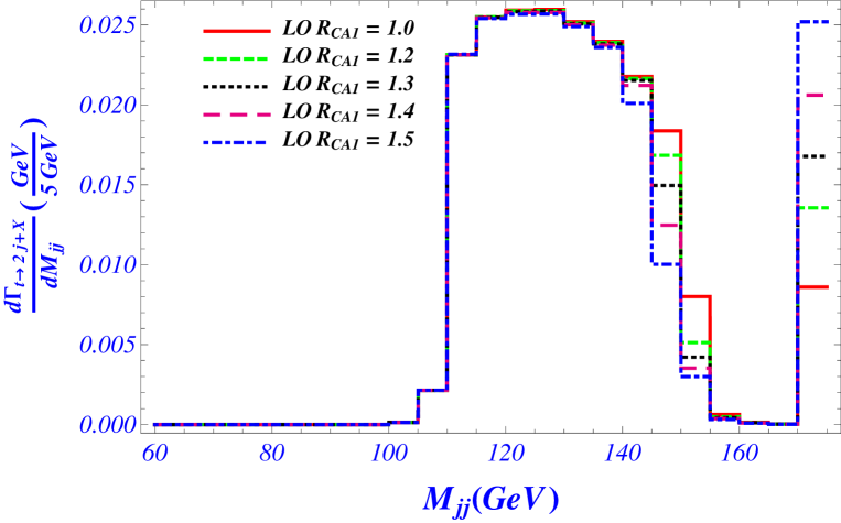
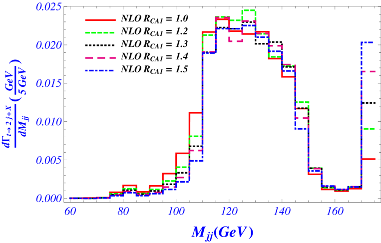
Figure 4: The LO (upper panel) and NLO (lower panel) dijet invariant mass distribution from top decay with different $R$ using the ${\rm CA1}$ clustering jet algorithm ($m_{t}=175~{}GeV,\mu=80.4~{}GeV$). Plotted are R=1.0 (solid line), 1.2 (short-dashed line), 1.3 (dotted line), 1.4 (long-dashed line), and 1.5 (dot-dashed line), respectively.

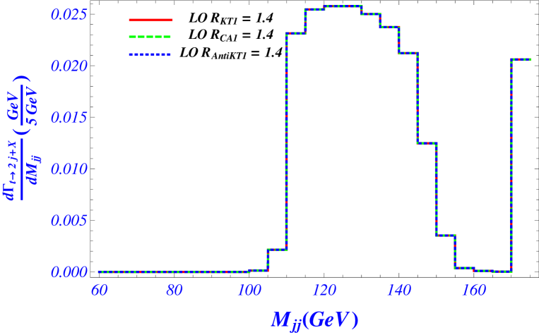
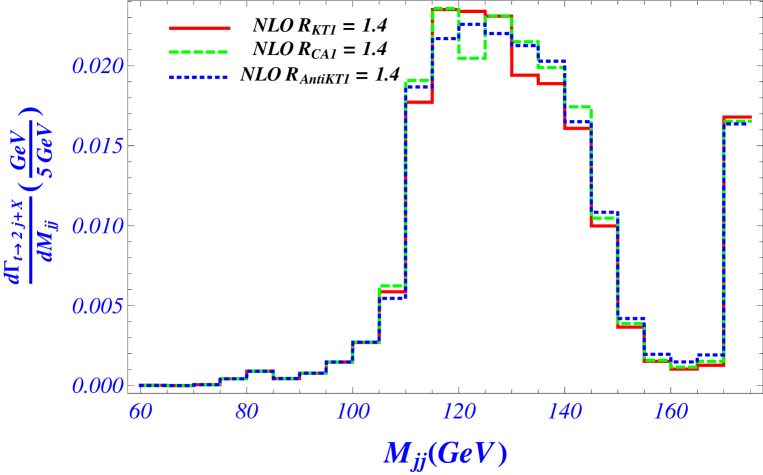
Figure 5: The influence on distribution with different clustering jet algorithms of the first type ($m_{t}=175~{}GeV,\mu=80.4~{}GeV$). LO is in the upper panel, while the lower panel is for the NLO results. Plots are KT1 (solid line), CA1 (dashed line), and anti-KT1 (dotted line).

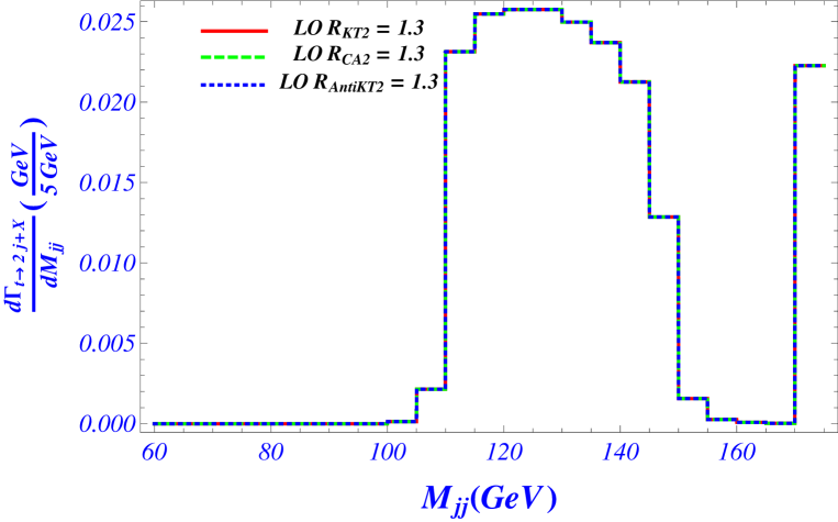
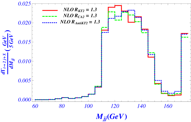
Figure 6: The influence on distribution with different clustering jet algorithms of the second type ($m_{t}=175~{}GeV,\mu=80.4~{}GeV$). LO is in the upper panel, while the lower panel is for the NLO results. Plots are KT2 (solid line), CA2 (dashed line), and anti-KT2 (dotted line).

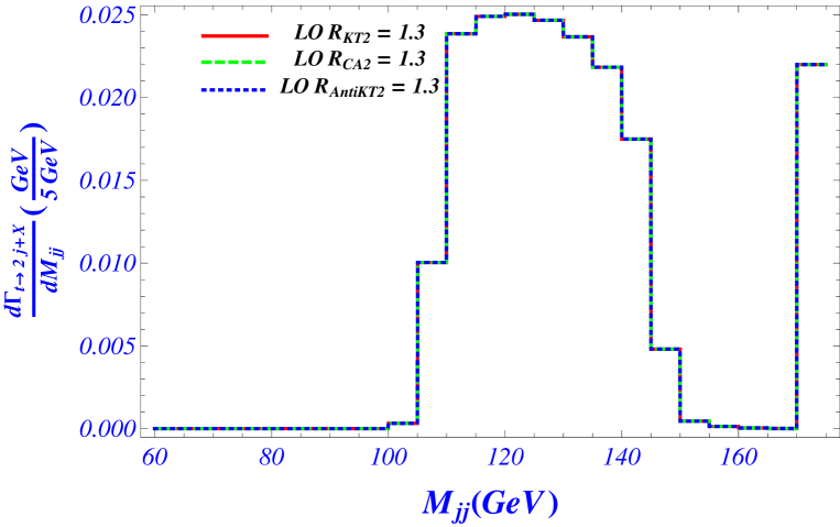
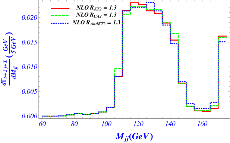
Figure 7: The influence on distribution with different clustering jet algorithms of the second type ($m_{t}=172.5~{}GeV,\mu=172.5~{}GeV$). LO is in the upper panel, while the lower panel is for the NLO results. Plots are similar to Fig.6.

VI Conclusions

We have performed QCD radiative corrections to the dijet production in the unpolarized top quark hadronic decay in the complex mass scheme. We carefully checked the independence of dimensional regularization schemes and $\gamma_{5}$ strategies in our analytical formalism. Applying different clustering jet definitions, we obtained our final dijet invariant mass distributions. The obtained dijet mass distributions from the top quark decay are useful to understand the top quark properties and also to distinguish these dijets from those produced via other sources. Therefore, these results are useful in investigating the recent CDF $Wjj$ anomaly and clarifying this interesting issue. Furthermore, a more careful investigation for top and W boson associated production at hadron colliders will be definitely needed.

- (1) CDF Collaboration, F. Abe et al., “Observation of top quark production in anti-p p collisions,” Phys. Rev. Lett. 74 (1995) 2626–2631, hep-ex/9503002.
- (2) D0 Collaboration, S. Abachi et al., “Observation of the top quark,” Phys. Rev. Lett. 74 (1995) 2632–2637, hep-ex/9503003.
- (3) B. W. Harris, E. Laenen, L. Phaf, Z. Sullivan, and S. Weinzierl, “The Fully differential single top quark cross-section in next to leading order QCD,” Phys. Rev. D66 (2002) 054024, hep-ph/0207055.
- (4) M. Jezabek and J. H. Kuhn, “QCD Corrections to Semileptonic Decays of Heavy Quarks,” Nucl. Phys. B314 (1989) 1.
- (5) J. M. Campbell, R. K. Ellis, and F. Tramontano, “Single top production and decay at next-to-leading order,” Phys. Rev. D70 (2004) 094012, hep-ph/0408158.
- (6) C. R. Schmidt, “Top quark production and decay at next-to-leading order in e+ e- annihilation,” Phys. Rev. D54 (1996) 3250–3265, hep-ph/9504434.
- (7) CDF Collaboration, T. Aaltonen et al., “Invariant Mass Distribution of Jet Pairs Produced in Association with a W boson in ppbar Collisions at sqrt(s) = 1.96 TeV,” Phys. Rev. Lett. 106 (2011) 171801, 1104.0699.
- (8) X.-G. He and B.-Q. Ma, “The CDF dijet excess from intrinsic quarks,” 1104.1894.
- (9) Z. Sullivan and A. Menon, “Standard model explanation of a CDF dijet excess in Wjj,”Phys. Rev. D83 (2011) 091504, 1104.3790.
- (10) T. Plehn and M. Takeuchi, “W+Jets at CDF: Evidence for Top Quarks,”J.Phys.G38 (2011) 095006, 1104.4087.
- (11) D0 Collaboration, V. M. Abazov et al., “Study of the dijet invariant mass distribution in final states at TeV,”Phys. Rev. Lett. 107 (2011) 011804, 1106.1921.
- (12) A. Denner and T. Sack, “The Top width,” Nucl. Phys. B358 (1991) 46–58.
- (13) A. Brandenburg, Z. G. Si, and P. Uwer, “QCD-corrected spin analysing power of jets in decays of polarized top quarks,” Phys. Lett. B539 (2002) 235–241, hep-ph/0205023.
- (14) J. Liu and Y.-P. Yao, “One loop radiative corrections to a heavy top decay in the standard model,” Int. J. Mod. Phys. A6 (1991) 4925–4948.
- (15) A. Czarnecki, “QCD corrections to the decay t W b in dimensional regularization,” Phys. Lett. B252 (1990) 467–470.
- (16) C. S. Li, R. J. Oakes, and T. C. Yuan, “QCD corrections to ,” Phys. Rev. D43 (1991) 3759–3762.
- (17) A. Ghinculov and Y.-P. Yao, “Exact O(g**2 alpha(s)) top decay width from general massive two-loop integrals,” Mod. Phys. Lett. A15 (2000) 925–930, hep-ph/0002211.
- (18) G. Eilam, R. R. Mendel, R. Migneron, and A. Soni, “Radiative corrections to top quark decay,” Phys. Rev. Lett. 66 (1991) 3105–3108.
- (19) A. Barroso, L. Brucher, and R. Santos, “Renormalization of the Cabibbo-Kobayashi-Maskawa matrix,” Phys. Rev. D62 (2000) 096003, hep-ph/0004136.
- (20) S. M. Oliveira, L. Brucher, R. Santos, and A. Barroso, “Electroweak corrections to the top quark decay,” Phys. Rev. D64 (2001) 017301, hep-ph/0011324.
- (21) A. Czarnecki and K. Melnikov, “Two-loop QCD corrections to top quark width,” Nucl. Phys. B544 (1999) 520–531, hep-ph/9806244.
- (22) K. G. Chetyrkin, R. Harlander, T. Seidensticker, and M. Steinhauser, “Second order QCD corrections to Gamma(),” Phys. Rev. D60 (1999) 114015, hep-ph/9906273.
- (23) M. Fischer, S. Groote, J. G. Korner, M. C. Mauser, and B. Lampe, “Polarized top decay into polarized W: at O(alpha(s)),” Phys. Lett. B451 (1999) 406–413, hep-ph/9811482.
- (24) M. Fischer, S. Groote, J. G. Korner, and M. C. Mauser, “Longitudinal, transverse plus and transverse minus W bosons in unpolarized top quark decays at O(alpha(s)),” Phys. Rev. D63 (2001) 031501, hep-ph/0011075.
- (25) M. Fischer, S. Groote, J. G. Korner, and M. C. Mauser, “Complete angular analysis of polarized top decay at O(alpha(s)),” Phys. Rev. D65 (2002) 054036, hep-ph/0101322.
- (26) A. A. Penin and A. A. Pivovarov, “Next-to-next-to-leading order relation between R() and Gamma(sl)() and precise determination of —V(cb)—,” Phys. Lett. B443 (1998) 264–268, hep-ph/9805344.
- (27) M. Jezabek and J. H. Kuhn, “The Top width: Theoretical update,” Phys. Rev. D48 (1993) R1910–R1913, hep-ph/9302295.
- (28) H. S. Do, S. Groote, J. G. Korner, and M. C. Mauser, “Electroweak and finite width corrections to top quark decays into transverse and longitudinal W bosons,” Phys. Rev. D67 (2003) 091501, hep-ph/0209185.
- (29) G. ’t Hooft and M. J. G. Veltman, “Regularization and Renormalization of Gauge Fields,” Nucl. Phys. B44 (1972) 189–213.
- (30) Z. Bern, A. De Freitas, L. J. Dixon, and H. L. Wong, “Supersymmetric regularization, two-loop QCD amplitudes and coupling shifts,” Phys. Rev. D66 (2002) 085002, hep-ph/0202271.
- (31) Z. Kunszt, A. Signer, and Z. Trocsanyi, “One loop helicity amplitudes for all 2 2 processes in QCD and N=1 supersymmetric Yang-Mills theory,” Nucl. Phys. B411 (1994) 397–442, hep-ph/9305239.
- (32) Z. Bern and D. A. Kosower, “The Computation of loop amplitudes in gauge theories,” Nucl. Phys. B379 (1992) 451–561.
- (33) Z. Bern, L. J. Dixon, D. C. Dunbar, and D. A. Kosower, “One-Loop n-Point Gauge Theory Amplitudes, Unitarity and Collinear Limits,” Nucl. Phys. B425 (1994) 217–260, hep-ph/9403226.
- (34) Z. Bern, L. J. Dixon, D. C. Dunbar, and D. A. Kosower, “Fusing gauge theory tree amplitudes into loop amplitudes,” Nucl. Phys. B435 (1995) 59–101, hep-ph/9409265.
- (35) W. Siegel, “Supersymmetric Dimensional Regularization via Dimensional Reduction,” Phys. Lett. B84 (1979) 193.
- (36) D. Kreimer, “THE gamma(5) PROBLEM AND ANOMALIES: A CLIFFORD ALGEBRA APPROACH,” Phys. Lett. B237 (1990) 59.
- (37) P. Breitenlohner and D. Maison, “Dimensional Renormalization and the Action Principle,” Commun. Math. Phys. 52 (1977) 11–38.
- (38) P. Breitenlohner and D. Maison, “Dimensionally Renormalized Green’s Functions for Theories with Massless Particles. 1,” Commun. Math. Phys. 52 (1977) 39.
- (39) P. Breitenlohner and D. Maison, “Dimensionally Renormalized Green’s Functions for Theories with Massless Particles. 2,” Commun. Math. Phys. 52 (1977) 55.
- (40) D. Kreimer, “The Role of gamma(5) in dimensional regularization,” hep-ph/9401354.
- (41) J. G. Korner, D. Kreimer, and K. Schilcher, “A Practicable gamma(5) scheme in dimensional regularization,” Z. Phys. C54 (1992) 503–512.
- (42) J. G. Korner, N. Nasrallah, and K. Schilcher, “EVALUATION OF THE FLAVOR CHANGING VERTEX b s H USING THE BREITENLOHNER-MAISON-’t HOOFT-VELTMAN gamma(5) SCHEME,” Phys. Rev. D41 (1990) 888.
- (43) A. J. Buras, “Weak Hamiltonian, CP violation and rare decays,” hep-ph/9806471.
- (44) C. P. Martin and D. Sanchez-Ruiz, “Action principles, restoration of BRS symmetry and the renormalization group equation for chiral nonAbelian gauge theories in dimensional renormalization with a nonanticommuting gamma(5),” Nucl. Phys. B572 (2000) 387, hep-th/9905076.
- (45) C. Schubert, “THE YUKAWA MODEL AS AN EXAMPLE FOR DIMENSIONAL RENORMALIZATION WITH gamma(5),” Nucl. Phys. B323 (1989) 478.
- (46) M. Pernici, M. Raciti and F. Riva, “Dimensional renormalization of Yukawa theories via Wilsonian methods,” Nucl. Phys. B577 (2000) 293, hep-th/9912248.
- (47) M. Pernici, “Seminaive dimensional renormalization,” Nucl. Phys. B582 (2000) 733, hep-th/9912278.
- (48) R. Ferrari, A. Le Yaouanc, L. Oliver and J. C. Raynal, “Gauge invariance and dimensional regularization with gamma(5) in flavor changing neutral processes,” Phys. Rev. D52 (1995) 3036.
- (49) M. Pernici and M. Raciti, “Axial current in QED and seminaive dimensional renormalization,” Phys. Lett. B513 (2001) 421, hep-th/0003062.
- (50) G. Altarelli and G. Parisi, “Asymptotic Freedom in Parton Language,” Nucl. Phys. B126 (1977) 298.
- (51) S. Catani, M. H. Seymour, and Z. Trocsanyi, “Regularization scheme independence and unitarity in QCD cross sections,” Phys. Rev. D55 (1997) 6819–6829, hep-ph/9610553.
- (52) W. T. Giele and E. W. N. Glover, “Higher order corrections to jet cross-sections in e+ e- annihilation,” Phys. Rev. D46, 1980 (1992).
- (53) W. T. Giele, E. W. N. Glover and D. A. Kosower, “Higher order corrections to jet cross-sections in hadron colliders,” Nucl. Phys. B403, 633 (1993), hep-ph/9302225.
- (54) T. Hahn, “Generating Feynman diagrams and amplitudes with FeynArts 3,” Comput. Phys. Commun. 140 (2001) 418–431, hep-ph/0012260.
- (55) G. Altarelli, R. K. Ellis, and G. Martinelli, “Large Perturbative Corrections to the Drell-Yan Process in QCD,” Nucl. Phys. B157 (1979) 461.
- (56) A. Denner and T. Sack, “The W boson width,” Z. Phys. C46 (1990) 653–663.
- (57) A. Denner, S. Dittmaier, M. Roth and L. H. Wieders, “Complete electroweak O(alpha) corrections to charged-current 4 fermion processes,” Phys. Lett. B612, 223 (2005), hep-ph/0502063.
- (58) A. Denner, S. Dittmaier, M. Roth and L. H. Wieders, “Electroweak corrections to charged-current 4 fermion processes: Technical details and further results,” Nucl. Phys. B724, 247 (2005), hep-ph/0505042.
- (59) R. K. Ellis and G. Zanderighi, “Scalar one-loop integrals for QCD,” JHEP 0802, 002 (2008), 0712.1851.
- (60) H. S. Shao, Y. J. Zhang and K. T. Chao, “Feynman Rules for the Rational Part of the Standard Model One-loop Amplitudes in the ’t Hooft-Veltman Scheme,”JHEP 09 (2011) 048, 1106.5030.
- (61) B. W. Harris and J. F. Owens, “The two cutoff phase space slicing,” Phys. Rev. D65 (2002) 094032, hep-ph/0102128.
- (62) G. F. Sterman and S. Weinberg, “Jets from Quantum Chromodynamics,” Phys. Rev. Lett. 39 (1977) 1436.
- (63) S. Catani, Y. L. Dokshitzer, M. H. Seymour, and B. R. Webber, “Longitudinally invariant K(t) clustering algorithms for hadron hadron collisions,” Nucl. Phys. B406 (1993) 187–224.
- (64) S. Catani, Y. L. Dokshitzer, and B. R. Webber, “The K-perpendicular clustering algorithm for jets in deep inelastic scattering and hadron collisions,” Phys. Lett. B285 (1992) 291–299.
- (65) JADE Collaboration, W. Bartel et al., “Experimental Studies on Multi-Jet Production in e+ e- Annihilation at PETRA Energies,” Z. Phys. C33 (1986) 23.
- (66) JADE Collaboration, S. Bethke et al., “Experimental Investigation of the Energy Dependence of the Strong Coupling Strength,” Phys. Lett. B213 (1988) 235.
- (67) CDF Collaboration, F. Abe et al., “The Topology of three jet events in anti-p p collisions at S**(1/2) = 1.8-TeV,” Phys. Rev. D45 (1992) 1448–1458.
- (68) UA1 Collaboration, G. Arnison et al., “Hadronic Jet Production at the CERN Proton - anti-Proton Collider,” Phys. Lett. B132 (1983) 214.
- (69) G. P. Salam and G. Soyez, “A practical Seedless Infrared-Safe Cone jet algorithm,” JHEP 05 (2007) 086, 0704.0292.
- (70) S. D. Ellis and D. E. Soper, “Successive combination jet algorithm for hadron collisions,” Phys. Rev. D48 (1993) 3160–3166, hep-ph/9305266.
- (71) Y. L. Dokshitzer, G. D. Leder, S. Moretti, and B. R. Webber, “Better Jet Clustering Algorithms,” JHEP 08 (1997) 001, hep-ph/9707323.
- (72) M. Wobisch and T. Wengler, “Hadronization corrections to jet cross sections in deep- inelastic scattering,” hep-ph/9907280.
- (73) M. Cacciari, G. P. Salam, and G. Soyez, “The anti- jet clustering algorithm,” JHEP 04 (2008) 063, 0802.1189.
- (74) T. Hahn and M. Rauch, “News from FormCalc and LoopTools,” Nucl. Phys. Proc. Suppl. 157 (2006) 236–240, hep-ph/0601248.