¹¹institutetext: Tata Institute of Fundamental Research, Homi Bhabha Road, Mumbai 400005, India ¹¹email: bhaswati@tifr.res.in ²²institutetext: Instituto Radioastronomía Milimétrica, Av. Divina Pastora 7, Nucleo Central, E-18012 Granada, Spain ³³institutetext: University of Massachusetts, Department of Astronomy, LGRT-B 619E, Amherst, MA 01003, USA ⁴⁴institutetext: Universidad de Granada, E-18012 Granada, Spain ⁵⁵institutetext: Department of Radio and Space Science, Onsala Observatory, Chalmers University of Technology, S-43992 Onsala, Sweden ⁶⁶institutetext: Laboratoire d’Astrophysique de Bordeaux, Université Bordeaux 1, Observatoire de Bordeaux, OASU, UMR 5804, CNRS/INSU, B.P. 89, Floirac F-33270 ⁷⁷institutetext: Observatoire de Paris, LERMA, CNRS, 61 Av. de lâ ? ?Observatoire, 75014 Paris, France ⁸⁸institutetext: Observatorio Astronómico Nacional (OAN) - Observatorio de Madrid, Alfonso XII 3, 28014 Madrid, Spain ⁹⁹institutetext: Max Planck Institut für Radioastronomie, Auf dem Hügel 69, D- 53121 Bonn, Germany ¹⁰¹⁰institutetext: Leiden Observatory, Leiden University, PO Box 9513, NL 2300 RA Leiden, The Netherlands ¹¹¹¹institutetext: IPAC, MS 100-22 California Institute of Technology, Pasadena, CA 91125, USA ¹²¹²institutetext: Department of Astronomy, Cornell University, Ithaca, NY 14853 ¹³¹³institutetext: KOSMA, I. Physikalisches Institut, Universität zu Köln, Zülpicher Strasse 77, D-50937 Köln, Germany ¹⁴¹⁴institutetext: Institute of Astronomy, University of Cambridge, Madingley Road, Cambridge CB3 0HA, England ¹⁵¹⁵institutetext: SRON Netherlands Institute for Space Research, Landleven 12, 9747 AD Groningen, The Netherlands 19 ¹⁶¹⁶institutetext: SUPA, Institute for Astronomy, University of Edinburgh, Royal Observatory, Blackford Hill, Edinburgh EH9 3HJ, UK 7

The Herschel M33 extended survey (HerM33es): PACS spectroscopy of the star forming region BCLMP 302 ^†^†thanks: Herschel is an ESA space observatory with science instruments provided by European-led Principal Investigator consortia and with important participation from NASA.

B. Mookerjea The Herschel M33 extended survey (HerM33es): PACS spectroscopy of the star forming region BCLMP 302 ^†^†thanks: Herschel is an ESA space observatory with science instruments provided by European-led Principal Investigator consortia and with important participation from NASA.The Herschel M33 extended survey (HerM33es): PACS spectroscopy of the star forming region BCLMP 302 ^†^†thanks: Herschel is an ESA space observatory with science instruments provided by European-led Principal Investigator consortia and with important participation from NASA. C. Kramer The Herschel M33 extended survey (HerM33es): PACS spectroscopy of the star forming region BCLMP 302 ^†^†thanks: Herschel is an ESA space observatory with science instruments provided by European-led Principal Investigator consortia and with important participation from NASA.The Herschel M33 extended survey (HerM33es): PACS spectroscopy of the star forming region BCLMP 302 ^†^†thanks: Herschel is an ESA space observatory with science instruments provided by European-led Principal Investigator consortia and with important participation from NASA. C. Buchbender The Herschel M33 extended survey (HerM33es): PACS spectroscopy of the star forming region BCLMP 302 ^†^†thanks: Herschel is an ESA space observatory with science instruments provided by European-led Principal Investigator consortia and with important participation from NASA.The Herschel M33 extended survey (HerM33es): PACS spectroscopy of the star forming region BCLMP 302 ^†^†thanks: Herschel is an ESA space observatory with science instruments provided by European-led Principal Investigator consortia and with important participation from NASA. M. Boquien The Herschel M33 extended survey (HerM33es): PACS spectroscopy of the star forming region BCLMP 302 ^†^†thanks: Herschel is an ESA space observatory with science instruments provided by European-led Principal Investigator consortia and with important participation from NASA.The Herschel M33 extended survey (HerM33es): PACS spectroscopy of the star forming region BCLMP 302 ^†^†thanks: Herschel is an ESA space observatory with science instruments provided by European-led Principal Investigator consortia and with important participation from NASA. S. Verley The Herschel M33 extended survey (HerM33es): PACS spectroscopy of the star forming region BCLMP 302 ^†^†thanks: Herschel is an ESA space observatory with science instruments provided by European-led Principal Investigator consortia and with important participation from NASA.The Herschel M33 extended survey (HerM33es): PACS spectroscopy of the star forming region BCLMP 302 ^†^†thanks: Herschel is an ESA space observatory with science instruments provided by European-led Principal Investigator consortia and with important participation from NASA. M. Relaño The Herschel M33 extended survey (HerM33es): PACS spectroscopy of the star forming region BCLMP 302 ^†^†thanks: Herschel is an ESA space observatory with science instruments provided by European-led Principal Investigator consortia and with important participation from NASA.The Herschel M33 extended survey (HerM33es): PACS spectroscopy of the star forming region BCLMP 302 ^†^†thanks: Herschel is an ESA space observatory with science instruments provided by European-led Principal Investigator consortia and with important participation from NASA. G. Quintana-Lacaci The Herschel M33 extended survey (HerM33es): PACS spectroscopy of the star forming region BCLMP 302 ^†^†thanks: Herschel is an ESA space observatory with science instruments provided by European-led Principal Investigator consortia and with important participation from NASA.The Herschel M33 extended survey (HerM33es): PACS spectroscopy of the star forming region BCLMP 302 ^†^†thanks: Herschel is an ESA space observatory with science instruments provided by European-led Principal Investigator consortia and with important participation from NASA. S. Aalto The Herschel M33 extended survey (HerM33es): PACS spectroscopy of the star forming region BCLMP 302 ^†^†thanks: Herschel is an ESA space observatory with science instruments provided by European-led Principal Investigator consortia and with important participation from NASA.The Herschel M33 extended survey (HerM33es): PACS spectroscopy of the star forming region BCLMP 302 ^†^†thanks: Herschel is an ESA space observatory with science instruments provided by European-led Principal Investigator consortia and with important participation from NASA. J. Braine The Herschel M33 extended survey (HerM33es): PACS spectroscopy of the star forming region BCLMP 302 ^†^†thanks: Herschel is an ESA space observatory with science instruments provided by European-led Principal Investigator consortia and with important participation from NASA.The Herschel M33 extended survey (HerM33es): PACS spectroscopy of the star forming region BCLMP 302 ^†^†thanks: Herschel is an ESA space observatory with science instruments provided by European-led Principal Investigator consortia and with important participation from NASA. D. Calzetti The Herschel M33 extended survey (HerM33es): PACS spectroscopy of the star forming region BCLMP 302 ^†^†thanks: Herschel is an ESA space observatory with science instruments provided by European-led Principal Investigator consortia and with important participation from NASA.The Herschel M33 extended survey (HerM33es): PACS spectroscopy of the star forming region BCLMP 302 ^†^†thanks: Herschel is an ESA space observatory with science instruments provided by European-led Principal Investigator consortia and with important participation from NASA. F. Combes The Herschel M33 extended survey (HerM33es): PACS spectroscopy of the star forming region BCLMP 302 ^†^†thanks: Herschel is an ESA space observatory with science instruments provided by European-led Principal Investigator consortia and with important participation from NASA.The Herschel M33 extended survey (HerM33es): PACS spectroscopy of the star forming region BCLMP 302 ^†^†thanks: Herschel is an ESA space observatory with science instruments provided by European-led Principal Investigator consortia and with important participation from NASA. S. Garcia-Burillo The Herschel M33 extended survey (HerM33es): PACS spectroscopy of the star forming region BCLMP 302 ^†^†thanks: Herschel is an ESA space observatory with science instruments provided by European-led Principal Investigator consortia and with important participation from NASA.The Herschel M33 extended survey (HerM33es): PACS spectroscopy of the star forming region BCLMP 302 ^†^†thanks: Herschel is an ESA space observatory with science instruments provided by European-led Principal Investigator consortia and with important participation from NASA. P. Gratier The Herschel M33 extended survey (HerM33es): PACS spectroscopy of the star forming region BCLMP 302 ^†^†thanks: Herschel is an ESA space observatory with science instruments provided by European-led Principal Investigator consortia and with important participation from NASA.The Herschel M33 extended survey (HerM33es): PACS spectroscopy of the star forming region BCLMP 302 ^†^†thanks: Herschel is an ESA space observatory with science instruments provided by European-led Principal Investigator consortia and with important participation from NASA. C. Henkel The Herschel M33 extended survey (HerM33es): PACS spectroscopy of the star forming region BCLMP 302 ^†^†thanks: Herschel is an ESA space observatory with science instruments provided by European-led Principal Investigator consortia and with important participation from NASA.The Herschel M33 extended survey (HerM33es): PACS spectroscopy of the star forming region BCLMP 302 ^†^†thanks: Herschel is an ESA space observatory with science instruments provided by European-led Principal Investigator consortia and with important participation from NASA. F. Israel The Herschel M33 extended survey (HerM33es): PACS spectroscopy of the star forming region BCLMP 302 ^†^†thanks: Herschel is an ESA space observatory with science instruments provided by European-led Principal Investigator consortia and with important participation from NASA.The Herschel M33 extended survey (HerM33es): PACS spectroscopy of the star forming region BCLMP 302 ^†^†thanks: Herschel is an ESA space observatory with science instruments provided by European-led Principal Investigator consortia and with important participation from NASA. S. Lord The Herschel M33 extended survey (HerM33es): PACS spectroscopy of the star forming region BCLMP 302 ^†^†thanks: Herschel is an ESA space observatory with science instruments provided by European-led Principal Investigator consortia and with important participation from NASA.The Herschel M33 extended survey (HerM33es): PACS spectroscopy of the star forming region BCLMP 302 ^†^†thanks: Herschel is an ESA space observatory with science instruments provided by European-led Principal Investigator consortia and with important participation from NASA. T. Nikola The Herschel M33 extended survey (HerM33es): PACS spectroscopy of the star forming region BCLMP 302 ^†^†thanks: Herschel is an ESA space observatory with science instruments provided by European-led Principal Investigator consortia and with important participation from NASA.The Herschel M33 extended survey (HerM33es): PACS spectroscopy of the star forming region BCLMP 302 ^†^†thanks: Herschel is an ESA space observatory with science instruments provided by European-led Principal Investigator consortia and with important participation from NASA. M. Röllig The Herschel M33 extended survey (HerM33es): PACS spectroscopy of the star forming region BCLMP 302 ^†^†thanks: Herschel is an ESA space observatory with science instruments provided by European-led Principal Investigator consortia and with important participation from NASA.The Herschel M33 extended survey (HerM33es): PACS spectroscopy of the star forming region BCLMP 302 ^†^†thanks: Herschel is an ESA space observatory with science instruments provided by European-led Principal Investigator consortia and with important participation from NASA. G. Stacey The Herschel M33 extended survey (HerM33es): PACS spectroscopy of the star forming region BCLMP 302 ^†^†thanks: Herschel is an ESA space observatory with science instruments provided by European-led Principal Investigator consortia and with important participation from NASA.The Herschel M33 extended survey (HerM33es): PACS spectroscopy of the star forming region BCLMP 302 ^†^†thanks: Herschel is an ESA space observatory with science instruments provided by European-led Principal Investigator consortia and with important participation from NASA. F. S. Tabatabaei The Herschel M33 extended survey (HerM33es): PACS spectroscopy of the star forming region BCLMP 302 ^†^†thanks: Herschel is an ESA space observatory with science instruments provided by European-led Principal Investigator consortia and with important participation from NASA.The Herschel M33 extended survey (HerM33es): PACS spectroscopy of the star forming region BCLMP 302 ^†^†thanks: Herschel is an ESA space observatory with science instruments provided by European-led Principal Investigator consortia and with important participation from NASA. F. van der Tak The Herschel M33 extended survey (HerM33es): PACS spectroscopy of the star forming region BCLMP 302 ^†^†thanks: Herschel is an ESA space observatory with science instruments provided by European-led Principal Investigator consortia and with important participation from NASA.The Herschel M33 extended survey (HerM33es): PACS spectroscopy of the star forming region BCLMP 302 ^†^†thanks: Herschel is an ESA space observatory with science instruments provided by European-led Principal Investigator consortia and with important participation from NASA. P. van der Werf The Herschel M33 extended survey (HerM33es): PACS spectroscopy of the star forming region BCLMP 302 ^†^†thanks: Herschel is an ESA space observatory with science instruments provided by European-led Principal Investigator consortia and with important participation from NASA.The Herschel M33 extended survey (HerM33es): PACS spectroscopy of the star forming region BCLMP 302 ^†^†thanks: Herschel is an ESA space observatory with science instruments provided by European-led Principal Investigator consortia and with important participation from NASA.The Herschel M33 extended survey (HerM33es): PACS spectroscopy of the star forming region BCLMP 302 ^†^†thanks: Herschel is an ESA space observatory with science instruments provided by European-led Principal Investigator consortia and with important participation from NASA.The Herschel M33 extended survey (HerM33es): PACS spectroscopy of the star forming region BCLMP 302 ^†^†thanks: Herschel is an ESA space observatory with science instruments provided by European-led Principal Investigator consortia and with important participation from NASA.

(Received …; accepted …)

Abstract

Context. The emission line of [C ii] at $158\,\mu$ m is one of the strongest cooling lines of the interstellar medium (ISM) in galaxies.

Aims. Disentangling the relative contributions of the different ISM phases to [C ii] emission, is a major topic of the HerM33es program, a Herschel key project to study the ISM in the nearby spiral galaxy M33.

Methods. Using PACS, we have mapped the emission of [C ii] 158 $\,\mu$ m, [O i] 63 $\,\mu$ m, and other FIR lines in a 2′ $\times$ 2′ region of the northern spiral arm of M33, centered on the H ii region BCLMP 302. At the peak of H $\alpha$ emission, we have observed in addition a velocity resolved [C ii] spectrum using HIFI. We use scatterplots to compare these data with PACS 160 $\,\mu$ m continuum maps, and with maps of CO and H i data, at a common resolution of 12″ or 50 pc. Maps of H $\alpha$ and 24 $\,\mu$ m emission observed with Spitzer are used to estimate the SFR. We have created maps of the [C ii] and [O i] 63 $\,\mu$ m emission and detected [N ii] 122 $\,\mu$ m and [N iii] 57 $\,\mu$ m at individual positions.

Results. The [C ii] line observed with HIFI is significantly broader than that of CO, and slightly blue-shifted. In addition, there is little spatial correlation between [C ii] observed with PACS and CO over the mapped region. There is even less spatial correlation between [C ii] and the atomic gas traced by H i. Detailed comparison of the observed intensities towards the H ii region with models of photo ionization and photon dominated regions, confirms that a significant fraction, 20–30%, of the observed [C ii] emission stems from the ionized gas and not from the molecular cloud. The gas heating efficiency, using the ratio between [C ii] and the TIR as a proxy, varies between 0.07 and 1.5%, with the largest variations found outside the H ii region.

Key Words.:

ISM: clouds - ISM: HII regions - ISM: photon-dominated regions (PDR) - Galaxies: individual: M33 - Galaxies: ISM - Galaxies: star formation

1 Introduction

Refer to caption — Figure 1: 250 $\mu$ m Herschel-SPIRE dust continuum image of the northern spiral arm of M33 along with the locations of the prominent H ii regions NGC 604, NGC 595, IC 142, BCLMP 302, and BCLMP 691. The rectangle delineates the area observed with PACS and HIFI, which is centered on BCLMP 302. The white circles indicate the positions and $70^{\prime\prime}$ beam of ISO/LWS observations done within the BCLMP 302 region. The white ellipse delineates 2 kpc galacto centric distance. The two parallel lines running along the major axis of M33, mark the strip for which we plan to observe the [C ii] and other FIR lines using PACS and HIFI.

The thermal balance and dynamics of the interstellar medium in galaxies, is best studied through spectroscopic observations of its major cooling lines: [C i], [C ii], and [O i] trace the transition regions between the atomic and molecular gas, while CO traces the dense molecular gas that provides the reservoir for stars to form. Most of the important cooling lines lie in the far-infrared and submillimeter regime. Therefore, it is difficult or impossible to study them with ground-based telescopes, while previous space-based telescopes provided low sensitivity and coarse angular resolution. The infrared line emission is mostly optically thin and can be traced throughout the densest regions in galaxies, allowing an unhindered view of the ISM. Herschel provides, for the first time, an opportunity to image the major tracers of the ISM at a sensitivity, spectral and spatial resolution that allows to study the interplay between star formation and the active ISM throughout our Milky Way and in nearby galaxies.

The two fine structure lines of [C ii] at 158 $\,\mu$ m and [O i] at 63 $\mu$ m, are the strongest cooling lines of the ISM, carrying up to a few percent of the total energy emitted from galaxies in the far-infrared wavelengths. The [C ii] line lies 92 K above the ground state with a critical density for collisions with H of $3\times 10^{3}$ cm^-3 (Kaufman et al. 1999). While both lines are thought to trace photon-dominated regions (PDRs) at the FUV irradiated surfaces of molecular clouds, it has been realized early-on that a non-negligible fraction of the [C ii] emission may stem from the ionized medium (Heiles 1994). Owing to its higher upper energy level (228 K) and higher critical density of $\simeq 5\times 10^{5}$ cm^-3, the [O i] 63 $\,\mu$ m line is a more dominant coolant in warmer and denser neutral regions (e.g. Röllig et al. 2006).

The [C ii] line together with the [O i] line are diagnostics to infer the physical conditions in the gas, its temperatures, densities, and radiation fields, by comparing the intensities and their ratios with predictions of PDR models (e.g., Tielens & Hollenbach 1985; Wolfire et al. 1990; Kaufman et al. 1999; Röllig et al. 2007; Ferland et al. 1998). Previous observational studies of [C ii] emission from external galaxies include the statistical studies by Crawford et al. (1985); Stacey et al. (1991); Malhotra et al. (2001). More recently the [C ii] emission from a few individual galaxies e.g., LMC (Israel et al. 1996), M51 (Nikola et al. 2001; Kramer et al. 2005), NGC 6946 (Madden et al. 1993; Contursi et al. 2002), M83 (Kramer et al. 2005), NGC 1313 (Contursi et al. 2002), M 31 (Rodriguez-Fernandez et al. 2006), NGC1097 (Contursi et al. 2002; Beirão et al. 2010) have been observed. These papers explore the origin of the [C ii] emission. Of these studies, the study of LMC by Israel et al. (1996) was at a resolution of 16 pc and Rodriguez-Fernandez et al. (2006) resolved the spiral arms of M 31 at spatial scales of 300 pc.

In addition to [C ii] and [O i] 63 $\mu$ m, there are several additional FIR lines, the mid- $J$ CO transitions, and lines of single and double ionized N and O which provide information about the gas density (multiple transitions of the same ions), hardness of the stellar radiation field (ratio of intensities of two ionization states of the same species), and ionizing flux. In particular the [N ii] lines at 122 and 205 $\,\mu$ m allow us to estimate the density of the ionized gas, which is a key parameter to model the [C ii] emission stemming from the ionized gas.

Although much detailed information can be obtained by studying nearby (Milky Way) sites of star formation, a more comprehensive view is possible with a nearby moderately inclined galaxy such as M33. M 33 is a nearby, moderately metal poor late-type spiral galaxy with no bulge or ring, classified as SA(s)cd. It is the 3rd largest member of the Local Group. Its mass, size, and average metallicity are similar to those of the Large Magellanic Cloud (LMC). M33 hosts some of the brightest H ii complexes in the Local Group. NGC 604 is the second brightest H ii region after 30 Doradus in the LMC. Its inclination ( $i=56^{\circ}$ ) (Regan & Vogel 1994) yields a small line-of-sight depth which allows to study individual cloud complexes not suffering from distance ambiguities and confusion like Galactic observations do. Its close distance of 840 kpc (Freedman et al. 1991) provides a spatial resolution of 50 pc at $12^{\prime\prime}$ , allowing us to resolve giant molecular associations in its disk with current single dish millimeter and far-infrared telescopes like the IRAM 30m telescope and Herschel. Its recent star formation activity, together with the absence of signs of recent mergers, makes M 33 an ideal source to study the interplay of gas, dust, and star formation in its disk. This is the aim of the open time key program “Herschel M33 extended survey” HerM33es (Kramer et al. 2010). To this end we are surveying the major cooling lines, notably [C ii], [O i], [N ii], as well as the dust spectral energy distribution (SED) using all three instruments on board of Herschel, HIFI, PACS, and SPIRE. We also use ancillary observations of H $\alpha$ , H i, CO and dust continuum at 24 $\,\mu$ m. The HerM33es PACS and HIFI spectral line observations will focus on a number of individual regions along the major axis of M 33 which will initially be presented individually.

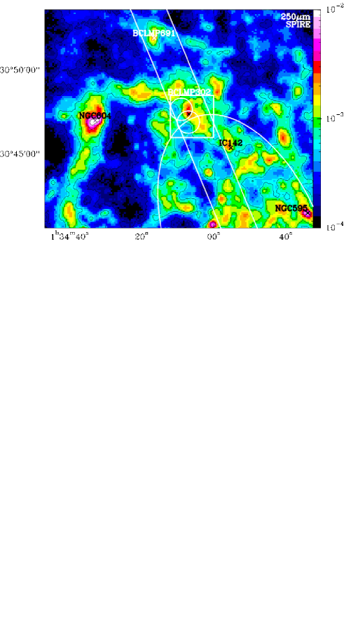
Here, we present first spectroscopic results obtained for BCLMP302, one of the brightest H ii regions of M33. We discuss a $2^{\prime}\times 2^{\prime}$ ( $\sim$ 0.5 kpc $\times$ 0.5 kpc) field in the northern spiral arm at a galactocentric distance of 2 kpc (Figure 1). This region lies along the major axis of M33, and houses one of the bright H ii regions, BCLMP 302 (Boulesteix et al. 1974; Israel & van der Kruit 1974). Using ISO/SWS, Willner & Nelson-Patel (2002) studied Neon abundances of H ii regions in M33, including BCLMP 302. Rubin et al. (2008) used Spitzer-IRS to map the emission lines of [S iv] 10.51, H(7–6) 12.37, [Ne ii] 12.8, [Ne iii] 15.56 and [S iii] 18.71 $\,\mu$ m in 25 H ii regions in M33, including BCLMP 302. ISO/LWS [C ii] unresolved spectra at $\sim 70^{\prime\prime}$ resolution (Gry et al. 2003) are available for this region from the archive. Here, we present PACS maps of [C ii] and [O i] 63 $\,\mu$ m at a resolution of 12″, together with a HIFI [C ii] spectrum at 2 km s^-1 velocity resolution. We compare these data with (i) the H $\alpha$ emission tracing the ionized gas, (ii) dust continuum images at mid- and far-infrared wavelengths observed with Spitzer and Herschel, tracing the dust heated by newly formed stars and the diffuse interstellar radiation field, and (iii) CO and H i emission tracing the neutral molecular and atomic gas.

The rest of the paper is organized as follows: Sec. 2 presents details of our observations and ancillary data, Sec. 3 states the basic results of the spectroscopic observations and a qualitative and a quantitative comparison of the [C ii] and [O i] emission with all other available tracers and their correlation. Sec. 4 studies the role of [C ii] as an indicator of the star formation rate (SFR) and Sec. 5 analyzes the energy balance in the mapped region. Sec. 6 presents a detailed analysis of the emission from the H $\alpha$ peak position in BCLMP 302 in terms of models of PDRs. In Sec. 7 we summarize and discuss the major findings of the paper.

2 Observations

2.1 Herschel: PACS Mapping

A region extending over 2′ $\times$ 2′ around the H ii region BCLMP 302 in the northern arm of M 33 was observed with the 5 $\times$ 5 pixel integral field unit (IFU) of the PACS Spectrometer using the wavelength switching (WS) mode in combination with observations of an emission free off source position outside of the galaxy at RA/Dec (J2000) = 22.5871^∘/30.6404^∘. The field of view of the IFU is 47″ $\times$ 47″ with 9 $\aas@@fstack{\prime\prime}$ 4 pixels (Poglitsch et al. 2010). We used the 1st and 3rd order gratings to observe the [C ii] 157.7 $\,\mu$ m, [O i] 63.18 $\,\mu$ m, [O i] 145.52 $\,\mu$ m, [N ii] 121.9 $\,\mu$ m, [N iii] 57.3 $\,\mu$ m, and [N ii] 205.18 $\,\mu$ m lines, with the shortest possible observing time (1 line repetition, 1 cycle), and with a reference position at RA = 01^h30^m20 $\aas@@fstack{s}$ 9, Dec = 30^∘38′25 $\aas@@fstack{\prime\prime}$ 4 (J2000). The reference position was selected based on H i and 100 $\mu$ m ISSA¹¹1IRAS Sky Survey Atlas maps.

For all the lines a 3 $\times$ 3 raster was observed on a 40″ grid with the IFU centered at R.A. = 01^h 34^m 05 $\aas@@fstack{s}$ 9 Dec=+30^∘47′18 $\aas@@fstack{\prime\prime}$ 6 (J2000) with position angle, P.A. = 22.5^∘. The resulting footprint is shown in Fig. 2. The FWHM beam size of the PACS spectrometer is 9.2″ near 63 $\,\mu$ m and 11.2″ near 158 $\,\mu$ m (E.Sturm, priv. comm.). The lines are unresolved, as the spectral resolution of PACS is larger than 90 km s^-1 for all lines. The observations were performed on January 7, 2010 and the total observing time was 1.1 hours for all the 6 lines. The PACS spectra were reduced using HIPE version 3.0 CIB 1452 (Ott et al. 2010). The WS data reduction pipeline was custom-made by the NASA Herschel Science Center (NHSC) helpdesk. The data were exported to FITS cubes which were later analyzed using internally developed IDL routines to extract the line intensity maps.

Using PACS, the [C ii]158 $\,\mu$ m, [O i] 63 $\,\mu$ m, [N ii] 122 $\,\mu$ m, and the [N iii] 57 $\,\mu$ m lines have been detected . The lines of [O i] 145 $\,\mu$ m and the [N ii] 205 $\,\mu$ m were not detected. The peak and $1\sigma$ noise limits of the intensities of the [C ii], [O i], [N ii] 122 $\,\mu$ m and [N iii] 57 $\,\mu$ m spectra, at the H $\alpha$ peak position, are presented in Table 1. Fig. 3 show the observed PACS spectra at the position of the H $\alpha$ peak position. The peak integrated intensities were derived by first fitting and subtracting a polynomial baseline of 2nd order and then fitting a Gaussian. Due to unequal coverage of different positions, as seen from the grid of observed positions shown in Fig. 2, the rms achieved is not uniform. It varies by about a factor of 3 over the entire map.

Table 1: Peak, signal to noise ratio (SNR), and sigma values of the integrated line intensities at the H

\alpha

peak position for the lines detected with PACS all at original resolution.

Line	Peak (SNR)	$1\sigma$
	erg s^-1 cm^-2 sr^-1	erg s^-1 cm^-2 sr^-1
[C ii] 158 $\,\mu$ m	1.18 $\times 10^{-4}$ (67)	1.72 $\times 10^{-6}$
[O i] 63 $\,\mu$ m	7.20 $\times 10^{-5}$ (6)	1.20 $\times 10^{-5}$
[N ii] 122 $\,\mu$ m	9.95 $\times 10^{-6}$ (7)	1.42 $\times 10^{-6}$
[N iii] 57 $\,\mu$ m	1.30 $\times 10^{-5}$ (7)	1.80 $\times 10^{-6}$

2.2 Herschel: HIFI spectrum at the H $\alpha$ peak

Using HIFI we have observed a single spectrum at the peak position (R.A. = 01^h34^m06 $\aas@@fstack{s}$ 79 Dec = 30^∘47′23 $\aas@@fstack{\prime\prime}$ 1 (J2000)) of the H $\alpha$ emission from BCLMP 302 (Fig. 4). The HIFI spectrum was taken on 01 August 2010 during one hour of observing time using the load chop mode with the same reference position as was used for the PACS observation. The frequency of the [C ii] line is 1900536.9 MHz, known to within an uncertainty of 1.3 MHz (0.2 km s^-1) (Cooksy et al. 1986). The blue shifted line required to tune the local oscillator to 1899.268 GHz, about the highest frequency accessible to HIFI. The [C ii] spectra were recorded using the wide band acousto optical spectrometer, covering a bandwidth of 2.4 GHz for each polarization with a spectral resolution of 1 MHz. We calculated the noise-weighted averaged spectrum, combining both polarizations. A fringe fitting tool available within HIPE was used to subtract standing waves, subsequently the data were exported to CLASS for further analysis. Next, a linear baseline was subtracted and the spectrum was rebinned to a velocity resolution of 0.63 km s^-1 (Fig. 4). We scaled the resulting data to the main beam scale using a beam efficiency of 69%, using the Ruze formula with the beam efficiency for a perfect primary mirror $\eta_{{\rm mb},0}=0.76$ and a surface accuracy of $\sigma=3.8\,\mu$ m (Olberg 2010). The measured peak temperature from a Gaussian fit is 1.14 K and the rms ( $1\sigma$ limit) is 110 mK at 0.63 kms^-1 resolution, which is consistent within 10% of the rms predicted by HSPOT. The half power beam width (HPBW) is $12.2^{\prime\prime}$ .

2.3 IRAM 30m CO observations

For comparison with the [C ii] spectrum we have observed spectra of the (2–1) and (1–0) transitions of ¹²CO and ¹³CO, at the position of the H $\alpha$ peak, using the IRAM 30 m telescope on 21 August 2010. These observations used the backend VESPA. The spectra were smoothed to a velocity resolution of 1 km s^-1 for all the CO lines. The forward and beam efficiencies are 95% and 80% respectively for the (1–0) transition. The same quantities are 90% and 58% for the (2–1) transition. The half-power beam widths for the (1–0) and (2–1) transitions are 22″ and 12″, respectively.

2.4 Complementary data for comparison

We compare the Herschel data of the BCLMP 302 region, with the H i VLA and CO(2–1) HERA/30m map at $12^{\prime\prime}$ resolution presented by Gratier et al. (2010). We refer to the latter paper for a presentation of the noise properties.

We also use the Spitzer MIPS 24 $\mu$ m map presented by Tabatabaei et al. (2007), the KPNO H $\alpha$ map (Hoopes & Walterbos 2000), and the HerM33es PACS and SPIRE maps at 100, 160, 250, 350 and 500 $\mu$ m (Kramer et al. 2010; Verley et al. 2010; Boquien et al. 2010a). The angular resolution of the 100 and 160 $\mu$ m PACS maps are $\sim 6$ ″ and 12″. The rms noise levels of the PACS maps are 2.6 mJy pix^-2 at 100 $\,\mu$ m and 6.9 mJy pix^-1 at 160 $\,\mu$ m where the pixel sizes are 3 $\aas@@fstack{\prime\prime}$ 2 and 6 $\aas@@fstack{\prime\prime}$ 4 respectively.

[C ii] observations at two positions within our mapped region were extracted from the ISO/LWS archival data. The two positions are at RA= 01^h34^m07^s Dec=30^∘46′55″ (J2000) and RA=01^h34^m09^s DEC=30^∘47′41″ (J2000).

3 Results

3.1 PACS Far-Infrared Spectroscopy

Within the $2^{\prime}\times 2^{\prime}$ region mapped with PACS (Fig. 2), we have detected extended [C ii] emission from (a) the northern spiral arm traced e.g. by the $100\,\mu$ m emission, with the strongest emission arising towards the H ii region BCLMP 302 and (b) from the diffuse regions to the south-east and north-west. Comparison of the [C ii] PACS intensities with the ISO/LWS [C ii] data at the two positions shows an agreement of better than 11% at both positions. For the comparison of the intensities at the LWS positions, we first convolved the PACS [C ii] map to the angular resolution of the LWS data. The full ISO/LWS [C ii] data set along the major axis of M33 will be published in a separate paper by Abreu et al. (in prep.).

Some of the PACS [O i] 63 $\,\mu$ m spectra displayed baseline problems, attributed to the now decommissioned wavelength switching mode. Spectra taken along the [C ii] emitting part of the spiral arm extending north-east to south-west showed problems and have been blanked. Both, the [N ii] 122 $\,\mu$ m and the [N iii] 57 $\,\mu$ m lines were detected at only a few positions within the mapped region. The maps of [O i] 63 $\,\mu$ m and [C ii] 158 $\,\mu$ m emission towards the H ii region look very similar and both peak at RA = 01^h34^m 06 $\aas@@fstack{s}$ 3, Dec = 30^∘47′25 $\aas@@fstack{\prime\prime}$ 30. In addition, the [O i] 63 $\,\mu$ m map shows a secondary peak towards the south-west, to the south of the [C ii] ridge, at RA=01^h34^m04 $\aas@@fstack{s}$ 364 Dec = 30^∘46′26 $\aas@@fstack{\prime\prime}$ 55 (J2000), which is not found in the [C ii] map. The second [O i] peak lies between the two ridges detected in CO(2–1) and coincides with an H i peak. This suggests that the [O i] emission at this peak position arises in very dense atomic gas.

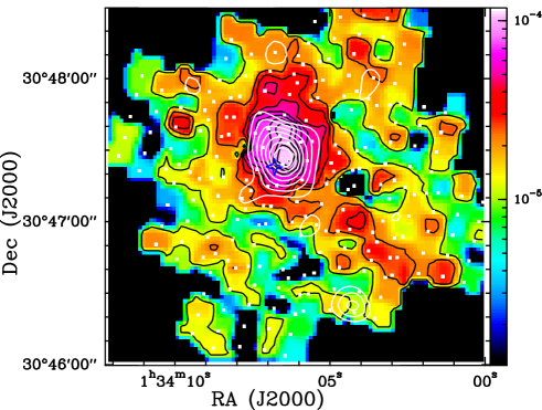
Overlays of the [C ii] map with maps of H $\alpha$ , H i, CO(2–1) and dust continuum in the MIR and FIR (MIPS 24 $\,\mu$ m, PACS 100 & 160 $\,\mu$ m) are shown in Fig. 5. The dust continuum maps correlate well with the [C ii] map. They peak towards the H ii region and show the spiral arm extending from the H ii region in south-western direction. In contrast, CO emission shows a clumpy structure wrapping around the H ii region towards the east. CO emission shows the spiral arm seen in the continuum, but its peaks are shifted towards the south. The H i emission shows a completely different morphology, peaking towards the north and south of the H ii region and showing a clumpy filament running towards the west. Further below, we will discuss the correlations in more detail.

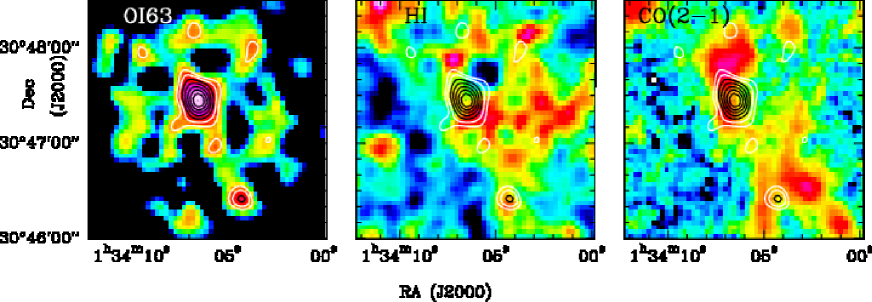
Fig. 6 shows overlays of the [O i] 63 $\,\mu$ m map at a resolution of 12″ with H i and CO(2–1). Towards the south and south-west of the H ii region, the [O i] 63 $\,\mu$ m emission matches the H i emission well. This is surprising given the high excitation requirements for the [O i] line. The secondary [O i] 63 $\,\mu$ m peak towards the south-west, is also traced by H i. It lies in between two ridges of CO emission, the arm running north-east to south-west, and a second ridge of emission running in north-south direction. The northern part of this second ridge shows an interesting layering of emission: both [O i] and H i are slightly shifted towards the east relative to this CO ridge. However, there is much less correspondence between [O i] and H i emission towards the east and north of the H ii region.

3.2 HIFI spectroscopy of the H $\alpha$ region

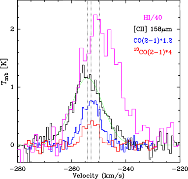
Fig. 4 shows the velocity resolved 158 $\,\mu$ m [C ii] spectrum observed with HIFI at the H $\alpha$ peak position. In addition, we show the spectra of H i and the J=2–1 transitions of CO and ¹³CO. HIFI and PACS integrated intensities agree very well. The [C ii] integrated intensity of 15.6 K km s^-1, observed with HIFI corresponds to an intensity of 1.10 $\times$ 10^-4 erg s^-1 cm^-2 sr^-1 and this matches extremely well with the [C ii] intensity observed with PACS, at the nearest PACS position, which is offset by only 3″.

All spectra are at a common resolution of $\sim 12$ ″, allowing for a detailed comparison. All spectra show a Gaussian line shape. However, the line widths are strikingly different between the atomic material traced by H i, the [C ii] line, and the molecular gas. The H i spectrum shows a FWHM of 16.5 km s^-1, that of [C ii] is 13.3 km s^-1, while CO 2–1 shows a width of only 8 km s^-1(Table 2). We take this as an indication that the H i disk along the line of sight is much thicker than the molecular disk while the material traced by [C ii] appears to lie in between. In addition, we find that the lines are not centered at the same velocity. The HI line is shifted by $+4.4$ km s^-1 relative to [C ii], while the CO lines are shifted by $+1.6$ km s^-1 relative to [C ii], confirming that all three tracers trace different components of the ISM. The shifts are significant, as the error of the Doppler corrections are much smaller, for HIFI (D.Teyssier, priv. comm.) as for the other data.

Based on lower spectral resolution (6 km s^-1) optical spectroscopy of H $\beta$ and [O iii] emission lines, the velocity of the ionized gas is deduced to be shifted by $-16.9$ km s^-1 with respect to the [C ii] line, with a velocity dispersion of 11 km s^-1 (Willner & Nelson-Patel 2002; Zaritsky et al. 1989). The optical spectroscopic data is however at much higher angular resolution (2–4″). A map of the emission lines originating solely from the ionized medium, which would allow to smooth these data to 12″ resolution for direct comparison with the other data, is not yet available. In Section 6.2, we will use PDR models to show that about 20–30% of the observed [C ii] stems from the ionized gas of the BCLMP 302 H ii region.

In summary, we find a “layering” of the line-of-sight velocities tracing the different ISM components. The velocity increases from H $\alpha$ to [C ii] to CO to H i.

Table 2: Parameters derived from Gaussian fits to spectra observed with HIFI, VLA, and IRAM 30m, at the H

\alpha

peak position (Figs. 2 & 4).

\theta_{\rm b}

indicates the half power beamwidth.

Line	$\theta_{\rm b}$	$\int{T{\rm dv}}$	$v_{\rm cen}$	$\Delta v$
	^′′	K km s^-1	km s^-1	km s^-1
[C ii]	11	15.6 $\pm$ 0.5	-254.1 $\pm$ 0.1	12.9 $\pm$ 0.9
H i	11	1446.7 $\pm$ 44.1	-249.7 $\pm$ 0.2	16.5 $\pm$ 0.6
CO (1–0)	22	3.2 $\pm$ 0.2	-252.3 $\pm$ 0.2	7.5 $\pm$ 0.5
CO (2–1)	11	5.3 $\pm$ 0.1	-252.8 $\pm$ 0.1	7.9 $\pm$ 0.3
¹³CO(1–0)	22	0.28 $\pm$ 0.02	-252.9 $\pm$ 0.2	5.8 $\pm$ 0.5
¹³CO(2–1)	11	0.69 $\pm$ 0.06	-252.8 $\pm$ 0.3	6.2 $\pm$ 0.5

3.3 Detailed comparison of [C ii] emission with other tracers

Table 3: Correlation coefficients for the scatter plots in Fig. 7.

Tracers	Correlation Coefficient
	Entire	Region	Region	Region
	Map	$A$	$B$	$C$
[C ii]–H $\alpha$	0.60	0.93	0.66	0.30
[C ii]–CO(2–1)	0.41	0.40	0.47	…
[C ii]–H i	0.22	$<0.1$	$<$ 0.10	0.14
[C ii]–[O i]	…	0.77	…	…
[C ii]–F₂₄	0.61	0.86	0.66	0.41
[C ii]–F₁₀₀	0.59	0.85	0.56	0.43

Table 4: Average values and their variation of the different tracers arising from the H ii region, the spiral arm and the region

C

Tracer	Region $A$	Region $B$	Region $C$
[C ii] (erg s^-1 cm^-2 sr^-1)	( $4.51\pm 2.30$ ) $\times 10^{-5}$	( $1.28\pm 0.48$ ) $\times 10^{-5}$	( $1.19\pm 0.42$ ) $\times 10^{-5}$
H $\alpha$ (erg s^-1)	(7.1 $\pm$ 6.9) $\times 10^{37}$	(5.3 $\pm$ 1.8) $\times 10^{36}$	(7.95 $\pm$ 1.93) $\times 10^{36}$
CO (2–1) (K km s^-1)	1.88 $\pm$ 0.98	2.95 $\pm$ 1.40	0.29 $\pm$ 0.14
H i ((K km s^-1)	1597 $\pm$ 358	1267 $\pm$ 325	620 $\pm$ 309
[O i] (erg s^-1 cm^-2 sr^-1)	(1.28 $\pm$ 0.09 $\times 10^{-5}$	…	…
F₂₄ (Jy beam^-1)	101.9 $\pm$ 82.8	32.2 $\pm$ 8.6	11.9 $\pm$ 1.50
F₁₀₀ (Jy beam^-1)	0.66 $\pm$ 0.37	0.26 $\pm$ 0.05	0.12 $\pm$ 0.03

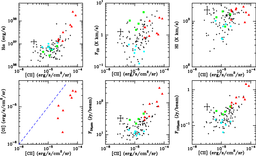
For a more quantitative estimate of the correspondence between the different tracers in which the spiral arm has been mapped we have created scatterplots of intensities of tracers like H $\alpha$ , ¹²CO, H i, [O i] 63 $\,\mu$ m, MIPS 24 $\,\mu$ m and PACS 100 $\,\mu$ m as a function of the [C ii] intensities (Fig. 7). We have used intensities from all the maps which are smoothed to a resolution of 12″ and gridded on a 12″ grid. In order to identify any apparent trends in the emission we have defined three sub-regions within the mapped region: Region $A$ corresponds to the H ii region BCLMP 302 itself, Region $B$ corresponds to the south-western more quiescent part of the spiral arm, traced by e.g. the 100 $\,\mu$ m continuum emission, and centered on a peak of CO emission, and Region $C$ lies outside of the prominent CO arm. These three sub-regions are marked by black rectangles in Figure 5. A second H ii region along the arm, lies just outside and to the north of the box defining the quiescent arm region. For the remainder of the paper we always analyze and compared the results for these three sub-regions separately.

In the log-log scatter plots of Figure 7, we find that the H $\alpha$ , [O i], and continuum emission at 24 $\,\mu$ m and 100 $\,\mu$ m show pronounced linear correlations with the [C ii] emission within the H ii region. In the region $C$ , the intensities of the H $\alpha$ emission and the continuum emission at 24 and 100 $\,\mu$ m remain almost constant. The CO(2–1) intensity in the H ii region ( $A$ ) is only poorly correlated with the [C ii] emission. In regions $B$ and $C$ the CO(2–1) intensity shows no correlation with the [C ii] intensity and has a large scatter. H i does not show any correlation with [C ii].

A more quantitative analysis of the correlation between the different tracers and [C ii], is obtained by calculating the correlation coefficient ( $r$ ) (Table 3). For the entire region H $\alpha$ and 24 $\,\mu$ m and 100 $\,\mu$ m intensities show around 60% correlation with the [C ii] intensities. For the region $A$ H $\alpha$ , [O i], 24 $\,\mu$ m, and 100 $\,\mu$ m are well correlated ( $r>0.75$ ) with [C ii]. The H $\alpha$ emission is strongly correlated with the [C ii] intensity also on the south-western arm position. The [O i]/[C ii] intensity ratio measured primarily in the H ii region varies between 0.1–0.4 and this variation is significantly larger than the estimated uncertainties.

4 [C ii] as a tracer of star formation

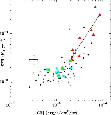
In Fig. 8, we plot the star formation rate (SFR), estimated from the 24 $\,\mu$ m MIPS data and the KPNO H $\alpha$ data, as a function of the [C ii] intensity. Positions within the selected regions $A$ , $B$ , and $C$ are marked using different symbols and colours similar to Fig. 7. The SFR has been calculated from SFR $\leavevmode\nobreak\ =\leavevmode\nobreak\ [L(H\alpha)\leavevmode\nobreak\ +\leavevmode\nobreak\ 0.031L(24)]\leavevmode\nobreak\ \times\leavevmode\nobreak\ 5.35\leavevmode\nobreak\ \times 10^{-35}$ in $\mathrm{M}_{\odot}$ yr^-1, where L(H $\alpha$ ) is the H $\alpha$ luminosity in Watt and L(24) is defined as $\nu L_{\nu}$ at 24 $\,\mu$ m in Watt (Calzetti et al. 2007). We have assumed a Kroupa (2001) initial mass function with a constant SFR over 100 Myr. Here, we study the correlation on scales of $12^{\prime\prime}$ corresponding to 50 pc. On these small scales, we may start to see a break-up of any tight correlations between the various tracers of the SFR.

Viewing at all pixels we find a steepening of the slope in the log–log plots from regions where both the SFR and [C ii] are weak, to regions where both are strong. Towards the H ii region ( $A$ ), we find an almost linear relation between $\log$ (SFR) and $\log$ ([C ii]), with a good correlation, $r=0.90$ and the fitted slope is 1.48 $\pm$ 0.26, i.e. the SFR goes as [C ii] to the power 1.48. Region $B$ shows a correlation coefficient of 0.64 and region $C$ shows no correlation.

5 Energy Balance in the spiral arm

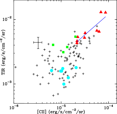
Boquien et al. (2010b) have obtained a linear fit to the total infrared (TIR) luminosity as a function of the luminosity in the PACS 160 $\,\mu$ m band for the entire M 33 galaxy. The TIR is the total infrared intensity, integrated between $1\,\mu$ m and 1 mm. It is about a factor 2 (Rubin et al. 2009) larger than the FIR continuum which is integrated between 42.7 and 122 $\mu$ m. Boquien et al. (2010b) derived the TIR from fits of Draine et al. (2007) models to the MIPS, PACS, and SPIRE FIR data. And they find a tight linear relation between the two quantities: ${\rm log}L_{\rm TIR}=a\times{\rm log}L_{160}+b$ with $a$ = 1.013 $\pm$ 0.008 and $b$ = 0.429 $\pm 0.097$ . We have used this relation to derive the TIR intensity at each position of the mapped region, at a resolution of 12″. To check that this is a valid approach, we independently derived the TIR at individual positions by fitting a greybody to the MIPS, PACS, and SPIRE data, smoothed to a common resolution of $40^{\prime\prime}$ . The resulting TIR agrees within 10% with the TIR derived from only the 160 $\,\mu$ m band.

Figure 9 shows a scatterplot between TIR and [C ii]. Positions corresponding to the selected sub-regions are indicated using different markers. We find that [C ii] and TIR are tightly correlated with a correlation coefficient of 0.87 only in the H ii region ( $A$ ) with the fitted slope being 0.64 $\pm$ 0.14. The correlation coefficient in region $B$ is 0.52 and and $C$ shows no correlation.

Incident FUV photons with energies high enough to eject electrons from dust grains (h $\nu>6$ eV) heat the gas via these photoelectrons, with a typical efficiency of 0.1–1% (Hollenbach & Tielens 1997). Efficiency is defined as the energy input to the gas divided by the total energy of the FUV photons absorbed by dust grains. Based on ISO/LWS observations of a sample of galaxies, Malhotra et al. (2001) found that (a) more than 60% of the galaxies show $L_{\rm[CII]}/L_{\rm FIR}>0.2$ % and (b) $L_{\rm[CII]}/L_{\rm FIR}$ decreases with warmer FIR colors and increasing star formation activity, indicated by higher $L_{\rm FIR}/L_{\rm B}$ ratios, where $L_{\rm B}$ is the luminosity in the B band. We have calculated the ratio of the intensities of [C ii]/TIR, as a proxy for the heating efficiency, and plotted it against with [C ii] intensities (Fig. 10). The heating efficiency vary by more than one order of magnitude within the $2^{\prime}\times 2^{\prime}$ region, between 0.07 and 1.5%. Considering an uncertainty of 20% in both the measured 160 $\,\mu$ m intensities and the [C ii] intensities, for the relation between the 160 $\,\mu$ m luminosity and the TIR luminosity mentioned earlier, we estimate the uncertainty in the [C ii]/TIR ratio to be $\sim 30$ %. The observed variation in the [C ii]/TIR intensity ratios is significantly larger than the uncertainty we estimate from the [C ii] and 160 $\,\mu$ m intensities. For the H ii region ( $A$ ), we find heating efficiencies between 0.2 and 1.0%. Regions $B$ and $C$ show efficiencies between 0.15–0.4% and 0.4–1.2%. Within the H ii region ( $A$ ), the total heating efficiency, including the [O i] 63 $\,\mu$ m line, ([C ii]+[O i])/TIR, lies between 0.3–1.2% (Fig. 10). Outside the H ii region, reliable [O i] data is largely missing.

6 Modeling the PDR emission at the H $\alpha$ peak of BCLMP 302

6.1 Estimate of FUV from TIR

One of the key parameters of PDRs is the FUV radiation field which heats the PDR. From energy considerations, the total infrared cooling emission is a measure of the irradiating FUV photons of the embedded OB stars. We estimate the FUV flux G₀ (6 eV $<h\nu<$ 13.6 eV) impinging onto the cloud surfaces from the emergent total infrared intensities: G₀ = 4 $\pi$ $I_{\rm FIR}=4\,\pi\,0.5\,I_{\rm TIR}$ with G₀ in units of the Habing field $1.6\,10^{-3}$ erg s^-1 cm^-2 (Habing 1968) and the intensity of the far-infrared continuum between $42.5\,\mu$ m and $122.5\,\mu$ m, $I_{\rm FIR}$ , in units of erg s^-1 cm^-2 sr^-1. Here, we assume that heating by photons with $\rm{h}\nu<6$ eV contributes a factor of $\sim 2$ (Tielens & Hollenbach 1985) and that the bolometric dust continuum intensity $I_{\rm TIR}$ is a factor of $\sim 2$ larger than $I_{\rm FIR}$ (Dale et al. 2001).

At the H $\alpha$ peak position, the TIR intensity of 1.18 $\times 10^{-2}$ erg s^-1 cm^-2 sr^-1 translates into a FUV field of $G_{0}=46$ in Habing units. Outside of the H $\alpha$ peak, the FUV field, estimated from the TIR, drops by more than one order of magnitude (cf. Fig. 9).

The FUV radiation leaking out of the clouds is measured using the GALEX UV data (Martin et al. 2005; Gil de Paz et al. 2007) to be G ${}_{0}=24$ for a 12″ aperture.

We thus find, that 66% of the FUV photons emitted by the OB stars of the H ii region are absorbed and re-radiated by the dust, and 34% are leaking out of the cloud, at the H $\alpha$ position. This is consistent with the FUV extinction derived from the H $\alpha$ and 24 $\,\mu$ m fluxes (Relaño & Kennicutt 2009) and the FUV/H $\alpha$ reddening curve (Calzetti 2001).

It is interesting to note that H ii regions observed in the LMC and other spiral galaxies by Oey & Kennicutt (1997) and Relaño et al. (2002) show that typically around 50% of the ionizing stellar radiation escape the H ii regions, roughly similar to the fraction of 36% we find in BCLMP 302/M33.

6.2 [C ii] emission from the ionized gas

Table 5: Properties of the H ii region BCLMP 302

Excitation parameter $u$	180 pc cm^-2	IK74
Radius $r$	39 pc	IK74
Mass	10⁵ $\mathrm{M}_{\odot}$	IK74
rms electron density	6.2 cm^-3	IK74
Electron density $n_{e}$	100 cm^-3	R08
Ionization parameter $U$	$-3.3$	this paper
Effective temperature $T_{\rm eff}$	38,000 K	this paper
H $\alpha$ luminosity	2.2 10³⁸ erg s^-1	KPNO map

²²2 As explained in the text, the value given for the electron density (

n_{e}

)is assumed to hold for BCLMP 302.\tablebib

IK74 Israel & van der Kruit (1974), R08 Rubin et al. (2008)

In Table 5 we present properties of the H ii region BCLMP 302 compiled from the literature and also calculated thereof. These properties were used to estimate the fraction of [C ii] emission contributed by this H ii region using the model calculations of Abel et al. (2005) and Abel (2006). These authors have estimated the [C ii] emission for a wide range of physical conditions in H ii regions, varying their electron density $n_{e}$ , ionization parameter $U$ , and effective temperature $T_{\rm eff}$ .

The [C ii] PACS map is centered on the bright H ii region BCLMP302 (Boulesteix et al. 1974), which corresponds to the H ii region no. 53 in the M33 catalog of Israel & van der Kruit (1974, IK74). Using the measured radio flux and the formula $u({\rm pc\leavevmode\nobreak\ cm}^{-2})=13.5(S/{\rm f.u.})^{1/3}(D/{\rm kpc})^{2/3}$ (Israel et al. 1973), IK74 estimate the excitation parameter $u=180$ pc cm^-2 for a distance of 720 kpc. IK74 also derive an rms electron density of 6.2 cm^-3, and estimate the radius $r$ of the H ii region to be 38.5 pc. We did not correct these results for the now better known distance, as it does not affect our conclusions. For an electron temperature $T_{e}$ of 10,000 K, Panagia (1973) expresses the excitation parameter as $u({\rm pc\leavevmode\nobreak\ cm}^{-2})=2.2\times 10^{-19}\left[{N(L)}{(\beta-\beta_{1})^{-1}}\right]^{1/3}$ , where ( $\beta$ - $\beta_{1}$ ) is the recombination rate to the excited levels of hydrogen in units of cm³ s^-1. Thus we get for the total flux of ionizing photons $N(L)=4.6\,10^{43}\,u^{3}$ s^-1. Using the above values of the parameters, the dimensionless ionization parameter $U$ was derived via $U=N(L)/(c\,4\,\pi\,r^{2}\,n_{\rm H+})$ (Evans & Dopita 1985; Morisset 2004).

The rms electron density derived by IK74, provides only a lower limit to the true electron density and observations of e.g. the [S ii] doublet at 6754 Å are missing which would allow a direct estimate. Rubin et al. (2008) observed 25 H ii regions in M33 using Spitzer-IRS, and concluded that their electron densities are $\sim 100$ cm^-3. Since there is no apparent reason for the $n_{e}$ in BCLMP 302 to be significantly different, we assume $n_{e}=100$ cm^-3. Hence, with $n_{\rm H+}=n_{e}$ , we estimate $\log U=-3.3$ (Table 5).

The observed ratio of double and single ionized Nitrogen, [N iii] 57 $\,\mu$ m/[N ii] 122 $\,\mu$ m, at the H $\alpha$ position (Table 1), indicates an effective temperature of the ionizing stars of about 38,000 K (Rubin et al. 1994).

From the model calculations of Abel (2006, Fig. 5), we estimate the fraction of [C ii] emission from the BCLMP 302 H ii region. The [C ii] fraction increases with dropping electron density, but is only weakly dependent on the ionization parameter and the stellar continuum model. Depending on the model, the resulting fraction varies slightly, $\sim 20-30$ %. The fraction would drop to about 10%, for an electron density of $10^{3}$ cm^-3.

Observations of the [N ii] 205 $\,\mu$ m line, in addition to the 122 $\,\mu$ m line would allow to estimate more accurately the electron density of the H ii region. The model calculations and observations compiled by Abel (2006) show that the [C ii] intensities stemming from H ii regions and the intensities of the [N ii] 205 $\,\mu$ m line are tightly correlated. Abel (2006) find $\mathrm{Log}\left[I^{\mathrm{C^{+}}}_{\mathrm{H^{+}}}\right]=0.937\mathrm{Log}\left[I^{\mathrm{NII}}_{\mathrm{H^{+}}}\right]+0.689$ (erg cm^-2 s^-1). Assuming that 30% of [C ii] emission stems from the BCLMP 302 H ii region at the H $\alpha$ peak position, we estimate a [N ii] 205 $\,\mu$ m intensity of $\sim 3.6\times 10^{-6}$ erg s^-1 cm^-2 sr^-1 (cf. Table 1), corresponding to $3\times 10^{-18}$ W m^-2. The expected [N ii] 205 $\,\mu$ m intensity is a factor of 3 below the estimated rms of our PACS observations and hence is consistent with the non-detection. Using the detected [N ii] 122 $\,\mu$ m line, and the predicted [N ii] 205 $\,\mu$ m intensity from above, the [N ii] 122 $\,\mu$ m/[N ii] 205 $\,\mu$ m ratio is 2.8 and this corresponds to an $n_{e}$ of $10^{2}$ cm^-3 (Abel et al. 2005, Fig. 22), which is consistent with the $n_{e}$ assumed by us for the above calculations.

6.3 Comparison with PDR models

Table 6: Input to the PDR model for the HIFI position

Tracer	Intensity
[C ii]^∗	8.4 10^-5
[O i]	3.0 10^-5
CO (1–0)^∗∗	7.5 10^-9
CO (2–1)	6.7 10^-8
TIR	1.18 10^-2

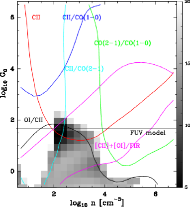
³³3All intensities are in units of erg sec^-1cm^-2 sr^-1. ^∗ The observed [C ii] intensities was multiplied by 0.7, assuming that 30% of the emission stems from the H ii region. ^∗∗ The CO 1–0 data at 22″ resolution were multiplied by the beamfilling factor 1.5, estimated by smoothing the 2–1 data from 11″ to 22″ resolution.

Here we investigate whether the FIR and millimeter lines, together with the TIR, observed towards the H $\alpha$ peak, can be consistently explained in terms of emission from the PDRs at the surfaces of the molecular clouds. We use the line and total infrared continuum intensities at a common resolution of 12″.

At the position of the H $\alpha$ peak we observe the following intensity ratios on the erg scale (cf. Table 6) [O i]/[C ii] = 0.35, [C ii]/CO(1–0) = 1.1 $\times 10^{4}$ , [C ii]/CO(2–1) = 1263, ([C ii]+[O i])/TIR = 9.6 $\times 10^{-3}$ and CO(2–1)/CO(1–0) = 8.8. Comparing all ratios with the PDR model of Kaufman et al. (1999) (Fig. 11), we find a best fitting solution near a FUV field of G₀=32 in units of the Habing field and a density of 320 cm^-3. The fitted FUV field agrees rather well with the FUV field of G ${}_{0}=46$ (in Habing units) estimated from the TIR continuum. The corresponding reduced $\chi^{2}$ was estimated assuming an error of 30% on the observed intensity ratios. The reduced $\chi^{2}$ is defined as $\chi^{2}=1/(n-2)(\sum\limits_{i=0}^{n}{(I_{i}^{obs}-I_{i}^{model})^{2}}/\sigma_{i}^{2}$ ), where $(n-2)$ is the number of degrees of freedom with $n$ being the number of observed quantities used for the fitting and $I$ denotes either integrated intensities or ratios of integrated intensities. We find the minimum value of $\chi^{2}$ to be 4.4, indicating that the fit is not satisfactory. Indeed, the fitted density seems rather low, given the high critical densities of the [C ii] and in particular also of the [O i] line. On the other hand, the observed [O i]/[C ii] ratio, is consistent with the low density solution. The ratios with the CO lines, deviate from this solution. For instance, the CO 2–1/1–0 ratio together with the derived FUV, indicates a higher density of about $10^{4}$ cm^-3. Using line ratios to compare with the PDR model, allows to ignore beam filling effects, to first order. Note that the absolute [C ii] intensity, reduced by the fraction of 30% stemming from the H ii region, agrees well with the best fitting solution, indicating a [C ii] beam filling factor of about 1.

The rather poor fit of the intensity ratios towards the H $\alpha$ peak shows the short comings of a plane-parallel single density PDR model. First tests using KOSMA- $\tau$ PDR models Röllig et al. (2006) of spherical clumps with density gradients reconcile better to the observations. This indicates strong density gradients along the line of sight. In a second paper, we shall include new HIFI [C ii] data along two cuts through the BCLMP 302 region and explore detailed PDR models, which include the effects of geometry and sub-solar metallicity.

7 Discussion

Mapping observations of the northern inner arm of M 33 at an unprecedented spatial resolution of 50 pc have revealed details of the distribution of the various components of the interstellar medium and their contribution to the [C ii] emission. [C ii] at 158 $\mu$ m is one of the major cooling lines of the interstellar gas. Thus irrespective of whether hydrogen is atomic or molecular, the [C ii] line emission is expected to be strong wherever there is warm and photodissociated gas. We have identified emission towards the H ii region as well as from the spiral arm seen in the continuum, and from a region outside of the well-defined spiral arm. [C ii] emission is strongly correlated with the H $\alpha$ and dust continuum emission, while there is little correlation with CO, and even less with H i. This suggests that the cold neutral medium (CNM; Wolfire et al. 1995) does not contribute significantly to the [C ii] emission in the BCLMP 302 region. Recently, Langer et al. (2010) found a similar poor correlation between [C ii] and H i emission in a sample of 29 diffuse clouds using HIFI. The lack of correlation between [C ii] and CO found in BCLMP 302, may indicate that significant parts of the molecular gas are not traced by CO because it is photo-dissociated in the low-metallicity environment of M33. This interpretation is consistent with both theoretical models developed by Bolatto et al. (1999) and recent observational studies of diffuse clouds in the Milky Way by Langer et al. (2010), and of dwarf galaxies by Madden et al. (2011).

Comparison of the first velocity-resolved [C ii] spectrum of M33 (at the H $\alpha$ peak of BCLMP 302) with CO line profiles show that the [C ii] profile is much broader, by a factor of $\sim 1.6$ , and slightly shifted in velocity, by $\sim 1.6$ km s^-1. Compared to the H i line, at the same angular resolution, the [C ii] line is less broad by a factor $\sim 1.3$ and shifted by $\sim 4.4$ km s^-1. These findings indicate that the [C ii] line is not completely mixed with the CO emitting gas, but rather traces a different more turbulent outer layer of gas with slightly different systemic velocities, which is associated with the ionized gas.

Interestingly, recent [C ii] HIFI observations of Galactic star forming regions (Ossenkopf et al. 2010; Joblin et al. 2010) also show broadened and slightly shifted [C ii] line profiles relative to CO.

The two major cooling lines of PDRs are the [O i] line at 63 $\mu$ m and the [C ii] 158 $\mu$ m line. The intensity ratios [OI]/[CII] and ([OI]+[CII]) vs. the TIR continuum, have been used extensively to estimate the density and FUV field of the emitting regions. Using ISO/LWS, Higdon et al. (2003) observed the far-infrared spectra of the nucleus and six giant H ii regions in M 33, not including BCLMP 302, but including NGC 604, IC 142, and NGC 595 shown in Figure 1. The 70″ ISO/LWS beam corresponds to 285 pc and therefore samples a mixture of the different ISM phases. They find [O i]/[C ii] line ratios in the range 0.7 to 1.3, similar to the range of values found in the center and spiral arm positions of M83 and M51 (Kramer et al. 2005). Towards the H ii region BCLMP 302 in the northern inner arm of M 33, we measure much lower [O i]/[C ii] ratios between 0.1–0.4. These ratios lie towards the lower end of the values found by Malhotra et al. (2001) in their ISO/LWS study of the unresolved emission of 60 galaxies who find values between $\sim 0.2$ and 2. Similarly low values of down to 0.16 are found e.g. in the Galactic star forming regions DR 21 and W3 IRS5 (Jakob et al. 2007; Kramer et al. 2004). Comparison with the PDR models of Kaufman et al. (1999, Fig. 4) and Röllig et al. (2006) show that the [O i] 63 $\,\mu$ m line becomes stronger than the [C ii] emission in regions of high densities of more than about $10^{4}$ cm^-3. At the H $\alpha$ peak position in BCLMP 302, we observed a ratio of 0.4, after correcting [C ii] for the contribution from the ionized gas. This ratio indicates lower densities and a FUV field of less than about 100 G₀ (cf. Fig. 11). Still lower ratios, indicate lower impinging FUV fields.

The ratio of [O i] +[C ii] emission over the FIR continuum, is a good measure of the total cooling of the gas relative to the cooling of the dust, reflecting the ratio of FUV energy heating the gas to the FUV energy heating the grains, and hence the grain heating efficiency, i.e. the efficiency of the photo-electric (PE) effect (Rubin et al. 2009). Efficiencies of up to about 5% are still consistent with FUV heating, i.e. with emission from PDRs (Bakes & Tielens 1994; Kaufman et al. 1999). The PE heating efficiency is a function of FUV field, electron density, and temperature. A high FUV field leads to a large fraction of ionized dust particles, lowering the efficiency. On the other hand, low metallicities naturally lead to increased efficiencies as e.g. the PDRs become larger when the dust attenuation is lowered (Rubin et al. 2009).

Higdon et al. (2003) compared the [O i]+[C ii] emission with the FIR(LWS) continuum integrated between 43 and 197 $\,\mu$ m, and obtained ratios of 0.2% to 0.7%, corresponding to 0.4 to 1.4% for a rough estimate of the FIR/TIR conversion factor of 2 (Dale et al. 2001; Rubin et al. 2009). Towards the $2^{\prime}\times 2^{\prime}$ region presented here, the [C ii]/TIR ratio varies by more than a factor 10 between 0.07 and 1.5%. Extra galactic observations at resolutions of 1 kpc or more, find efficiencies of only up to $\sim 0.3$ % (Kramer et al. 2005; Malhotra et al. 2001). The observations of M 31 by Rodriguez-Fernandez et al. (2006) with ISO/LWS at $\sim 300$ pc resolution, do also find high efficiencies of up to 2%. Rubin et al. (2009) analyzed BICE [C ii] maps of the LMC at 225 pc resolution, and find efficiencies of upto 4% in this low metallicity environment. The mean values found in the LMC are however much lower: 0.8% in the diffuse regions, dropping to $\sim 0.4$ % in the SF regions. A similar variation was found in the Galactic plane observations by Nakagawa et al. (1998). Heating efficiencies observed in the Milky Way span about two orders of magnitude. Habart et al. (2001) observed efficiencies as high as 3% in the low-UV irradiated Galactic PDR L1721, whereas Vastel et al. (2001) also using ISO/LWS fluxes of [C ii] and [O i], found a very low heating efficiency of 0.01% in W49N. The global value for the Milky Way from COBE observations is $\sim 0.15\%$ (Wright et al. 1991). The galactic averages observed by e.g. Malhotra et al. (2001), are dominated by bright emission from the nuclei where the SFR and the FUV fields are large, hence lowering the photo-electric heating efficiencies.

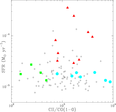
Unresolved observations of external galaxies find a tight correlation between CO and [C ii] emission. This was initially seen by Stacey et al. (1991) with the KAO, and subsequently supported by ISO/LWS observations. However at spatial scales of 50 pc we do not detect such a tight correlation in BCLMP 302. This lack of correlation between CO and [C ii] emission is already seen in the maps of spiral arms in M 31 at $\sim 300$ pc resolution (Rodriguez-Fernandez et al. 2006). As summarized by them, the [C ii]/CO(1–0) ratio varies from $\sim 1300$ in galactic disks to about 6000 in starbursts and to about 23,000 in the LMC. In BCLMP 302/M 33, we find that the [C ii]/CO(1–0) ratio varies between 200 to 6000, with the H ii region having values between 800-5000 (Fig. 12). The region $C$ shows large values of the [C ii]/CO(1–0) intensity ratios as CO is hardly detected. Thus, while the [C ii]/CO(1–0) intensity ratios are higher for regions with high SFRs, there is no marked correlation between the two quantities at scales below about 300 pc. The tight correlation between [C ii] and CO emission breaks down at scales resolving the spiral arms of galaxies.

References

Abel et al. (2005) Abel, N. P., Ferland, G. J., Shaw, G., & van Hoof, P. A. M. 2005, ApJS, 161, 65
Abel (2006) Abel, N. P. 2006, MNRAS, 368, 1949
Asplund et al. (2009) Asplund, M., Grevesse, N., Sauval, A.J., Scott, P. 2009, ARA&A, 47, 481
Bakes & Tielens (1994) Bakes, E. L. O., Tielens, A. G. G. M. 1994, ApJ, 427, 822
Beirão et al. (2010) Beirão, P., et al. 2010, A&A, 518, L60
Bolatto et al. (1999) Bolatto, A. D., Jackson, J. M., & Ingalls, J. G. 1999, ApJ, 513, 275
Boquien et al. (2010a) Boquien, M., et al. 2010, A&A, 518, L70
Boquien et al. (2010b) Boquien, M., et al. 2010 (in preparation)
Boulesteix et al. (1974) Boulesteix, J., Courtes, G., Laval, A., Monnet, G., & Petit, H. 1974, A&A, 37, 33
Calzetti et al. (2007) Calzetti, D., et al. 2007, ApJ, 666, 870
Calzetti (2001) Calzetti, D. 2001, PASP, 113, 1449
Contursi et al. (2002) Contursi, A., et al. 2002, AJ, 124, 751
Cooksy et al. (1986) Cooksy, A.L., Blake, G.A., Saykally, J. 1986, ApJ, 305, 89
Crawford et al. (1985) Crawford, M. K., Genzel, R., Townes, C. H., & Watson, D. M. 1985, ApJ, 291, 755
Dale et al. (2001) Dale, D. A., Helou, G., Contursi, A., Silbermann, N.A., Kolhatkar, S. 2001, ApJ, 549, 215
Draine et al. (2007) Draine, B.T., Li, A. 2007, ApJ, 657, 810
Evans & Dopita (1985) Evans, I. N., & Dopita, M. A. 1985, ApJS, 58, 125
Ferland et al. (1998) Ferland, G. J., Korista, K. T., Verner, D. A., Ferguson, J. W., Kingdon, J. B., & Verner, E. M. 1998, PASP, 110, 761
Freedman et al. (1991) Freedman, W. L., Wilson, C. D., & Madore, B. F. 1991, ApJ, 372, 455
Gil de Paz et al. (2007) Gil de Paz, A., et al. 2007, ApJS, 173, 185
Gratier et al. (2010) Gratier, P., et al. 2010, A&A, 522, A3
Gry et al. (2003) Gry, C., Swinyard, B., Harwood, A., et al. 2003, ’The ISO Handbook’, Volume III - LWS - The Long Wavelength Spectrometer Version 2.1 (June, 2003). Series edited by T.G. Mueller, J.A.D.L. Blommaert, and P. Garcia-Lario. ESA SP-1262, ISBN No. 92-9092-968-5, ISSN No. 0379-6566. European Space Agency, 2003.
Habart et al. (2001) Habart, E., Verstraete, L., Boulanger, F., et al. 2001, A&A, 373, 702
Habing (1968) Habing, H. J. 1968, Bull. Astron. Inst. Netherlands, 19, 421
Heiles (1994) Heiles, C. 1994, ApJ, 436, 720
Higdon et al. (2003) Higdon, S. J. U., Higdon, J. L., van der Hulst, J. M., & Stacey, G. J. 2003, ApJ, 592, 161
Hollenbach & Tielens (1997) Hollenbach, D. J., & Tielens, A. G. G. M. 1997, ARA&A, 35, 179
Hoopes & Walterbos (2000) Hoopes, C. G. & Walterbos, R. A. M. 2000, ApJ, 541, 597
Israel et al. (1973) Israel, F. P., Habing, H. J., & de Jong, T. 1973, A&A, 27, 143
Israel & van der Kruit (1974) Israel, F. P., & van der Kruit, P. C. 1974, A&A, 32, 363 (IK74)
Israel et al. (1996) Israel, F. P., Maloney, P. R., Geis, N., Herrmann, F., Madden, S. C., Poglitsch, A., Stacey, G. J. 1996, ApJ, 465, 738
Jakob et al. (2007) Jakob, H., Kramer, C., Simon, R., Schneider, N., Ossenkopf, V., Bontemps, S., Graf, U. U., & Stutzki, J. 2007, A&A, 461, 999
Joblin et al. (2010) Joblin, C., et al. 2010, A&A, 521, L25
Kaufman et al. (1999) Kaufman, M. J., Wolfire, M. G., Hollenbach, D. J., & Luhman, M. L. 1999, ApJ, 527, 795
Kramer et al. (2004) Kramer, C., Jakob, H., Mookerjea, B., Schneider, N., Brüll, M., & Stutzki, J. 2004, A&A, 424, 887
Kramer et al. (2005) Kramer, C., Mookerjea, B., Bayet, E., Garcia-Burillo, S., Gerin, M., Israel, F. P., Stutzki, J., & Wouterloot, J. G. A. 2005, A&A, 441, 961
Kramer et al. (2010) Kramer, C., et al. 2010, A&A, 518, L67
Kroupa (2001) Kroupa, P. 2001, MNRAS, 322, 231
Langer et al. (2010) Langer, W.D., Velusamy, T., Pineda, J.L., Goldsmith, P.F., Li, D., Yorke, H.W. 2010, A&A, 521, L17
Madden et al. (1993) Madden, S. C., Geis, N., Genzel, R., Herrmann, F., Jackson, J., Poglitsch, A., Stacey, G. J., & Townes, C. H. 1993, ApJ, 407, 579
Madden et al. (2011) Madden, S. C., et al. 2011, arXiv:1105.1006
Malhotra et al. (2001) Malhotra, S., et al. 2001, ApJ, 561, 766
Martin et al. (2005) Martin, D. C., et al. 2005, ApJ, 619, L1
Morisset (2004) Morisset, C. 2004, ApJ, 601, 858
Nakagawa et al. (1998) Nakagawa, T. et al. 1998, ApJ, 115, 259
Nikola et al. (2001) Nikola, T., Geis, N., Herrmann, F., Madden, S. C., Poglitsch, A., Stacey, G. J., & Townes, C. H. 2001, ApJ, 561, 203
Oey & Kennicutt (1997) Oey, M. S., & Kennicutt, R. C., Jr. 1997, MNRAS, 291, 827
Olberg (2010) Olberg, M. 2010 “Beam observations towards Mars”, Technical Note, ICC, Vers.1.1, 2010-11-17
Ossenkopf et al. (2010) Ossenkopf, V., et al. 2010, A&A, 518, L79
Ott et al. (2010) Ott S., 2010, in ASP conference series Astronomical Data analysis Software and Systems XIX, Y. Mizumoto, K. I. Morita and M. Ohishi eds., in press
Panagia (1973) Panagia, N. 1973, AJ, 78, 929
Poglitsch et al. (2010) Poglitsch, A., et al. 2010, A&A, 518, L2
Regan & Vogel (1994) Regan, M. W., & Vogel, S. N. 1994, ApJ, 434, 536
Relaño et al. (2002) Relaño, M., Peimbert, M., & Beckman, J. 2002, ApJ, 564, 704
Relaño & Kennicutt (2009) Relaño, M., & Kennicutt, R. C. 2009, ApJ, 699, 1125
Rodriguez-Fernandez et al. (2006) Rodriguez-Fernandez, N. J., Braine, J., Brouillet, N., & Combes, F. 2006, A&A, 453, 77
Röllig et al. (2006) Röllig, M., Ossenkopf, V., Jeyakumar, S., Stutzki, J., & Sternberg, A. 2006, A&A, 451, 917
Röllig et al. (2007) Röllig, M., Abel, N. P., Bell, T. et al. 2007, A&A, 26, 467
Rubin et al. (1994) Rubin, R. H., Simpson, J. P., Lord, S. D., Colgan, S. W. J., Erickson, E. F., & Haas, M. R. 1994, ApJ, 420, 772
Rubin et al. (2008) Rubin, R. H., et al. 2008, MNRAS, 387, 45 (R08)
Rubin et al. (2009) Rubin, D., et al. 2009, A&A, 494, 647
Stacey et al. (1991) Stacey, G. J., Geis, N., Genzel, R., Lugten, J. B., Poglitsch, A., Sternberg, A., & Townes, C. H. 1991, ApJ, 373, 423
Tabatabaei et al. (2007) Tabatabaei, F. S., et al. 2007, A&A, 466, 509
Tielens & Hollenbach (1985) Tielens, A. G. G. M., & Hollenbach, D. 1985, ApJ, 291, 722
Vastel et al. (2001) Vastel, C., Spaans, M., Ceccarelli, C., Tielens, A. G. G. M., & Caux, E. 2001, A&A, 376, 1064
Verley et al. (2010) Verley, S., et al. 2010, A&A, 518, L68
Willner & Nelson-Patel (2002) Willner, S. P., & Nelson-Patel, K. 2002, ApJ, 568, 679
Wolfire et al. (1990) Wolfire, M. G., Tielens, A. G. G. M., & Hollenbach, D. 1990, ApJ, 358, 116
Wolfire et al. (1995) Wolfire, M. G., Hollenbach, D., McKee, C. F., Tielens, A. G. G. M., & Bakes, E. L. O. 1995, ApJ, 443, 152
Wright et al. (1991) Wright, E. L., Mather, J. C., Bennett, C. L. et al. 1991, ApJ, 381, 200
Zaritsky et al. (1989) Zaritsky, D., Olszewski, E. W., Schommer, R. A., Peterson, R. C., & Aaronson, M. 1989, ApJ, 345, 759

The Herschel M33 extended survey (HerM33es): PACS spectroscopy of the star forming region BCLMP 302 ††thanks: Herschel is an ESA space observatory with science instruments provided by European-led Principal Investigator consortia and with important participation from NASA.