Running coupling corrections to inclusive gluon production

Abstract

We calculate running coupling corrections for the lowest-order gluon production cross section in high energy hadronic and nuclear scattering using the BLM scale-setting prescription. At leading order there are three powers of fixed coupling; in our final answer, these three couplings are replaced by seven factors of running coupling: five in the numerator and two in the denominator, forming a ‘septumvirate’ of running couplings, analogous to the ‘triumvirate’ of running couplings found earlier for the small-$x$ BFKL/BK/JIMWLK evolution equations. It is interesting to note that the two running couplings in the denominator of the ‘septumvirate’ run with complex-valued momentum scales, which are complex conjugates of each other, such that the production cross section is indeed real. We use our lowest-order result to conjecture how running coupling corrections may enter the full fixed-coupling $k_{T}$-factorization formula for gluon production which includes non-linear small-$x$ evolution.

1 Introduction

This proceedings contribution is based on [1].

While an exact analytic formula for gluon production in $AA$ collisions in the Color Glass Condensate (CGC) framework is still not known, we do know that in $pp$ and $pA$ collisions gluon production at the level of classical gluon fields and leading-$\ln 1/x$ nonlinear quantum evolution is given by the $k_{T}$-factorization formula [2, 3]:

$$\frac{d\sigma}{d^{2}k_{T}\,dy}\,=\,\frac{2\,\alpha_{s}}{C_{F}}\,\frac{1}{{\bm{k}}^{2}}\,\int d^{2}q\,\phi_{p}({\bm{q}},y)\,\phi_{A}({{\bm{k}}-\bm{q}},Y-y).$$ (1)

Here $Y$ is the total rapidity interval of the collision, $C_{F}=(N_{c}^{2}-1)/2N_{c}$, boldface variables denote two-component transverse plane vectors ${\bm{k}}=(k^{1},k^{2})$, and $\phi_{p}$, $\phi_{A}$ are the unintegrated gluon distributions in the proton and the nucleus, respectively, which are defined by [2]

$$\phi_{A}({\bm{k}},y)\,=\,\frac{C_{F}}{\alpha_{s}\,(2\pi)^{3}}\,\int d^{2}b\,d^{2}r\,e^{-i{\bm{k}}\cdot{\bm{r}}}\ \nabla^{2}_{r}\,N_{G}({\bm{r}},{\bm{b}},y)$$ (2)

and

$$\phi_{p}({\bm{k}},y)\,=\,\frac{C_{F}}{\alpha_{s}\,(2\pi)^{3}}\,\int d^{2}b\,d^{2}r\,e^{-i{\bm{k}}\cdot{\bm{r}}}\ \nabla^{2}_{r}\,n_{G}({\bm{r}},{\bm{b}},y).$$ (3)

In Eq. (2) the quantity $N_{G}({\bm{r}},{\bm{b}},y)$ denotes the forward scattering amplitude for a gluon dipole of transverse size $\bm{r}$ with its center located at the impact parameter $\bm{b}$ scattering on a target nucleus with total rapidity interval $y$. $N_{G}({\bm{r}},{\bm{b}},y)$ can, in general, be found from the JIMWLK evolution equation. In the large-$N_{c}$ limit it is related to the quark dipole forward scattering amplitude on the same nucleus $N({\bm{r}},{\bm{b}},y)$ by

$$N_{G}({\bm{r}},{\bm{b}},y)\,=\,2\,N({\bm{r}},{\bm{b}},y)-N({\bm{r}},{\bm{b}},y)^{2},$$ (4)

where $N({\bm{r}},{\bm{b}},y)$ can be found from the BK evolution equation. The quantity $n_{G}({\bm{r}},{\bm{b}},y)$ from Eq. (3) is also a gluon dipole amplitude, but taken in a dilute regime, where it is found by solving the linear Balitsky-Fadin-Kuraev-Lipatov (BFKL) evolution equation.

Eq. (1) for the gluon production was derived in the fixed coupling approximation. However, the dipole amplitudes $N({\bm{r}},{\bm{b}},y)$, $N_{G}({\bm{r}},{\bm{b}},y)$ and $n_{G}({\bm{r}},{\bm{b}},y)$ are now known for the running coupling case due to the completion of the running coupling calculations for the BFKL/BK/JIMWLK evolution equations [4, 5]. Using the running-coupling BK (rcBK) equation, the calculational framework presented above, when applied to heavy ion collisions by replacing $\phi_{p}\rightarrow\phi_{A}$ in Eq. (1), and implemented with a careful inclusion of the nuclear geometry fluctuations, led to the prediction made in [6] of the charged particle multiplicity as a function of the collision centrality for the LHC. This prediction was confirmed by the ALICE data in [7]. However, at the time the prediction [6] was made, the scales of the couplings explicitly shown in Eqs. (1), (2), and (3) were not known and had to be modeled. Our goal here is to fix the scales of those couplings for the lowest-order gluon production.

2 Running coupling corrections: strategy

To include running coupling corrections we follow the BLM scale-setting procedure [8], which is known to be correct at least at the leading order in $1/N_{c}^{2}$. One first needs to resum the contribution of all quark bubble corrections giving powers of $\alpha_{\mu}\,N_{f}$, with $N_{f}$ the number of quark flavors and $\alpha_{\mu}$ the physical coupling at some arbitrary renormalization scale $\mu$. We then complete $N_{f}$ to the full beta-function by replacing

$$N_{f}\rightarrow-6\,\pi\,\beta_{2}$$ (5)

in the obtained expression. Here

$$\beta_{2}=\frac{11N_{c}-2N_{f}}{12\,\pi}$$ (6)

is the one-loop QCD beta-function. After this, the powers of $\alpha_{\mu}\,\beta_{2}$ should combine into physical running couplings

$$\alpha_{s}(Q^{2})\,=\,\frac{\alpha_{\mu}}{1+\alpha_{\mu}\,\beta_{2}\,\ln\frac{Q^{2}}{\mu^{2}}}$$ (7)

at various momentum scales $Q$ which would follow from this calculation. We use the $\overline{\mbox{M}S}$ renormalization scheme.

As was originally argued in [9], including running coupling corrections into the diagrams of Fig. 1 below assuming that only a gluon can be produced in the final state would leave one factor of the coupling at an arbitrary renormalization scale $\mu$. Following [9] we rectify the problem by redefining the gluon production cross-section to include production of collinear gluon–gluon and quark–anti-quark pairs with the invariant mass lower than some collinear IR cutoff $\Lambda_{coll}^{2}$. This new observable is completely $\mu$-independent and expressible in terms of the running coupling constants.

3 Running coupling corrections to LO gluon production

Gluon production at the lowest order in the coupling is shown in Fig. 1 in the $A^{+}=0$ light-cone gauge. At this order the unintegrated gluon distribution is

$$\phi({\bm{k}},y)\,=\,\frac{\alpha_{s}\,C_{F}}{\pi}\,\frac{1}{{\bm{k}}^{2}}.$$ (8)

such that Eq. (1) reduces to

$$\frac{d\sigma}{d^{2}k_{T}\,dy}\,=\,\frac{2\,\alpha_{s}^{3}\,C_{F}}{\pi^{2}}\,\frac{1}{{\bm{k}}^{2}}\,\int\,\frac{d^{2}q}{{\bm{q}}^{2}\,({\bm{k}}-{\bm{q}})^{2}}.$$ (9)

Our goal is to set the scales for the three couplings in Eq. (9).

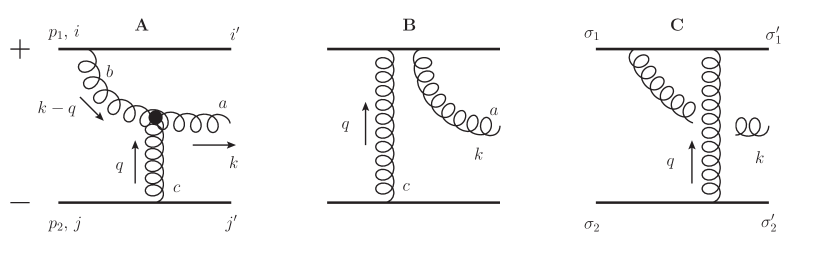
Figure 1: Diagrams contributing to the lowest-order gluon production in quark-quark scattering at high energy in the $A^{+}=0$ light-cone gauge.

The final result for the lowest-order gluon production cross section with the running coupling corrections included is [1]

$$\frac{d\sigma}{d^{2}k_{T}\,dy}\,=\,\frac{2\,C_{F}}{\pi^{2}}\,\frac{\alpha_{s}\left(\Lambda_{coll}^{2}\right)}{{\bm{k}}^{2}}\,\int\frac{d^{2}q}{{\bm{q}}^{2}\,({\bm{k}}-{\bm{q}})^{2}}\,\frac{\alpha_{s}^{2}\left({\bm{q}}^{2}\right)\,\alpha_{s}^{2}\left(({\bm{k}}-{\bm{q}})^{2}\right)}{\alpha_{s}\left(Q^{2}\right)\,\alpha_{s}\left(Q^{*\,2}\right)}$$ (10)

with the momentum scale $Q$ being a complicated function of ${\bm{q}}$ and ${\bm{k}}-{\bm{q}}$ given in [1]. An interesting feature is that the scale $Q^{2}$ is complex-valued! The cross-section (10) is, of course, real, as it contains a complex-valued coupling constant multiplied by its conjugate, $\alpha_{s}\left(Q^{2}\right)\,\alpha_{s}\left(Q^{*\,2}\right)$. Eq. (10) clearly looks like the fixed-coupling cross-section (9) with three factors of fixed-coupling replaced by the seven running couplings: we chose to refer to this structure as the septumvirate of couplings [1].

An important feature of the scale $Q$ is that in the $\bm{q}\rightarrow 0$ (or $\bm{q}\rightarrow\bm{k}$) limit

$$\ln\frac{Q^{2}}{\mu_{\overline{MS}}^{2}}\,=\,\ln\frac{{\bm{k}}^{2}}{\mu_{\overline{MS}}^{2}}+\frac{1}{2}$$ (11)

reducing Eq. (10) to

$$\frac{d\sigma}{d^{2}k_{T}\,dy}\,\approx\,\frac{4\,C_{F}}{\pi}\,\frac{\alpha_{s}\left(\Lambda_{coll}^{2}\right)\,\alpha_{s}({\bm{k}}^{2})\,\alpha_{s}(Q_{s}^{2})}{\left({\bm{k}}^{2}\right)^{2}}\,\ln\frac{{\bm{k}}^{2}}{Q_{s}^{2}}.$$ (12)

4 Ansatz for the running coupling corrections in the $k_{T}$-factorization formula

Using the lowest-order expression (10) we would like to conjecture the following running-coupling generalization of Eq. (1):

$$\frac{d\sigma}{d^{2}k_{T}\,dy}\,=\,\frac{2\,C_{F}}{\pi^{2}}\,\frac{1}{{\bm{k}}^{2}}\int d^{2}q\ {\overline{\phi}}_{p}({\bm{q}},y)\,{\overline{\phi}}_{A}({\bm{k}}-{\bm{q}},Y-y)\,\frac{\alpha_{s}\left(\Lambda_{coll}^{2}\right)}{\alpha_{s}\left(Q^{2}\right)\,\alpha_{s}\left(Q^{*\,2}\right)}$$ (13)

with the new (rescaled) distribution functions defined by (cf. Eqs. (2) and (3))

$${\overline{\phi}}_{A}({\bm{k}},y)\,=\,\frac{C_{F}}{(2\pi)^{3}}\,\int d^{2}b\,d^{2}r\,e^{-i{\bm{k}}\cdot{\bm{r}}}\ \nabla^{2}_{r}\,N_{G}({\bm{r}},{\bm{b}},y)$$ (14)

and

$${\overline{\phi}}_{p}({\bm{k}},y)\,=\,\frac{C_{F}}{(2\pi)^{3}}\,\int d^{2}b\,d^{2}r\,e^{-i{\bm{k}}\cdot{\bm{r}}}\ \nabla^{2}_{r}\,n_{G}({\bm{r}},{\bm{b}},y).$$ (15)

One may use this ansatz, along with $N_{G}$ obtained from the rcBK evolution to further improve the existing CGC phenomenology for particle multiplicity along with its centrality and rapidity dependence at RHIC and LHC.

References

References

- [1] W. A. Horowitz and Yuri V. Kovchegov. Running Coupling Corrections to High Energy Inclusive Gluon Production. Nucl. Phys., A849:72–97, 2011.
- [2] Yuri V. Kovchegov and Kirill Tuchin. Inclusive gluon production in DIS at high parton density. Phys. Rev., D65:074026, 2002.
- [3] M. A. Braun. Inclusive jet production on the nucleus in the perturbative QCD with . Phys. Lett., B483:105–114, 2000.
- [4] Y. Kovchegov and H. Weigert. Triumvirate of Running Couplings in Small- Evolution. Nucl. Phys. A, 784:188–226, 2007.
- [5] I. I. Balitsky. Quark Contribution to the Small- Evolution of Color Dipole. Phys. Rev. D, 75:014001, 2007.
- [6] Javier L. Albacete and Adrian Dumitru. A model for gluon production in heavy-ion collisions at the LHC with rcBK unintegrated gluon densities. 2010.
- [7] K. Aamodt et al. Centrality dependence of the charged-particle multiplicity density at mid-rapidity in Pb-Pb collisions at TeV. Phys. Rev. Lett., 106:032301, 2011.
- [8] Stanley J. Brodsky, G. Peter Lepage, and Paul B. Mackenzie. On the elimination of scale ambiguities in perturbative quantum chromodynamics. Phys. Rev., D28:228, 1983.
- [9] Yuri V. Kovchegov and Heribert Weigert. Collinear Singularities and Running Coupling Corrections to Gluon Production in CGC. Nucl. Phys., A807:158–189, 2008.