Carbon and Oxygen in Nearby Stars: Keys to Protoplanetary Disk Chemistry

Abstract

We present carbon and oxygen abundances for 941 FGK stars—the largest such catalog to date. We find that planet-bearing systems are enriched in these elements. We self-consistently measure $N_{C}/N_{O}$, which is thought to play a key role in planet formation. We identify 46 stars with $N_{C}/N_{O}$ $\geq$ 1.00 as potential hosts of carbon-dominated exoplanets. We measure a downward trend in [O/Fe] versus [Fe/H] and find distinct trends in the thin and thick disk, supporting the work of Bensby et al. (2004). Finally, we measure sub-solar $N_{C}/N_{O}$ = $0.40_{-0.07}^{+0.11}$ for WASP-12, a surprising result as this star is host to a transiting hot Jupiter whose dayside atmosphere was recently reported to have $N_{C}/N_{O}$ $\geq$ 1 by Madhusudhan et al. (2011). Our measurements are based on 15,000 high signal-to-noise spectra taken with the Keck 1 telescope as part of the California Planet Search. We derive abundances from the [OI] and CI absorption lines at $\lambda=$ 6300 and 6587 Å using the SME spectral synthesizer.

1 Introduction

After primordial hydrogen and helium, carbon and oxygen are the most abundant elements in the cosmos. Life on earth is built upon the versatility of carbon’s four valence electrons and is powered by metabolizing nutrients with oxygen.

The prevalence of carbon and oxygen gives them a prominent role in stellar interiors, opacities, and energy generation. As a result, studying their abundances helps to reveal the nucleosynthetic chemical evolution of galaxies.

The interstellar medium is thought to be enriched with oxygen by Type II supernovae. Taken with iron, which is produced in both Type Ia and Type II supernovae, oxygen provides a record of galactic chemical enrichment and star formation rate (Bensby et al. 2004). It is well known that stars synthesize helium into carbon through the triple alpha reaction. However, it is still unclear which stars dominate carbon production in the galaxy. For a discussion of the possible sites of carbon synthesis see  Gustafsson et al. (1999).

The ratio of carbon to oxygen ($N_{C}/N_{O}$) is thought to play a critical role in the bulk properties of terrestrial extrasolar planets.  Kuchner & Seager (2005) and Bond et al. (2010) predict that above a threshold ratio of $N_{C}/N_{O}$ near unity, planets transition from silicate- to carbide-dominated compositions.

We present the oxygen and carbon abundances derived from the [OI] line at 6300 Å and the CI line at 6587 Å for 941 stars in the California Planet Search (CPS) catalog. We compute the abundances with the Spectroscopy Made Easy (SME) spectral synthesizer (Valenti & Piskunov 1996). Using SME, we self-consistently account for the NiI contamination in [OI] and report detailed Monte Carlo-based errors. Others have measured stellar carbon and oxygen before. Edvardsson et al. (1993) measured oxygen in 189 F and G dwarfs, and Gustafsson et al. (1999) measured carbon in 80 of these stars. More recent studies include, Bensby et al. (2005), Luck & Heiter (2006), and Ramírez et al. (2007). However, the shear number (15,000) of CPS spectra give us a unique opportunity to measure the distributions of these important elements in a large sample.

2 Observations

2.1 Stellar Sample

The stellar sample is drawn from the Spectroscopic Properties of Cool Stars (SPOCS) catalog (Valenti & Fischer 2005, hereafter VF05) and from the N2K (“Next 2000”) sample (Fischer et al. 2005). We include 533 N2K stars and 537 VF05 stars for a total of 1070 stars.

We adopt stellar atmospheric parameters for each star from VF05 and from the identical analysis for the N2K targets (D. Fischer 2008, private communication). These parameters are: effective temperature, $T_{eff}$; gravity, $\log g$; metallicity, [M/H]; rotational broadening, $v\sin i$; macroturbulent broadening, $v_{mac}$; microturbulent broadening, $v_{mic}$; and abundances of Na, Si, Ti, Fe, and Ni. Metallically includes all elements heavier than helium. A star’s abundance distribution is the solar abundance pattern from Grevesse & Sauval (1998) scaled by the star’s metallicity. Na, Si, Ti, Fe, and Ni abundances are computed independently from [M/H] and are allowed vary from scaled solar [M/H].

2.2 Spectra

Our spectra were taken with HIRES, the High Resolution Echelle Spectrograph (Vogt et al. 1994) between August, 2004 and April, 2010 on the Keck 1 Telescope. The spectra were originally obtained by the CPS to detect exoplanets. For a more complete description of the CPS and its goals, see Marcy et al. (2008). The CPS uses the same detector setup each observing run and employs the HIRES exposure meter (Kibrick et al. 2006) to set exposure times, ensuring consistent and high quality spectra across years of data collection. The spectra have resolution R = 50,000 and S/N $\sim$ 200 at 6300 and 6587 Å. This analysis deals with three classes of observations:

1. Iodine cell in. For the majority of its observations, the CPS passes starlight through an iodine cell (Marcy & Butler 1992), which imprints lines between 5000 and 6400 Å that serve as a wavelength fiducial. We discuss how we remove these lines and their effect on oxygen measurements in §3.4.

2. Iodine cell out. Calibration spectra taken without the iodine cell.

3. Iodine reference. At the beginning and end of each observing night, the CPS takes reference spectra of the iodine cell using an incandescent lamp.

3 Spectroscopic Analysis

3.1 Line Synthesis

We use the SME suite of routines to fine-tune line lists based on the solar spectrum, determine global stellar parameters, and measure carbon and oxygen. To generate a synthetic spectrum, SME first constructs a model atmosphere by interpolating between the Kurucz (1992) grid of model atmospheres. Then, SME solves the equations of radiative transfer assuming Local Thermodynamic Equilibrium (LTE). Finally, SME applies line-broadening to account for photospheric turbulence, stellar rotation, and instrument profile. For a more complete description of SME, please consult Valenti & Piskunov (1996) and VF05. We emphasize that SME solves molecular and ionization equilibrium for a core group (around 400) of species that includes CO (N. Piskunov 2011, private communication).

3.2 Atomic Parameters

Measuring stellar oxygen is notoriously difficult because of the limited number of indicators in visible wavelengths. The general consensus is that the weak, forbidden [OI] transition at 6300 Å is the best indicator because it is less sensitive to departures from local thermodynamic equilibrium than other indicators. In dwarf stars, this line suffers from a significant NiI blend, which is an isotopic splitting of ⁵⁸Ni and ⁶⁰Ni (Johansson et al. 2003). The NiI feature was first noted by Lambert (1978), but only recently included in abundance studies (Allende Prieto et al. 2001). Carbon is more generous to visual spectroscopists. We select the CI line at 6587 Å because it sits relatively far from neighboring lines and is in a wavelength region with weak iodine lines (see § 3.4).

Line lists are initially drawn from the Vienna Astrophysics Line Database (Piskunov et al. 1995). We tune line parameters by fitting the disk-integrated National Solar Observatory (NSO) solar spectrum of Kurucz et al. (1984) with the SME model of the solar atmosphere. Table 1 lists the atmospheric parameters adopted when modeling the sun. We fit a broad spectral range from 6295 to 6305 Å surrounding the [OI] line and 6584 to 6591 Å surrounding the CI line. We adopt the solar abundances of Grevesse & Sauval (1998) except for O and Ni where we adopt $\log\epsilon_{O}$ = 8.70 and $\log\epsilon_{Ni}=6.17$  (Scott et al. 2009) and $\log\epsilon_{C}=8.50$  (Caffau et al. 2010). We adjust line centers, van der Waals broadening parameters ($\Gamma_{6}$), and oscillator strengths ($\log gf$) so our synthetic spectra best match the NSO atlas. Table 2 shows the best fit atomic parameters after fitting the NSO solar atlas.

Given the high quality of the solar spectrum, solar abundances and line parameters are often measured using sophisticated three-dimensional, hydrodynamical, non-LTE codes. For this work, however, we are more interested in self-consistently determining line parameters using SME than from a more sophisicated solar model. As a result, the line parameters in Table 2 are not in tight agreement with the best laboratory measurements. For example, Johansson et al. (2003) measured $\log gf=-2.11$ for the NiI blend in contrast to $\log gf=-1.98$ in this work. The purpose of fitting the atomic parameters in the sun is to determine the best parameters given our atmospheric code and our adopted solar abundance distribution.

We show the fitted NSO spectrum for both wavelength regions in Figures 1 and 2. The shaded regions (6300.0-6300.6 and 6587.4-6587.8 Å) represent the fitting region. Only points in the fitting region are used in the $\chi^{2}$ minimization routines (see § 3.5).

Figure 3 shows a close up view of the [OI]/NiI blend in the sun. To help the reader visualize the relative contributions of each line in the sun, we synthesize the oxygen and nickel lines individually. To compute the relative strength of [OI], we remove all Ni in our solar model and re-synthesize the spectrum in SME. To calculate the NiI contribution we remove all oxygen. Since the both lines are weak ($<$ 5 % of continuum), the line profile for the [OI]/Ni blend is nearly the product of the individual [OI] and Ni lines. This would not be true in the case of deeper lines. In the sun, the [OI] and NiI contributions to the blend are comparable. In some stars, the blend is decidedly nickel-dominated, while in others, oxygen dominates.

Figure 4 shows the carbon indicator plotted on the same intensity scale as the oxygen detail shown in Figure 3. There is an unknown line on the red wing of the carbon indicator. We exclude the mystery line from the fitting region.

As a point of reference for the reader, we include stellar counterparts to Figures 3 and  4 in Figure 5. We show stars with low and high carbon and oxygen abundance along with the best fit SME spectrum.

Table 1: Adopted solar atmospheric parameters

Parameter	Value
$T_{eff}$	5770 K
$\log g$	4.44 (cgs)
$v_{mic}$	1.00 km/s
$v_{mac}$	3.60 km/s
$v\sin i$	1.60 km/s
$v_{rad}$	0.02 km/s

Note. — Adopted atmospheric parameters in the SME solar model

Table 2: Atomic parameters from fitting the NSO atlas

Element	$\lambda$	$\log gf$	$\Gamma_{6}$
	(Å)
[OI] region
Fe 1	6297.801	-2.766	-7.89
Si 1	6297.889	-2.899	-6.88
O 1	6300.312	-9.716	-8.89
Ni 1	6300.335	-1.983	-7.12
Sc 2	6300.685	-2.041	-8.01
Fe 1	6301.508	-0.793	-7.53
Fe 1	6302.501	-0.972	-7.99
CI region
Ti 1	6585.249	-0.399	-7.56
Ni 1	6586.319	-2.775	-7.68
Fe 2	6586.672	-2.247	-7.76
C 1	6587.625	-1.086	-7.19
Si 1	6588.179	-3.082	-7.12

Note. — Best fit line center ($\lambda$), oscillator strengths ($\log gf$), and van der Waals broadening parameter ($\Gamma_{6}$) for our [OI] and CI indicators and nearby lines. They are derived by fitting the NSO atlas.

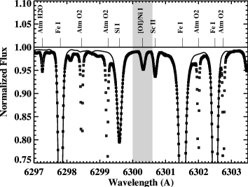
Figure 1: Solar spectrum in the vicinity of the [OI] line at 6300.312 Å. The points are from the NSO solar atlas, and the solid line is the SME fit. The shaded region marks the region that is included in the $\chi^{2}$ fit to the [OI]/NiI blend.

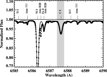
Figure 2: Solar spectrum in the vicinity of the CI line at 6587.625 Å. The points are from the NSO solar atlas, and the solid line is the SME fit. The shaded region marks the region that is included in the $\chi^{2}$ fit to the CI line.

Figure 3: The [OI]/NiI blend in the NSO spectrum. The points are the from NSO solar atlas, and the solid line is the SME fit. The relative contribution of [OI] and Ni are shown by the dashed and dotted lines respectively.

Figure 4: The CI line in the NSO spectrum. The points are the from NSO solar atlas, and the solid line is the SME fit. The fitting region for this line is 6587.4-6587.8 Å and excludes the unidentified feature at 6587.9.

Figure 5: Sample spectra of stars with low and high carbon and oxygen abundances. The solid line shows the best fit SME spectrum. The dashed lines are the SME spectra with [X/H] increased and decreased by 0.1 dex $\sim 25$% from the best fit value. The [OI] line in the HD 22879 spectrum sits between two telluric lines.

3.3 Telluric Rejection

There are several telluric lines from O₂ and H₂O in the vicinity of our indicators including the 6300.3 Å airglow (see Figures 1 and 2). These lines are produced in the rest frame of the Earth and contaminate different parts of a star’s spectrum depending on the relative line of sight velocity between the Earth and the star. We compute this velocity directly from the spectra, by cross-correlating the stellar spectra with the NSO solar atlas. Based on this velocity, we account for any shift in the location of the telluric line in the stellar rest frame.

If a telluric line enters the fitting region, we discard that observation. Figure 6 shows the [OI]/NiI blend from two different observations of HIP 92922: one where the blend is contaminated by a telluric absorption line and one where the blend is free from telluric contamination. We reject 53% of our [OI] spectra and 43% of our CI spectra because of telluric contamination. Telluric lines affect the [OI] region more strongly due to the airglow at 6300 Å.

Figure 6: Two spectra of HIP 92922 in the star’s rest frame. The [OI]/NiI region (marked with the solid line) in the upper panel is contaminated with an atmospheric O2 (marked with a dashed line). The same telluric absorption line is shifted 0.3 Å blueward in the lower panel and does not contaminate the [OI]/NiI blend.

3.4 Iodine Removal

The majority of the spectra in the CPS catalog were taken through the iodine cell. Iodine lines are $\sim 0.5$% deep in the CI region—comparable to the photon noise. In the [OI] region, they are a $\sim 5$% effect and must be removed. For a given iodine cell in observation, we locate the most recent iodine observation (usually at the beginning of the night). We account for any shift of the CCD between the two observations by cross-correlating spectral orders 8, 9, and 10 ($\lambda=$ 5608 - 5895Å, where the iodine lines are strongest). After removing any shift, we divide the iodine cell in observations by the iodine reference observations. Figure 7 shows a stellar spectrum, an iodine spectrum, and the ratio of the two.

Dividing the iodine spectrum from an iodine cell in spectrum cannot be done to within photon statistics. On nights of good seeing, a star’s image may be narrower than the HIRES slit. The reference iodine spectra are produced with a lamp that fills the slit uniformly, so the iodine lines from the iodine cell in observations can be narrower than the reference iodine lines. The result is artifacts from the division at the $\sim 1$% level. Iodine cell in spectra for a single star generally yield a larger spread in derived oxygen abundance compared to iodine cell out observations. However, when we plot oxygen abundances derived from iodine cell in observations against abundances from iodine cell out observations in Figure 8, we see no systematic trend.

Figure 7: HD 148284 spectrum with iodine contamination (top), reference iodine observation (middle), and stellar spectrum divided by iodine spectrum (bottom). The arrow marks the [OI]/NiI blend. The iodine is removed to a level of $\sim$1% of the continuum intensity.

Figure 8: Comparison of oxygen abundances derived from spectra taken with the iodine cell in (vertical axis) to those taken with the iodine cell out (horizontal axis). The solid line corresponds to an equality of the two, while the dashed line shows the best fit to the points. Apparently the oxygen abundances derived from both types of spectra show no systematic difference, indicating that the removal of the iodine spectrum works without introducing a systematic error.

3.5 Fitting Abundances

We converge on abundance by iterating three $\chi^{2}$ minimization routines that fit the continuum, line center, and abundance. Only points within the fitting range are used to calculate the $\chi^{2}$ statistic. Any point deviating from the fit by more than five times the photon noise is not included in calculating $\chi^{2}$. A short description of each routine is given below:

1. Continuum. Given the shallowness of our indicators, a small error in the continuum level will have a significant effect on the derived abundance. We refine the continuum value by registering the level of the spectrum so that $\chi^{2}$ is minimized.

2. Line center. The wavelength zero point and dispersion is initially determined from a thorium lamp calibration taken each night and refined by cross-correlating the observed spectrum with the solar spectrum. We adjust the radial velocity of the model spectrum to minimize $\chi^{2}$.

3. Abundance. We begin with the solar oxygen abundance scaled by the star’s metallicity. We refine this value by searching over 2 dex of abundance space and minimizing $\chi^{2}$.

We terminate the iteration when the fits arrive at a stable solution or when we exceed 10 iterations.

4 Results

4.1 Carbon and Oxygen Abundances

We report [O/H] and [C/H] for 694 and 704 stars respectively. These are subsamples of our initial 1070 star sample and arise after we apply the following global cuts:

1. $v\sin i$. In rapidly rotating stars, our indicators can be polluted by the wings of neighboring lines due to rotational broadening. When this happens, the abundances of our elements of interest become degenerate with that of the polluting line. This effect sets in earlier for the [OI] line, which sits shoulder to shoulder between SiI and ScII features. We do not report oxygen or carbon abundances for stars with $v\sin i$ greater than 7 and 15 km/s respectively.

2. $T_{eff}$. The high excitation energy of the CI line (8.537 eV) means the line is very weak in cool stars. For example, at 5000K, the line depth in a solar analog is 1%. We do not report carbon abundances for stars cooler than 5300 K.

3. Statistical scatter. We choose to report abundances for stars where the scatter in derived abundance is less than 0.30 dex or, in other words, stars where our measurements are precise to a factor of 2. Our estimates of measurement precision are based on empirical scatter and a Monte Carlo analysis, which we describe in sections § 4.2 & § 4.3. While our measurement precision is based on a variety of factors including line depth and signal to noise, stars that fail this cut generally have sub-solar carbon and oxygen abundances.

With our large stellar sample, it is possible to detect and correct for systematic trends that would be invisible in smaller samples. Figure 9 shows carbon and oxygen abundances plotted against temperature. We believe that the Kurucz (1992) model atmospheres are most accurate for solar analogs and that errors in the atmosphere profile grows as we move away from $T_{eff}=T_{\odot}$ =  5770 K.

We model the systematic behavior of implied abundance with $T_{eff}$ by fitting a cubic to the data. Simply subtracting out the cubic would artificially force the mean [X/H] to zero, but there is no reason why the mean disk abundance should be solar. Therefore, we let the solar abundance fix the constant term in the cubic by requiring the systematic correction be zero at 5770 K. This correction reaches 0.11 dex for oxygen and 0.15 dex for carbon. We have removed the temperature trend for all abundances quoted henceforth.

By removing abundance trends with $T_{eff}$ for the sake of correcting errors in atmosphere models, we may have erased a real astrophysical trend of [X/H] with $T_{eff}$. For example, hotter stars are more massive and have shorter main sequence lifetimes than cool stars. Therefore, the hotter stars in our sample are on average younger and formed at a later time in the galactic chemical enrichment history. However, we chose to remove the $T_{eff}$ trends because we believe uncertainties in atmospheric models are the dominant effect.

We report our temperature-corrected values for [O/H] and [C/H] with 85% and 15% confidence limits along with other stellar data in the Appendix. We summarize the statistical properties of derived abundances in Table 4.1 and show their distributions in Figure 10.

Table 3: Summary of Derived Abundances.

	N	m	S	Min	Max
		(dex)	(dex)	(dex)	(dex)
${[}O/H]$	694	0.06	0.14	-0.91	0.43
${[}C/H]$	704	0.09	0.17	-0.52	0.52
${[}Fe/H]$	1070	0.07	0.27	-1.95	0.56

Note. — Here, N is the number of stars with determined abundances, m is the mean abundance, and S is the standard deviation of abundance distribution.

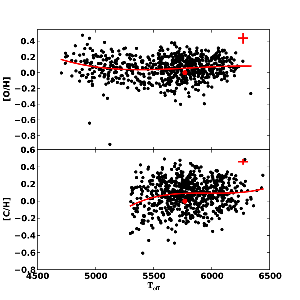
Figure 9: Plots showing systematic trends of [O/H] and [C/H] with temperature. The red line is the best fit cubic. Our correction for the $T_{eff}$trend is this cubic with the constant term chosen so that the correction is zero at $T_{eff}=$ 5770 K (large red dot). The crosses show the median errors.

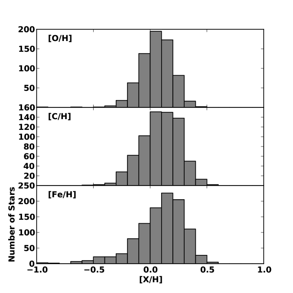
Figure 10: Distributions of [O/H], [C/H], and [Fe/H] for comparison.

4.2 Random Errors

We use Monte Carlo bootstrapping to estimate random errors. We generate Monte Carlo spectra by scrambling the residuals from our fits and adding them back to the synthetic spectra. For each star we generate and refit 1000 Monte Carlo realizations of the spectrum. The resulting abundance distribution provides a good estimate of the true error distribution.

For some stars we have many independent spectra, allowing us to compute confidence limits of the oxygen abundances from them as an empirical measure of our internal errors. Figure 11 shows the length of the error bars computed empirically and from Monte Carlo for stars with more than 50 empirical fits. The error estimate from Monte Carlo tracks the empirical scatter well, slightly overestimating it. This is due to systematic errors in our fits that appear as random errors when we scramble the residuals.

For stars with fewer than 20 observations, we adopt the Monte Carlo confidence intervals as our statistical error; for stars with 20 or more observations, we adopt the empirical confidence intervals. We diminish these errors by $\sqrt{N_{obs}}$. Futhuremore, we impose an error floor of 0.03 dex.

Figure 11: Scatter in MC simulations as a function of empirical scatter for stars with more than 50 observations. Oxygen and carbon measurements are represented by circles and triangles respectively. The solid line represents a 1:1 correlation.

4.3 Nickel Systematics

Since we are deriving oxygen from a line that is blended with nickel, the errors in nickel abundance are covariant with errors in oxygen abundance. FV05 quote a uniform error of 0.03 dex for their nickel measurements. The amount that [OI] and NiI contribute to the blend is different for every star. Therefore, we evaluate the effect of the 0.03 dex error in nickel abundance on oxygen abundance on a star-by-star basis. We begin with a synthetic spectrum at our quoted oxygen abundance. We then refit the oxygen line to a spectrum with 0.03 dex more and 0.03 dex less nickel. These errors are added in quadrature to the statistical errors.

There are many other sources of systematic error in our abundance measurements such as inaccurate solar reference abundances, additional blends, and our assumption of LTE. However, these effects should be largely consistent between stars, so we expect them to contribute little to errors in our differential abundances.

4.4 Comparison with Literature

We compare our results with Bensby et al. (2005) and Luck & Heiter (2006). We report oxygen abundances for 16 stars analyzed by Bensby et al. (2005) and 67 stars analyzed by Luck & Heiter (2006). We plot the comparison in Figure 12. Our results track these comparison studies well. We recognize that the agreement is poorest for low values of [C/H]. This likely the result of less robust fits to stars with weaker carbon features.

The standard deviation of the differences in derived abundances is 0.08 dex for oxygen and 0.09 dex for carbon. Since Bensby et al. (2005) and Luck & Heiter (2006) use different instruments, spectral synthesizers, and fitting algorithms, it is unlikely there are common systematic errors. Therefore, the scatter in the differences can be interpreted as a measure of the typical combined statistical and systematic error. We cannot say how much of the observed scatter is due to our errors and those of the comparison studies.

Figure 12: Comparison plots of abundances from this work against those of Bensby et al. (2005) and Luck & Heiter (2006). The line shows a 1:1 correlation. We note a systematic offset in the carbon comparison. This may stem from the fact that the two works use different indicators.

4.5 Abundance Trends in the Thin and Thick Disks

The Milky Way is thought to be made up of three distinct star populations: The thin disk, thick disk, and the halo. Most of the stars in the local neighborhood belong to the thin disk, which has a scale height of 300 pc. The thick disk has a scale height of 1450 pc and is comprised of older, metal-poor stars.

Peek (2009) combined proper motion measurements from the Hipparcos catalog (ESA 1997) with radial velocity measurements from the Nidever et al. (2002), SPOCS, and N2K catalogs into three-dimensional space motions for 1025 of our 1070 program stars. Peek (2009) computed the probability of membership to each of the three populations in the manner of Bensby et al. (2003), Mishenina et al. (2004), and Reddy et al. (2006) for 900 of our 941 stars with measured carbon and oxygen. Our sample contains 847 thin disk stars, 16 thick disk stars, 12 halo stars, and 25 borderline stars (all three membership probabilities less than 0.7).

We plot [O/H] and [C/H] against [Fe/H] in Figure 13. We fit the trends with a line and list the best fit parameters in Table 4.5. If the scatter was purely statistical, we would expect our fits to have a reduced-$\sqrt{\chi^{2}}\sim 1$. Our fits have reduced-$\sqrt{\chi^{2}}\sim 2$, which suggests that some of the observed scatter is astrophysical. These main sequence stars have not begun to process heavy elements, so the ranges of C, O, and Fe ratios reflect the heterogeneous interstellar medium from which they formed.

Table 4: Best fit parameters to abundance trends.

Note. — We fit thin and thick disk abundance trends with the following function [X/H] = $m$ [X/Fe] + $b$. The best fit parameters are listed above along with the reduced-$\sqrt{\chi^{2}}$.

We also plot [O/Fe] and [C/Fe] against [Fe/H] in Figure 14. The trends suggest that carbon and oxygen lagged behind iron production for much of the period of galactic chemical enrichment. These trends flatten out for high [Fe/H]. Due to the paucity of thick disk stars in our sample, we are cautious in interpreting its abundance trends. However, in the thick disk, oxygen seems to be enhanced relative to iron, a result also reported by Bensby et al. (2004). This enhancement in oxygen suggests that type II supernova played a more active role in enriching the thick disk.

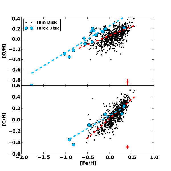
Figure 13: Carbon and oxygen abundance plotted against iron abundance. The black points are the thin disk stars; the blue points are the thin disk stars. The line shows the abundance ratios in 0.1 dex bins. The crosses show median uncertainties.

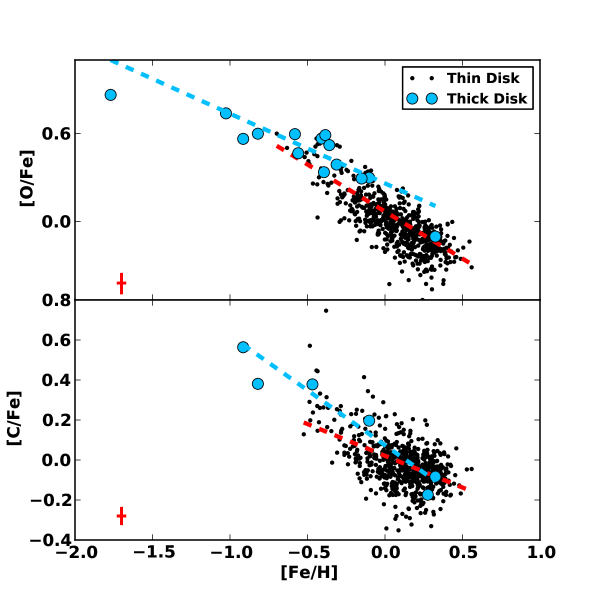
Figure 14: The ratios of carbon and oxygen to iron plotted against iron abundance. The black points are the thin disk stars; the blue points are the thin disk stars. The line shows the average ratios in 0.1 dex bins. The crosses show median uncertainties.

4.6 Exoplanets

100 stars in our initial 1070 sample are known to host planets. Gonzalez (1997) measured relatively high stellar metallically in the first four exoplanet host stars, and Santos et al. (2004) and Fischer & Valenti (2005) showed that the fraction of stars bearing planets increases rapidly above solar metallicity. In light of the correlation between C, O, and Fe, it is not surprising that hosts to exoplanets are enriched in carbon and oxygen relative to the comparison sample.

As shown in Table 4.6, the mean [O/H] of the planet host and comparison sample is 0.10 dex and 0.05 dex respectively. If we take the error on the mean abundance to be the standard deviation of derived abundances divided by the square root of the number of stars in each sample i.e. $\sigma_{mean}=\frac{\mathrm{Std.\ Dev.}}{\sqrt{N}}$, $\sigma_{mean}$ for [O/H] is 0.01 dex. Carbon is also enriched in planet hosts where the mean [C/H] is 0.17 dex ($\sigma_{mean}=0.02$ dex) compared to 0.08 dex in the comparison sample with. For both carbon and oxygen, the mean abundance of the planet host sample is enriched by $\sim 5\sigma$ compared to the non-host sample.

In Figure 15, we divide the stars into 0.1 dex bins in [X/H]. For each bin, we divide the number of planet-bearing stars by the total number of stars in the bin. As with iron, we observe an increase in planet occurrence rate as carbon and oxygen abundance increases. While there is a hint of a possible plateau or turnover at the highest abundance bins, these bins are dominated by small number statistics. The data are not inconsistent with a monotonic rise, within the errors. The possibility that very enriched systems inhibit planet formation is intriguing, and this parameter space warrants further exploration.

Table 5: Statistical abundance properties of stars with planets.

Note. — We list the number of stars, mean abundance (dex), standard deviation (dex), and error on the mean abundance (dex) for the host and non-host populations. The error on the mean abundance is computed by $\sigma_{mean}=\frac{\mathrm{Std.\ Dev.}}{\sqrt{N}}$.

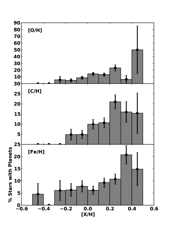
Figure 15: The percentage of stars with known planets for 0.1 dex bins in oxygen, carbon, and iron. The histograms are constructed from the 694, 704, and 1070 stars with reliable measurements of [O/H], [C/H], and [Fe/H] respectively.

4.7 $N_{C}/N_{O}$

We present the ratio of carbon to oxygen atoms, $N_{C}/N_{O}$ for 457 stars with reliable carbon and oxygen measurements as listed in the last column of Table 5 of the Appendix. Since we do not report carbon for stars cooler than 5300 K, our $N_{C}/N_{O}$ measurements apply only to F and G spectral types. While there is a weak correlation between $N_{C}/N_{O}$ and Fe at high [Fe/H], we note the large degree of scatter in $N_{C}/N_{O}$, which spans a wide range from 0.24 to 1.55.

We emphasize that our measurements of [C/H] and [O/H] are differential relative to solar and should be insensitive to revisions in the solar abundance distribution. $N_{C}/N_{O}$ depends on our adopted solar abundances of of oxygen (Scott et al. 2009) and carbon (Caffau et al. 2010). We believe the abundances of carbon and oxygen are known at the $\sim 0.1$ dex level. Therefore, we expect revisions to the solar abundance distribution to systematically shift our $N_{C}/N_{O}$ measurements by roughly $\sim 10^{0.1}$ or $\sim 25\%$

We measure 46 stars with $N_{C}/N_{O}$ greater than 1.00. Given the size of our random errors as determined by the Monte Carlo analysis of § 4.2, very few of these stars are $1\sigma$ detections of $N_{C}/N_{O}>1.$ However, since these errors are random, we believe our measurements accurately reflect the distribution of $N_{C}/N_{O}$ in nearby disk stars. Neglecting the zero-point offsets discussed earlier, we measure $N_{C}/N_{O}>1$ for roughly 10% of nearby FG stars.

As noted by our anonymous reviewer, the CO molecule controls the equilibrium between carbon and oxygen in M dwarfs. It is believed that $N_{C}/N_{O}>1$ in M dwarfs results in an atmosphere rich in C₂, while $N_{C}/N_{O}<1$ gives rise to TiO. We are unaware of M dwarfs with strong C₂ bands indicating $N_{C}/N_{O}>1$. This suggests such a population is rare, assuming we understand the behavior of carbon-rich M dwarf atmospheres. We also note the additional complexities involved in modeling M star atmospheres. Abundance estimates in cool stars rely on opacity tables of H₂O and other molecules that are not well understood at the temperatures probed by M star atmospheres. The fact that M stars are fully convective and have strong magnetic fields introduce additional complexities into model atmospheres.

Despite the uncertainties in accurately measuring $N_{C}/N_{O}$, we have characterized the distribution of $N_{C}/N_{O}$ for an unprecedented number of FG stars. Furthermore, we have identified 46 stars have high $N_{C}/N_{O}$. Given the predictions regarding exotic planets that form in a carbon rich environment, these stars constitute important hosts for future work on their exoplanets and exozodiacal dust. Observations of dust with ALMA and JWST may be particularly valuable.

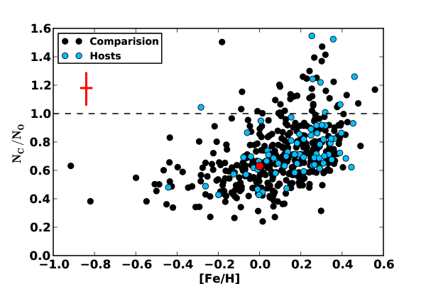
Figure 16: $N_{C}/N_{O}$ as a function of iron abundance. The large red dot shows the solar values. The horizontal line shows equal carbon and oxygen.

4.8 WASP-12

WASP-12b, discovered by Hebb et al. (2009), is a transiting gas giant and a favorable target for atmosphere studies. Campo et al. (2011) and Croll et al. (2011) measured secondary eclipses of WASP-12b at wavelengths ranging from 1-8 $\mu$m, which can be used to characterize the planet’s dayside emission spectrum. In a recent study, Madhusudhan et al. (2011) found that these measurements are best-described by atmosphere models with $N_{C}/N_{O}$ $\geq$ 1 at 3 sigma significance.

We analyze WASP-12 identically to the 1070 star sample. With a V-mag of 11.69 (Hebb et al. 2009), WASP-12 is dimmest star in this work and our spectra have S/N $\sim$ 50. However, we measured oxygen and carbon based on 9 and 7 spectra respectively. We find [O/H] = $0.29_{-0.10}^{+0.06}$, [C/H] = $0.10_{-0.06}^{+0.04}$, and $N_{C}/N_{O}$ = $0.40_{-0.07}^{+0.11}$ i.e., sub-solar.

If the composition of the host star truly reflects the material from which WASP-12b formed, our measurements suggest that WASP-12b does not have a carbon-dominated bulk composition. It is possible that the planet acquired extra carbon at some point during its formation, or that the planet’s nightside and/or interior are acting as a sink for oxygen, creating a carbon-rich dayside atmosphere while maintaing bulk $N_{C}/N_{O}$ less than unity. In any case, this planet and its host star warrant further study.

5 Conclusion

We have presented oxygen and carbon abundances for 941 stars based on HIRES spectra gathered by the Keck telescope. We measure oxygen by fitting the reliable 6300 Å forbidden line with SME and self-consistently account for the significant nickel blend. Our carbon abundances are derived from the 6587 Å  CI line. Our errors are based on a rigorous Monte Carlo treatment, and our measurements agree with values in the literature. Our sample is large enough to characterize and remove systematic trends due to $T_{eff}$. We see that carbon and oxygen are both enriched in stars with known planets. We see a significant number of stars with $N_{C}/N_{O}$ exceeding unity, which supports the possibility that some stars host exotic carbon-rich planets. However, our measurement of sub-solar $N_{C}/N_{O}$ for WASP-12, complicates the recent claim by Madhusudhan et al. (2011) that WASP-12b is a carbon world.

Table 6: Stellar Data.

References

- Allende Prieto et al. (2001) Allende Prieto, C., Lambert, D. L., & Asplund, M. 2001, ApJ, 556, L63
- Bensby et al. (2003) Bensby, T., Feltzing, S., & Lundström, I. 2003, A&A, 410, 527
- Bensby et al. (2004) —. 2004, A&A, 415, 155
- Bensby et al. (2005) Bensby, T., Feltzing, S., Lundström, I., & Ilyin, I. 2005, A&A, 433, 185
- Bond et al. (2010) Bond, J. C., Lauretta, D. S., & O’Brien, D. P. 2010, in IAU Symposium, Vol. 265, IAU Symposium, ed. K. Cunha, M. Spite, & B. Barbuy, 399–402
- Caffau et al. (2010) Caffau, E., Ludwig, H., Bonifacio, P., Faraggiana, R., Steffen, M., Freytag, B., Kamp, I., & Ayres, T. R. 2010, A&A, 514, A92+
- Campo et al. (2011) Campo, C. J., et al. 2011, ApJ, 727, 125
- Croll et al. (2011) Croll, B., Lafreniere, D., Albert, L., Jayawardhana, R., Fortney, J. J., & Murray, N. 2011, AJ, 141, 30
- Edvardsson et al. (1993) Edvardsson, B., Andersen, J., Gustafsson, B., Lambert, D. L., Nissen, P. E., & Tomkin, J. 1993, A&A, 275, 101
- ESA (1997) ESA. 1997, VizieR Online Data Catalog, 1239, 0
- Fischer & Valenti (2005) Fischer, D. A., & Valenti, J. 2005, ApJ, 622, 1102
- Fischer et al. (2005) Fischer, D. A., et al. 2005, ApJ, 620, 481
- Gonzalez (1997) Gonzalez, G. 1997, MNRAS, 285, 403
- Grevesse & Sauval (1998) Grevesse, N., & Sauval, A. J. 1998, Space Science Reviews, 85, 161
- Gustafsson et al. (1999) Gustafsson, B., Karlsson, T., Olsson, E., Edvardsson, B., & Ryde, N. 1999, A&A, 342, 426
- Hebb et al. (2009) Hebb, L., et al. 2009, ApJ, 693, 1920
- Johansson et al. (2003) Johansson, S., Litzén, U., Lundberg, H., & Zhang, Z. 2003, ApJ, 584, L107
- Kuchner & Seager (2005) Kuchner, M. J., & Seager, S. 2005, ArXiv Astrophysics e-prints
- Kurucz (1992) Kurucz, R. L. 1992, in IAU Symposium, Vol. 149, The Stellar Populations of Galaxies, ed. B. Barbuy & A. Renzini, 225–+
- Kurucz et al. (1984) Kurucz, R. L., Furenlid, I., Brault, J., & Testerman, L. 1984, Solar flux atlas from 296 to 1300 nm, ed. Kurucz, R. L., Furenlid, I., Brault, J., & Testerman, L.
- Lambert (1978) Lambert, D. L. 1978, MNRAS, 182, 249
- Luck & Heiter (2006) Luck, R. E., & Heiter, U. 2006, AJ, 131, 3069
- Madhusudhan et al. (2011) Madhusudhan, N., et al. 2011, Nature, 469, 64
- Marcy & Butler (1992) Marcy, G. W., & Butler, R. P. 1992, PASP, 104, 270
- Marcy et al. (2008) Marcy, G. W., et al. 2008, Exoplanet properties from Lick, Keck and AAT
- Mishenina et al. (2004) Mishenina, T. V., Soubiran, C., Kovtyukh, V. V., & Korotin, S. A. 2004, A&A, 418, 551
- Nidever et al. (2002) Nidever, D. L., Marcy, G. W., Butler, R. P., Fischer, D. A., & Vogt, S. S. 2002, ApJS, 141, 503
- Nordström et al. (2004) Nordström, B., et al. 2004, The Messenger, 118, 61
- Peek (2009) Peek, K. 2009, PhD thesis, University of California, Berkeley
- Piskunov et al. (1995) Piskunov, N. E., Kupka, F., Ryabchikova, T. A., Weiss, W. W., & Jeffery, C. S. 1995, A&AS, 112, 525
- Ramírez et al. (2007) Ramírez, I., Allende Prieto, C., & Lambert, D. L. 2007, A&A, 465, 271
- Reddy et al. (2006) Reddy, B. E., Lambert, D. L., & Allende Prieto, C. 2006, MNRAS, 367, 1329
- Santos et al. (2004) Santos, N. C., Israelian, G., & Mayor, M. 2004, A&A, 415, 1153
- Scott et al. (2009) Scott, P., Asplund, M., Grevesse, N., & Sauval, A. J. 2009, ApJ, 691, L119
- Valenti & Fischer (2005) Valenti, J. A., & Fischer, D. A. 2005, ApJS, 159, 141, (VF05)
- Valenti & Piskunov (1996) Valenti, J. A., & Piskunov, N. 1996, A&AS, 118, 595
- Vogt et al. (1994) Vogt, S. S., et al. 1994, in Society of Photo-Optical Instrumentation Engineers (SPIE) Conference Series, Vol. 2198, Society of Photo-Optical Instrumentation Engineers (SPIE) Conference Series, ed. D. L. Crawford & E. R. Craine, 362–+