The role of environmental correlations in the non-Markovian dynamics of a spin system

Abstract

We put forward a framework to study the dynamics of a chain of interacting quantum particles affected by individual or collective multi-mode environment, focussing on the role played by the environmental quantum correlations over the evolution of the chain. The presence of entanglement in the state of the environmental system magnifies the non-Markovian nature of the chain’s dynamics, giving rise to structures in figures of merit such as entanglement and purity that are not observed under a separable multi-mode environment. Our analysis can be relevant to problems tackling the open-system dynamics of biological complexes of strong current interest.

The investigation on the interaction between a spin-like two-level system (TLS) and an environment embodied by an ensemble of harmonic oscillators, the so-called spin-boson model LeggettReview , has gained renewed momentum due to the current strong interest in the quantum-mechanical description of excitation-transfer processes in biological organisms or the dynamics of protein-solvent systems in photosynthetic complexes  Huelga ; Reina ; lloyd ; scholak ; Huelga2 . The interest in such a celebrated model is twofold, in this context. On one side, it is employed to understand the active role of an environment in assisting transport across such structures lloyd . On the other hand, the model is extremely useful to characterize the extent to which non-classical behaviors survive in systems affected by environmental worlds that are strictly adherent to the paradigm of being wet and warm. In this respect, we aim at gathering a description of the TLS-environment evolution that is as complete as possible and able to account for subtle yet potentially key features of such dynamics emerging from the finiteness the environment itself, its capability to retain information on the system it is coupled to (and kick it back at later times) and its inherent structure. For, instance, Rebentrost et al. have shown in Ref. nmqj that environmental memory-keeping effects are crucial for preserving the coherent behavior of excitonic energy transfer processes in biological complexes.

Stepping aside from interesting yet still controversial bio-physical scenarios, the general model addressed above plays an important role in various contexts of applied quantum physics, from cavity quantum electrodynamics to its solid-state analogues involving defects in diamond coupled to semiconducting microcavities diamond or superconducting devices and planar strip-line resonators cqed . In the latter case, very interesting regimes are quickly becoming available where the coupling strength of the coherent part of an evolution can be made comparable to the one responsible for the open-system dynamics due to the presence of the environment bourassa .

All such considerations and physical configurations demand the development of a framework apt to encompass and harness features of non-Markovianity in various coupling regimes. Formally, one is required to retain, to some extent, the degrees of freedom of the environment so as to allow for its possibly-non-trivial structure to influence the dynamics of the system of interest. This can be computationally very demanding and while sophisticated techniques have been put forward to determine the quantum statistical properties of interacting quantum many-body systems, they are either hardly suitable for non-linear configurations or face some difficulties in tracking the temporal dynamics of the system itself.

In this paper we contribute to the investigation on the interaction between a system of interacting TLS’s coupled to a bosonic environment by studying the effect that environmental entanglement has on the dynamics of a chain of interacting TLS’s. We build up a mathematical apparatus that, inspired by and significantly extending the approach in Ref. massimo , solves exactly the local interaction between a single TLS and its multi-mode environment, so as to build an eigenbasis that is then used in order to tackle the inter-particle coupling by keeping track of the environmental properties. This helps us in incorporating the full quantum features of the environmental state, therefore enabling a quantitative study of the role of entanglement in the evolution of the chain under investigation and its relation to the non-Markovian nature of the dynamics. We illustrate our techniques by addressing the cases of a dimer and a trimer, which are the smallest non-trivial configurations allowing us to study the most crucial attributes of such a complex problem. Our investigation opens up the possibility to study full-scale networks of coupled TLS’s in an open-system fashion, covering the full range of coupling strengths with the environments, from the weak to the strong one. Although inevitably leaving a few questions open, we believe such an endeavor to be helpful in the contexts described above.

The remainder of this paper is organized as follows: in Sec. I we describe the method put forward in order to analyze the dynamics of an $N$-site chain interacting with individual multi-mode bosonic environments without resorting to the weak-coupling regime and thus allowing for a more complete overview of the effects of non-Markovianity on the evolution of the chain. Sec. II is devoted to the explicit study on a dimer of interacting particles affected by entangled environments. The key features in the dynamics of such configuration are compared to what is achieved under the assumption of independent environments so as to show that entanglement appear to enhance the non-Markovian aspects of the time evolution. Sec. III addresses the case of a common environment affecting the sites of our dimer, showing that the manifestations mentioned above are insensitive to the non-local nature of the environment, but rather depend on the properties of its state such as the entanglement-sharing structure, as studied in Sec. IV for the case of a trimer. Finally, in Sec. V we draw our conclusions and briefly discuss the questions opened by our investigation.

I The model and the analytical method to its approach

The model under consideration is described by an Hamiltonian of the form

$$\mathbf{\hat{H}_{tot}=\hat{H}_{S}+\hat{H}_{SS}+\hat{H}_{B}+\hat{S}_{SB}}.$$ (1)

Here $\mathbf{\hat{H}_{S}}=-\hbar\sum_{j=1}^{N}\epsilon_{j}\hat{\sigma}_{j}^{z}$ gives the free dynamics of the elements of the chain, $\epsilon_{j}$ being the energy split between the levels of each TLS, while $\{\hat{\sigma}_{j}^{x},\hat{\sigma}_{j}^{y},\hat{\sigma}_{j}^{z}\}$ are the Pauli matrices for particle $j{=}1,..,N$. Analogously, $\mathbf{\hat{H}_{B}}{=}\sum_{j=1}^{N}\sum^{n_{j}}_{k=1}{\hbar\omega_{j,k}\hat{a}_{j,k}^{{\dagger}}\hat{a}_{j,k}}$ is the free energy of the environmental harmonic oscillators. The pedex $k$ labels the $n_{j}$ independent modes interacting with the TLS at site $j$. Each of such modes has frequency $\omega_{j,k}$ and is described by the bosonic annihilation [creation] operator $\hat{a}_{j,k}$ [$\hat{a}_{j,k}^{\dagger}$]. On the other hand, $\mathbf{\hat{H}_{SS}}$ models the inter-particle coupling within the chain, while $\mathbf{\hat{H}_{SB}}$ describes the TLS-environment interaction. We take these two terms as

$$\mathbf{\hat{H}_{SB}}= \sum_{j=1}^{N}\hat{\sigma}_{j}^{z}\otimes\sum^{n_{j}}_{k=1}g_{j,k}(\hat{a}_{j,k}^{\dagger}+\hat{a}_{j,k}),$$ (2)

$$\mathbf{\hat{H}_{SS}}= -2\hbar\sum_{n=j}^{N-1}J_{j,j+1}(\hat{\sigma}_{j}^{x}\hat{\sigma}_{j+1}^{x}+\hat{\sigma}_{j}^{y}\hat{\sigma}_{j+1}^{y})$$

with $J_{j,j+1}$ being the nearest-neighbor coupling strength between the particles occupying sites $j$ and $j+1$ on the chain and $g_{j,k}$ the analogous parameter associated with the interaction of the $j^{\text{th}}$ TLS and its $k^{\text{th}}$ environmental mode.

The first of Eq. (2) generates a displacement of the environmental oscillators, conditioned on the state of the corresponding TLS. Our approach to the description of the dynamics is to solve the problems embodied by each the subsystem made out of a single TLS and the ensemble of local modes it interacts with. We thus consider $\mathbf{\hat{H}}_{\mathbf{0}}^{j}=\mathbf{\hat{H}}_{\mathbf{S}}^{j}+\mathbf{\hat{H}}_{\mathbf{B}}^{j}+\mathbf{\hat{H}}_{\mathbf{SB}}^{j}$ and look for eigenstates of the form $|a\rangle_{j}\otimes|\phi_{i}\rangle_{j}$ with $a=\pm$ and $\{\left|\pm\right\rangle_{j}\}$ denoting the eigenbasis of $\hat{\sigma}^{z}_{j}$. States $|\phi_{i}\rangle_{j}$ are the eigenstates of the total Hamiltonian of an ensemble of oscillators (per assigned state of the corresponding TLS), that is

$$\sum^{n_{j}}_{k=1}[\pm g_{j,k}(a_{j,k}^{{\dagger}}{+}a_{j,k})+\hbar\omega\hat{a}_{j,k}^{{\dagger}}\hat{a}_{j,k}]\!|\phi_{\pm}\rangle_{j}{=}(E^{j}\pm\epsilon_{j})|\phi_{\pm}\rangle_{j},$$ (3)

where $E^{j}$ is the total energy of the $j^{\text{th}}$ subsystem. A detailed calculation shows that such energy depends on the number of excitations $n_{j,k}$ in the oscillators coupled to the TLS at the $j^{\text{th}}$ site according to the expression

$$E^{j}_{n}=\pm\epsilon_{j}+\sum^{n_{j}}_{k=1}\hbar\omega_{j,k}(n_{j,k}-{\alpha_{j,k}^{2}}),$$ (4)

where $\alpha_{j,k}=g_{j,k}/\hbar\omega_{j,k}$. The corresponding eigenstates can be written as $|\psi_{\pm}^{{\bf n}_{j}}\rangle_{j}{=}|\pm\rangle_{j}{\otimes}|\alpha_{\pm}^{{\bf n}_{j}}\rangle_{j}{=}|\pm\rangle_{j}{\otimes^{n_{j}}_{k=1}}|\alpha_{\pm}^{n_{k}}\rangle_{j}$, where ${\bf n}_{j}=\{n_{1},n_{2},..,n_{n_{j}}\}$ is the vector specified by the number of excitations populating the $n_{j}$ oscillators interacting with the $j^{\text{th}}$ TLS and we have introduced the excitation-added coherent states $|\alpha_{\pm}^{n_{k}}\rangle{=}[{(a^{{\dagger}}_{j}\pm\alpha_{j,k})^{n_{k}}}/{\sqrt{n_{k}!}}]|\pm\alpha_{j,k}\rangle$. Although it is straightforward to check that $\langle\alpha_{+}^{m}|\alpha_{+}^{n}\rangle{=}\delta_{mn}$ ($\langle\alpha_{-}^{m}|\alpha_{-}^{n}\rangle{=}\delta_{mn}$) and the set of states $\{|+,\alpha_{+}^{n}\rangle\}$ ($\{|-,\alpha_{-}^{n}\rangle\}$) form an orthonormal basis, states $|\alpha_{+}^{n}\rangle$ and $|\alpha_{-}^{n}\rangle$ are not mutually orthogonal. A treatment with an arbitrary number of modes per site, performed along the lines of the discussion above, is certainly possible although computationally demanding. Therefore, from now on, we will focus our attention to the case of a single mode per site and drop the mode-label.
In the oscillator basis discussed above, the Hamiltonian (1) takes the form

$$\mathbf{\hat{H}_{tot}}=\sum_{j=1}^{N}\mathbf{\hat{H}}_{\mathbf{0}}^{j}+\mathbf{\hat{H}_{SS}},$$ (5)

each $\mathbf{\hat{H}}_{\mathbf{0}}^{j}$ being now diagonal. The remaining term $\mathbf{\hat{H}_{SS}}$, which is defined in the second line of Eq. (2), only contains the degrees of freedom of the TLS chain. In the following, we consider a homogeneous chain with $J_{j,j+1}=J,~{}\forall{j}=1,..,N$. By introducing the raising and lowering operators $\hat{\sigma}^{\pm}_{j}=(\hat{\sigma}^{x}_{j}\pm i\hat{\sigma}^{y}_{j})/2$, it is convenient to rewrite it as

$$\mathbf{\hat{H}_{SS}}=-\hbar J\sum_{n=1}^{N-1}(\hat{\sigma}_{j}^{+}\hat{\sigma}_{j+1}^{-}+\hat{\sigma}_{j}^{-}\hat{\sigma}_{j+1}^{+}).$$ (6)

In the interaction picture defined with respect to the unperturbed Hamiltonian $\mathbf{\hat{H}_{0}}{=}\sum_{j}\mathbf{\hat{H}}_{\mathbf{0}}^{j}$, we get

$$\mathbf{\hat{H}_{I}}(t){=}-\hbar J\!\!\left(\prod_{j=1}^{N}\hat{\Theta}^{\pm}_{j}\right)\!\sum_{n=1}^{N-1}(\sigma_{n}^{+}\sigma_{n+1}^{-}+h.c.)\!\left(\prod_{k=1}^{N}\hat{\Theta}^{\pm}_{k}\right)^{{\dagger}}$$ (7)

with $\hat{\Theta}^{\pm}_{j}=\sum_{n=0}^{\infty}{e^{iE_{\pm}^{n}t}|\pm,\alpha_{\pm}^{n}\rangle\langle\pm,\alpha_{\pm}^{n}|}$.
After elaborating on this expression, we obtain

$$\mathbf{\hat{H}_{I}}(t)=-\hbar J\sum_{n=1}^{N-1}(\hat{\sigma}_{n}^{+}\hat{\sigma}_{n+1}^{-}\hat{\Theta}^{+}_{n}\hat{\Theta}^{-}_{n+1}\hat{\Theta}^{-{\dagger}}_{n}\hat{\Theta}^{+{\dagger}}_{n+1}+h.c.).$$ (8)

By expanding the $\hat{\Theta}^{\pm}_{n}$’s in a coherent-state basis, we finally arrive at the effective expression for the intra-chain Hamiltonian

$$\mathbf{\hat{H}_{I}}(t)=-\hbar J\sum_{n=1}^{N-1}[\hat{\Gamma}_{n}^{+}\hat{\Gamma}_{n+1}^{-}+\hat{\Gamma}_{n}^{-}\hat{\Gamma}_{n+1}^{+}],$$ (9)

where $\hat{\Gamma}^{\pm}_{j}=\hat{\sigma}^{\pm}_{j}\otimes\hat{D}_{j}[\pm\alpha(t))]$ with $\hat{D}(\xi)$ the displacement operator of amplitude $\xi\in\mathbb{C}$ barnettradmore and $\alpha_{j}(t)=2\alpha_{j}(1-e^{i\omega_{j}t})$. While the analysis above explicitly consider individual environments affecting the elements of the chain, one can also study the complementary situation where all the TLS’s collectively interact with a single (and common) ensemble of oscillators. In this case, $[\mathbf{\hat{H}_{tot}},\sum_{j}\hat{\sigma}_{z}^{j}]{=}0$, which in turn implies that $\mathbf{H_{SS}}$ can be easily diagonalized. We tackle an explicit example of this situation in Sec. III.

In order to obtain information on the full dynamics of the TLS subsystem, we write the density matrix $\rho(t)$ of the chain-oscillators system in the excitation-added displaced basis. For all our simulations, we assume the factorized initial state

$$\rho(0)=\rho_{\text{chain}}(0)\otimes\rho_{\text{ho}}(0)$$ (10)

with $\rho_{\text{chain}}(t)$ [$\rho_{\text{ho}}(t)$] describing the state of the chain (oscillator environment) at time $t$. In what follows we consider two significant instances of $\rho_{\text{ho}}(0)$: the tensor product of individual thermal states and the case of entangled oscillators prepared in $N$-mode squeezed states barnettradmore . As it will be discussed later on, such three paradigmatic cases allow us to well identify the effect of the entanglement among the environments on the dynamics of the TLS’s.

Let us start addressing the case of a thermal state

$$\rho_{\text{th}}=\underset{j=1}{\overset{N}{\bigotimes}}\sum_{l=0}^{\infty}\dfrac{\overline{n}^{l}_{j}}{(1+\overline{n}_{j})^{l+1}}|l\rangle_{j}\langle l|,$$ (11)

where $\overline{n}_{j}{=}(e^{\beta\hbar\omega_{j}}{-}1)^{-1}$ is the average number of quanta in the oscillator at temperature $T$ (we have taken the inverse temperature $\beta=1/k_{b}T$ with $k_{b}$ the Boltzmann constant) and $\left|l\right\rangle$ is the state with $l$ excitations. In the excitation-added displaced basis of the oscillators, we can recast $\rho_{\text{th}}$ into the form

$$\rho_{\text{th}}{=}\underset{j=1}{\overset{N}{\bigotimes}}\sum_{n,m,l=0}^{\infty}\dfrac{\overline{n}^{l}_{j}}{(1+\overline{n}_{j})^{l+1}}|\alpha_{\pm}^{n}\rangle_{j}\langle\alpha_{\pm}^{n}|l\rangle_{j}\langle l|\alpha_{\pm}^{m}\rangle_{j}\langle\alpha_{\pm}^{m}|,$$ (12)

where the $+$ or $-$ sign for the $j^{\text{th}}$ oscillator has to be chosen according to the state of the corresponding element in $\rho_{\text{chain}}$. The scalar products $\langle\alpha_{\pm}^{n}|l\rangle$ needed for the evaluation of the expression above are given in terms of Charlier polynomials $C_{n}(m;\alpha^{2})$ as AS ; comment

$$\langle\alpha_{-}^{n}|m\rangle =\dfrac{\alpha^{n+m}e^{-\alpha^{2}/2}}{\sqrt{n!}\sqrt{m!}}C_{n}(m;\alpha^{2}),$$ (13)

$$\langle\alpha_{+}^{n}|m\rangle =\dfrac{\alpha^{n+m}e^{-\alpha^{2}/2}}{\sqrt{n!}\sqrt{m!}}C_{m}(n;\alpha^{2}),$$

where we have assumed $\alpha\in\mathbb{R}$. In the remainder of the manuscript we take $\overline{n}_{j}=\overline{n},\,\,\forall{j}$. We will also consider an $N$-mode a pure squeezed-vacuum state for the harmonic oscillators $\left|\text{sq}_{N}\right\rangle{=}(1{-}\lambda^{2})^{-1/2}\sum_{l}\lambda^{l}\otimes^{N}_{j=1}\left|l\right\rangle_{j}$ with $\lambda=\tanh r$ and $r$ the squeezing parameter. This state can be expressed in the chosen oscillator basis following the very same lines highlighted above and using again the Charlier polynomials. It is worth emphasizing that these two environmental states are locally indistinguishable as a squeezed vacuum is locally equivalent to a thermal state.

II Chain dynamics under independent environments

We are now in a position to start addressing the effective dynamics of the TLS chain under the influences of the various instances of environment introduced in the previous Section. In order to strip down our discussion from unnecessary complications, we study here the smallest configuration of the model at hand, i.e. a two-TLS chain (a dimer) affected by two individual harmonic oscillators, one per site. The two TLS will be considered as identical. While embodying an interesting enough situation Reina , this case allows for an agile description of the physics involved.

In the dimer basis, the interaction hamiltonian in Eq. (9) takes the form

$$\mathbf{\hat{H}_{I}}(t)=\left(\begin{array}[]{cccc}0&0&0&0\\ 0&0&\hat{D}_{1}(\alpha_{1})\hat{D}^{\dagger}_{2}(\alpha_{2})&0\\ 0&\hat{D}^{\dagger}_{1}(\alpha_{1})\hat{D}_{2}(\alpha_{2})&0&0\\ 0&0&0&0\\ \end{array}\right)$$ (14)

In order to simplify the notation, we take identically coupled TLS-oscillator subsystems, so that $\alpha_{j}=\alpha~{}(j{=}1,2)$ (this assumption, as well as the one of identical TLS’s, does not limit the generality of our results and can be relaxed with only mild complications). The corresponding time-evolution operator $\hat{\cal U}(t)$ is then calculated as a time-ordered Dyson series $\hat{\cal U}(t)=\sum_{m}\hat{U}_{n}(t)$ with

$$\hat{U}_{m}(t){=}{\frac{(-i)^{m}}{m!}}\!\!\int_{0}^{t}{\!\!dt_{1}}\!\!\int_{0}^{t}{\!\!dt_{2}}\cdot\cdot\!\!\int_{0}^{t}{\!\!dt_{m}\hat{\cal T}\mathbf{\hat{H}_{I}}(t_{1})\mathbf{\hat{H}_{I}}(t_{2}){\cdot\cdot}\mathbf{\hat{H}_{I}}(t_{m})},$$ (15)

where $\hat{\cal T}$ is the time-ordering operator. The anti-diagonal form of $\mathbf{\hat{H}_{I}}(t)$ helps considerably in working out a manageable expression or the time-evolution operator. In fact, the even (odd) terms in the expansion of $\hat{\cal U}(t)$ involve diagonal (anti-diagonal) operators, in the dimer basis. In details, we get

$$\underset{k=1}{\overset{2m}{\prod}}\mathbf{\hat{H}_{I}}(t_{k}){=}|+-\rangle_{12}\langle+-|{\otimes}\!\underset{k=1}{\overset{m}{\prod}}\hat{\cal D}_{+-}(\alpha(t_{2k-1}))\hat{\cal D}_{+-}^{\dagger}(\alpha(t_{2k}))$$ (16)

$${+}|-+\rangle_{12}\langle-+|{\otimes}\!\underset{k=1}{\overset{m}{\prod}}\hat{\cal D}_{-+}^{\dagger}(\alpha(t_{2k-1}))\hat{\cal D}_{-+}(\alpha(t_{2k})),$$

$$\underset{k=1}{\overset{2m+1}{\prod}}\mathbf{\hat{H}_{I}}(t_{k}){=}|+-\rangle_{12}\langle-+|{\otimes}\!\underset{k=0}{\overset{m}{\prod}}\hat{\cal D}_{+-}(\alpha(t_{2k}))\hat{\cal D}_{-+}^{\dagger}(\alpha(t_{2k+1}))$$

$${+}|-+\rangle_{12}\langle+-|{\otimes}\!\underset{k=0}{\overset{m}{\prod}}\hat{\cal D}_{-+}^{\dagger}(\alpha(t_{2k}))\hat{\cal D}_{+-}(\alpha(t_{2k+1}))$$

where $\hat{\cal D}_{+-}(\alpha(t_{k})){=}\hat{D}_{1}(+\alpha(t_{k}))\hat{D}_{2}^{\dagger}(-\alpha(t_{k}))$ [with an analogous definition for $\hat{\cal D}_{-+}(\alpha(t_{k}))$].

(a)                                   (b)

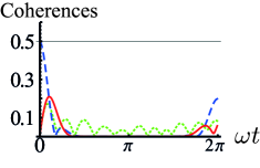
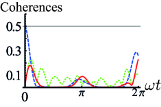
Figure 1: (color online): Coherences of the dimer’s density matrix for a chain affected by an environment prepared in a thermal and a squeezed-vacuum state [panel (a) and (b), respectively]. We have taken identical parameters for the two TLS-oscillator subsystems with $\hbar J=0.04$eV, $\hbar\omega=0.02$eV, $g=0.02$eV at room temperature ($T=293$ K). In this case $\alpha=1$. As explained in the text, the squeezing factor for the results in panel (b) has been taken so that the reduced single-oscillator state has the same effective temperature as in the thermal state case [i.e. panel (a)]. Quantitatively, $r=0.816$. A coherence revival at $t=\pi/\omega$ is present for a squeezed-vacuum environment: the presence of quantum correlations between the environmental modes fundamentally affects the dynamics of the TLS’s.

By initializing the first (second) TLS in the coherent superposition $\left|\text{in}\right\rangle_{1}{=}a|-\rangle_{1}+b|+\rangle_{1}$ with $|a|^{2}+|b|^{2}{=}1$ ($\left|\text{in}\right\rangle_{2}=\left|-\right\rangle_{2}$) and considering that $[\mathbf{H_{tot}},\sum^{2}_{j=1}\hat{\sigma}^{z}_{j}]=0$, the state $|+,+\rangle_{12}$ will stays unpopulated, while the probability to populate $|-,-\rangle_{12}$ remains constant. In Fig. 1 we plot the coherences of the density matrix of the two TLS’s affected by boson environments prepared in either uncorrelated thermal states or a squeezed-vacuum one. In order to perform a faithful comparison between such two cases, we have taken the squeezing parameter according to $\tanh r=e^{-\frac{\beta\hbar\omega}{2}}$ with the value of $\beta$ provided by the thermal-state environment. This ensures that the reduced single-oscillator state obtained from the squeezed-vacuum environment is a thermal state having the same temperature as the one considered in the genuinely thermal instance. In this way, we can nicely isolate the effect of the entanglement shared by the environmental oscillators.

Clearly, the revival of coherences at $t={\pi}/{\omega}$ is only due to the presence of correlations in the environment and an indication of a significant deviation of the state properties in such two different environmental preparations. Fig. 2 shows the purity $P(t)=\text{Tr}(\rho_{12}^{2})$ of the chain’s density matrix $\rho_{12}$ in both the thermal and squeezed case. We plot such a figure of merit against the intra-site coupling strength $J$ and the re-scaled interaction time $\omega{t}$. Quite reasonably, at values of $J$ that are comparable with the TLS-oscillator coupling, the differences between the thermal and squeezed-vacuum cases becomes very small. We can understand this by considering that, for decreasing values of $J$, the non-local interaction between the sites of the chain becomes less relevant than the local TLS-oscillator coupling. This implies that each TLS is strongly tied to its associated mode so that the local features of the oscillator environment become more preponderant than the non-local ones and the differences with a configuration of independent environmental states fades away. On the contrary, the inter-site tunnelling arising from a large value of $J$ makes the inter-mode entanglement relevant. Such differences manifest themselves in a rather distinct behavior of the properties of the TLS state.

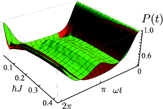
Figure 2: (Color online): Purity of dimer’s density matrix affected by individual environments prepared in a thermal state (red surface) and a squeezed-vacuum one (green surface, staying above the previous one). $P(t)$ is plotted against the chain inter-site coupling energy $\hbar J$ for $h\omega=0.04$eV, $g=0.02$eV and $T=293$K, which corresponds to $\alpha=1/2$. We have taken a squeezing factor $r=0.489$ (see text for further details on this choice).

As a special but very interesting case, we consider the chain to be initialized in the maximally entangled state ${({1}/{\sqrt{2}})(|--\rangle+|++\rangle)_{12}}$ and wonder about the behavior that entanglement has under the interaction model we are studying. Such an initial state is interesting on its own as, remarkably, it is relatively straightforward to find closed analytical expressions for the elements of the reduced TLS density matrix $\rho_{12}$.

(a)                                   (b)

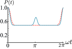
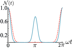
Figure 3: (Color online): Purity [panel (a)] and logarithmic negativity [panel (b)] of the state of a two-site chain initially prepared in the maximally entangled state $({1}/{\sqrt{2}})(|--\rangle+|++\rangle)_{12}$ and affected by either thermal states of the oscillator environment (red dashed curve) or an entangled squeezed-vacuum state (solid dark one) for $(\hbar J,\hbar\omega,g)=(0.1,0.01,0.005)$eV and $r=1.158$, corresponding to $\alpha=1/2$. The revival at $t=\pi/\omega$ associated with the squeezed-vacuum case is very pronounced.

While the populations of such matrix remain constant, the interesting element turns out to be the coherence $\langle++|\rho_{12}(t)|--\rangle$, for which we find

$$\langle++|\rho_{12}(t)|--\rangle{=}\dfrac{1}{2}e^{4i\epsilon t+8\alpha^{2}\frac{(\lambda_{\text{th}}^{2}+1)}{\lambda_{\text{th}}^{2}-1}[1-\cos(\omega t)]t}$$ (17)

for an oscillator environment prepared in the tensor product of two individual thermal states, while

$$\langle++|\rho_{12}(t)|--\rangle{=}\dfrac{1}{2}e^{4i\epsilon t+8\alpha^{2}\frac{1{+}\lambda_{\text{sq}}^{2}{+}2\lambda_{\text{sq}}\cos(\omega t)}{\lambda_{\text{sq}}^{2}-1}[1{-}\cos(\omega t)]t}$$ (18)

is valid for a squeezed-vacuum environment with ${\lambda_{\text{th}}=\lambda_{\text{sq}}^{2}=\overline{n}/(\overline{n}+1)}$.

The additional oscillatory term proportional to $\lambda_{\text{sq}}\cos\omega{t}$ appearing in Eq. (18) is responsible for the differences in the trend followed by the coherences corresponding to such two cases. The state purity is given by

$$P(t)=\dfrac{1}{2}+2|\langle++|\rho_{S}(t)|--\rangle|^{2},$$ (19)

which is reported in Fig. 3 (a) for the two different types of environmental states considered in this study, highlighting in a rather striking way how strongly the entanglement between the environmental oscillators affects the TLS’s properties. The purity revival at $t=\pi/\omega$ is also reflected in the behavior of the entanglement shared by the TLS’s. We use logarithmic negativity logneg as our entanglement measure. This is defined as ${\cal N}(t)=\log_{2}||\rho^{PT}_{12}||$ with $\rho^{PT}_{12}$ the partially transposed density matrix of the two TLS’s and $||\hat{A}||=\text{Tr}\sqrt{\hat{A}^{\dagger}\hat{A}}$ the trace norm of any operator $\hat{A}$. At $t=\pi/\omega$, ${\cal N}(t)$ goes from zero (the system experiences a sudden death of entanglement) to a rather large value.

The trend illustrated so far has features of independence from the specific instance of initial state considered for the dimer. We have studied the evolution of ${\cal N}(t)$ when the system is initialized in a separable state, finding qualitatively analogous behaviors of such figure of merit. For instance, Fig. 4 reports the results corresponding to a chain prepared as $(1/\sqrt{2})(\left|-\right\rangle+\left|+\right\rangle)_{1}\otimes\left|-\right\rangle_{2}$: entanglement builds up in the system (both the curves in Fig. 4 are such that ${\cal N}(0)=0$) and never disappears (we have considered a relatively small coupling between environments and chain). However, while the case corresponding to a thermal-state environment has a periodicity of $2\pi/\omega$, when a squeezing is present, a resurgence of entanglement occurs at half the thermal-state period.

Such effects can be linked to an enhanced non-Markovian nature of the TLS dynamics arising when considering entangled environmental oscillators. The analysis of this connection is the main aim of the following section.

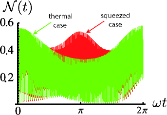
Figure 4: (Color online): Logarithmic negativity between the two sites of a chain affected by either thermal states of the oscillator environment (green curve) or an entangled squeezed-vacuum state (red one) for $r=0.816$ and $\alpha=1/4$. At $t=\pi/\omega$, ${\cal N}(t)$ has a revival, for the squeezed-vacuum case, which is absent from the thermal state-affected system.

II.1 Characterizing the non-Markovian nature of the dynamics

The quantification of the degree of non-Markovianity of adynamical evolution has been the focus of a significant recent research activity meas1 ; meas2 ; meas3 ; meas4 . The main goal of such investigation has been the identification of appropriate tools for the characterization of the many facets of non-Markovianity and the proposal of operational ways to quantify it. More recently, such tools have found application in the characterization of the memory-keeping evolution of systems of physical relevance app1 ; app2 . In this Subsection we move along such lines and employ one of the above-mentioned measures to determine the features of the dynamics under study here and the differences between the two environmental configurations addressed so far.

Quantitatively, we take inspiration from the measure of non-Markovianity proposed by Rivas et al. in Ref. meas2 , which is based on the following approach: consider a bipartite entangled state such that only one component of the bipartition is affected by the dynamics we would like to characterize. Then, by computing the amount of entanglement between the two parties at different instants of times within a selected interval $[t_{0},t_{\mathrm{max}}]$ we can detect non-markovianity by checking for a non-monotonic behavior of the quantum correlations. That is, for $\rho_{SA}(0)=|\Phi\rangle\langle\Phi|$ with $|\Phi\rangle$, some maximally entangled pure bipartite state, we define $\Delta E=E[\rho_{SA}(t_{0})]-E[\rho_{SA}(t_{\mathrm{max}})]$ (where $E$ denotes a legitimate entanglement monotone). We thus take

$$\mathcal{I}=\int_{0}^{t_{\mathrm{max}}}\left|\frac{dE[\rho_{SA}(t)]}{dt}\right|dt-\Delta E$$ (20)

If the evolution of the system is Markovian, the derivative of $E[\rho_{SA}(t)]$ is negative and $\mathcal{I}^{(E)}=0$.

While the measure in meas2 has been explicitly formulated for two qubits, so as to characterize the nature of a single-qubit channel, one can certainly think about extending the argument so as to address the case of a larger system. In particular, here we would like to be able to qualitatively understand the reasons behind the occurrence of the resurgence peak when an entangled environment is at hand.

Without embarking into the challenge of a rigorous formulation of the measure for non-Markovianity, we believe it is reasonable to consider the following situation: we take a genuinely tripartite entangled state of the two sites of the dimer at hand and an additional, ancillary TLS, which is exposed to a perfectly unitary dynamics (i.e. no environmental boson is interacting with the ancilla). More specifically, we consider the W state $(1/\sqrt{3})(\left|+--\right\rangle+\left|-+-\right\rangle+\left|--+\right\rangle)_{a12}$, which also ensures the presence of entanglement in any two-TLS reduction. While, as stated above, the ancilla $a$ undergoes a unitary evolution, particles $1$ and $2$ are exposed to the effective quantum channel described so far.

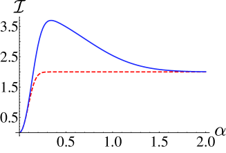
Figure 5: (Color online): Witness of non-Markovianity for the thermal (red dashed line) and squeezed blue solid line) case for $\hbar\omega=0.01$ and $r=1.15$ against the coupling strength $\alpha$.

We then apply Eq. (20), where $E$ is taken to be the logarithmic negativity between $a$ and the dimer, to the cases where the environment is prepared in a squeezed-vacuum and a two-mode thermal state. The results are shown in Fig. 5 against the effective coupling rate $\alpha=g/\hbar\omega$ for $t_{\text{max}}=2\pi/\omega$. While in the case of a thermal environment, ${\cal I}$ grows monotonically and saturates for $\alpha\gtrsim{0.4}$, for a squeezed-vacuum state it peaks at about this value of $\alpha$, signaling an increased non-Markovian behavior associated with such an environmental state. This magnified non-Markovianity is at the origin of the recurrence peaks exhibited in the analyses of the previous Sections. For lager coupling strengths $\alpha$, each TLS-environment interaction becomes so strong with respect to the inter-TLS one that the system fragments into a series of local sub-systems, each being basically oblivious to any non-local nature of the environmental state.

III Chain dynamics under a common environment

We now move to the study of a configuration where the TLS chain is affected by a common environment. The expression for the system-environment coupling given in the first line of Eq. (2) is thus modified into

$$\mathbf{\hat{H}_{SB}}=g\sum^{n_{o}}_{k=1}(\hat{a}_{k}+\hat{a}^{\dagger}_{k})\otimes\sum^{N}_{j=1}\hat{\sigma}^{z}_{j}$$ (21)

where we have assumed an oscillator environment consisting of $n_{o}$ modes, each identically coupled to all the TLS of and $N$-element chain. As remarked above, the symmetries in the present case are such that one can easily gather the exact analytical form of the evolved density matrix of the chain. For illustrative purposes, and to make a clear comparison to the case treated in previous Sections, we address a chain of two identical element, this time affected by a common environment composed by two boson modes. In Ref. Reina , an analogous problem has been approached by restricting the analysis to the single-excitation subspace and using a numerical method for the analysis of non-Markovian dynamics. Here, we shall pursue an analytic approach that is made possible by the analysis conducted in Sec. I

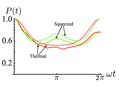
Figure 6: (Color online) Purity against dimensionless interaction time $\omega{t}$ for thermal (red) and squeezed (green) environment states, with $\hbar J=0.1,\hbar\omega=0.03,g=0.01,\alpha=1/3$ . In the two cases, squeezing parameter and (effective) temperature are $r=0.62$ and $T=293$ K. The dashed curves refer to the case of common environments.

(a)                                   (b)
  

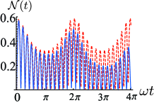
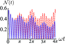
Figure 7: (Color online): Logarithmic Negativity for $\hbar J/g=0.2$ and $\alpha=1/3$, in the common- (dashed curve) and independent- (solid line) environment case. Panel (a) addresses the case of a thermal environment, while panel (b) is for a squeezed one.

We start by considering an arbitrary pure state $|\eta\rangle{=}{(a|-\rangle+b|+\rangle)}_{1}$ at site $1$ of the chain, while the second element is prepared in $|-\rangle_{2}$. The time evolution operator in the excitation-added displaced basis of the environmental modes is given by

$$\hat{\cal U}(t)=\sum_{n,m}e^{i\omega nt}\left(f(t)^{\pm}|\pm\pm\rangle\langle\pm\pm|\otimes|\alpha^{\pm\pm}_{n,m}\rangle\langle\alpha^{\pm\pm}_{n,m}|\right.$$ (22)

$$\left.+[\theta(t)|\mp\pm\rangle\langle\mp\pm|+h(t)|\mp\pm\rangle\langle\pm\mp|]\otimes|n,m\rangle\langle n,m|\right)$$

with $\varphi^{\pm}(t)=e^{\pm i(2\epsilon+\omega\alpha^{2})t}$, $\vartheta(t)=\cos(Jt)$ and $\kappa(t)=i\sin(Jt)$. Notice that, if $\alpha=0$, then $|\alpha^{\pm}_{n}\rangle=|n\rangle$. With this expression at hand, the reduced density matrix of the chain is

$$\rho_{12}(t){=}\begin{pmatrix}0&0&0&0\\ 0&b^{2}\vartheta^{2}(t)&b^{2}\vartheta(t)\kappa^{*}(t)&ab^{*}\varphi^{+}(t)\vartheta(t)\gamma(t)\\ 0&b^{2}\vartheta(t)\kappa(t)&b^{2}\kappa^{2}(t)&ab^{*}\varphi^{+}(t)\kappa(t)\gamma(t)\\ 0&a^{*}b\varphi^{-}(t)\vartheta(t)\gamma^{*}(t)&a^{*}b\varphi^{-}(t)\kappa^{*}(t)\gamma^{*}(t)&a^{2}\end{pmatrix}$$ (23)

where we have introduced the decoherence factor

$$\gamma(t)=\exp[{{-2\alpha^{2}\overline{n}(e^{i\omega t}-1)(e^{-i\omega t+\beta\omega}-1)}}]$$ (24)

for the thermal state case and

$$\gamma(t)= \exp[{-2\alpha^{2}\dfrac{(1-e^{-i\omega t})(1-e^{-i\omega t}\lambda_{\text{sq}}^{2})+[1-2\cos(\omega t)+\cos(2\omega t)]\lambda_{\text{sq}}}{\lambda_{\text{sq}}^{2}-1}}]$$ (25)

for squeezed-vacuum one.

Very similar features between the individual-environment and the common-environment cases are found by studying the behavior of purity. Fig. 6 shows that, regardless of the environmental configuration (whether made out of a common system or two individual oscillators), the squeezed-vacuum preparation is responsible for the revival of purity discussed above, a feature that is absent from the thermal case.

It is interesting to notice that the central block of the density matrix in Eq. (23) does not contain any decoherence factor, thus being fully decoherence-free: entanglement and purity will be preserved in time, in such a subspace, which is associated with a single excitation. Clearly, this marks a net difference with the case of two independent environments, where no such special symmetry exists. Such a distinction is evident from the inspection of Fig. 7, where we plot the logarithmic negativity in the common and individual-environment cases, for both the thermal and squeezed-vaccum preparation: the long-time behavior in the individual-environment arrangement clearly manifests a decrease of ${\cal N}(t)$ that is absent from the common-environment configuration.

IV Three-site chain: the role of the sharing-structure of environmental entanglement

After having analyzed in the previous Sections the basic building-block for any complex structure of interacting TLS’s, we move to the study of an open three-site chain (a trimer) affected by individual environments. While, qualitatively, the result gathered in Sec. II will be fully confirmed, such a scenario offers us an opportunity to investigate whether the sharing structure of the environmental entanglement plays any role in the open-system dynamics undergone by the TLS-chain.

To start with, we have considered the three-mode squeezed state $\left|\text{sq}_{3}\right\rangle{=}(1{-}\lambda^{2})^{-1/2}\sum^{3}_{l=0}\lambda^{l}\left|l,l,l\right\rangle_{123}$. This state is such that, upon tracing out one of the modes, the remaining two are fully separable thermal states, thus witnessing the GHZ-like nature of such state. We have found negligible differences in the dynamics of the trimer arising from the use of such environmental state or the tensor product $\otimes^{3}_{j=1}\rho_{\text{th},j}$: as shown in Fig. 8, for instance, the purity function $P(t)$ of the three-TLS state corresponding to such cases is very similar [as seen by inspecting the two bottom curves in Fig. 8]. The insensitivity to squeezing is confirmed by looking at the bipartite entanglement between any pair of chain elements achieved after tracing out one TLS-oscillator subsystem. Fig. 9 illustrates the behavior of the logarithmic negativity for such bipartite states; the results are valid, qualitatively, regardless of the pair being taken and show that there is no revival peak at $=\pi/\omega$ in the case of a squeezed environment. Moreover, a similar behavior is observed when considering the tripartite negativity, which is a legitimate entanglement monotone for the tripartite case trineg .

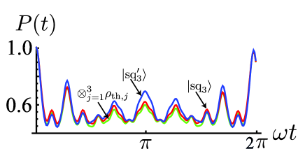
Figure 8: (Color online): Purity of three sites chain for the cases of thermal (green), generalized squeezed (red) and double split (blue) environment states. The nature of genuine tripartite entanglement of the generalized squeezed state is almost invisible, while some differences in the time evolution can be pointed out for the split squeezed state.

(a)                                               (b)                                               (c)

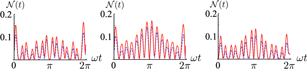
Figure 9: Bipartite logarithmic negativity ${\cal N}(t)$ against $\omega{t}$ for the reduced state of two TLSs’ obtained from a three-site chain by tracing out one of the particles. We have taken $\hbar{J}=0.2$eV, $\alpha=1/4$ with $r=0.488$ and $T=293$K. The solid (dashed) lines are for the squeezed (thermal) case. Panel (a), (b) and (c) show the results achieved when particle $1$, $2$ and $3$ are traced out, respectively.

The situation however changes if we modify the entanglement-sharing structure among the environmental oscillators. To show this fact, we have taken a three-mode state obtained by superimposing at a beam-splitter one mode of a squeezed state $\left|\text{sq}_{2}\right\rangle_{12}$ to an ancilla prepared in the vacuum state $\left|0\right\rangle_{3}$. More formally, we consider the state

$$\left|\text{sq}^{\prime}_{3}\right\rangle=(\openone_{1}\otimes\hat{B}_{23})(\theta)\left|\text{sq}_{2}\right\rangle_{12}\otimes\left|0\right\rangle_{3}$$ (26)

with $\hat{B}(\theta)=\exp[({\theta/2})(\hat{a}^{\dagger}_{2}\hat{a}_{3}-\hat{a}^{\dagger}_{3}\hat{a}_{2})]$ being the beam splitter operator of transmittivity $\cos^{2}(\theta/2)$ barnettradmore . For $\theta=0$ ($\theta=\pi$), a two-mode squeezed-vacuum state of modes $1$ and $2$ ($1$ and $3$) is retrieved, while for intermediate values of such parameter, an entangled three-mode state is achieved having non-separable two-mode reduced states. In this second case, the environmental entanglement visibly affects the global properties of the system in a way consistent with what we have seen earlier in Sec. II, see Fig. 8, thus reinforcing the idea that the structure of quantum correlations shared by the environmental oscillators plays a key role in the detailed non-Markovian dynamics of the TLS subsystem.

V Conclusions

We have studied the full non-Markovian dynamics of a system of interacting TLS’s arranged in a linear configuration and affected by a bosonic environment, considering both the individual and common-environment cases. By properly choosing the basis onto which each TLS-oscillator interaction is described, we have been able to push the analytic approach to such a problem up to the point of constructing a handy recipe for tracking any regime of interaction, from the weak to the strong-coupling regime with, in principle, an arbitrary number of environmental modes per site. This has paved the way to the study of the effects that quantum entanglement shared by the elements of the environment has on the dynamics of the TLS system. Entanglement appears to enhance the non-Markovian character of the evolution, giving rise to specific features in relevant figures of merit of a TLS chain that are not present in the case of uncorrelated environmental states. We have illustrated such effects by studying a dimer, which is the basic building-block for the construction of interesting interaction configurations that are usually considered for the description of biological complexes. Our investigation leaves open a series of questions related, in particular, to the scaling of the effects revealed here with the degree of connectivity, the depth and the geometry of the network of interacting TLS’s. We plan to address such issues by extending and improving the implementability of our method.

- (1) A. J. Leggett, S. Chakravarty, A. T. Dorsey, M. P. A. Fisher, A. Garg, and W. Zwerger, Rev. Mod. Phys. 59, 1 (1987).
- (2) J. Eckel, J. H. Reina and M. Thorwart, New J. Phys 11, 085001 (2009).
- (3) F. Caruso, A. W. Chin, A. Datta, S. F. Huelga and M. Plenio, Phys. Rev. A 81, 062338 (2010);
- (4) P. Rebentrost, M. Mohseni, I. Kassal, S. Lloyd, and A. Aspuru-Guzik, New J. Phys. 11 033003 (2009).
- (5) T. Scholak, et al., Phys. Rev. E 83, 021912 (2011).
- (6) F. Caruso, A. W. Chin, A. Datta, S. F. Huelga and M. Plenio, J. Chem. Phys. 131, 105106 (2009).
- (7) P. Rebentrost, R. Chakraborty, and A. Aspuru-Guzik, J. Chem. Phys. 131, 184102 (2009).
- (8) P. E. Barclay, K.-M. Fu, C. Santori, and R. G. Beausoleil, Optics Express 17, 9588 (2009); Appl. Phys. Lett. 95, 191115 (2009); P. E. Barclay, K.-M. C. Fu, C. Santori, A. Faraon, R. G. Beausoleil, arXiv:1105.5137; A. Faraon, P. E. Barclay, C. Santori, K.-M. C. Fu, and R. G. Beausoleil, Nat. Photon. 5, 301 (2011); C. Santori, P. E. Barclay, K.-M. C. Fu, S. Spillane, M. Fisch, and R. G. Beausoleil, Nanotechnology 21, 274008 (2010).
- (9) A. Wallraff, et al., Nature (London) 431, 162 (2004); M. Hofheinz, et al., Nature (London) 454, 310 (2008); J. M. Fink, et al., Nature (London) 454, 315 (2008); L. S. Bishop, et al., Nature Phys. 5, 105 (2009); O. Astafiev, et al., Science 327, 840 (2010); J. M. Fink, et al., Phys. Rev. Lett. 105, 163601 (2010); C. Lang, et al., Phys. Rev. Lett. 106, 243601 (2011).
- (10) J. Bourassa et al., Phys. Rev. A 80, 032109 (2009); A. Fedorov, A. K. Feofanov, P. Macha, P. Forn-Díaz, C. J. P. M. Harmans, and J. E. Mooij, Phys. Rev. Lett. 105, 060503 (2010); P. Forn-Díaz, J. Lisenfeld, D. Marcos, J. J. García-Ripoll, E. Solano, C. J. P. M. Harmans, and J. E. Mooij, Phys. Rev. Lett. 105, 237001 (2010); J. Casanova, G. Romero, I. Lizuain, J. J. García-Ripoll, and E. Solano, Phys. Rev. Lett. 105, 263603 (2010).
- (11) G. M. Palma, K.-A. Suominen, and A. Ekert, Proc. R. Soc. Lond. A 452, 567 (1996); J. H. Reina, L. Quiroga, and N. F. Johnson, Phys. Rev. A 65, 032326 (2002).
- (12) S. M. Barnett and P. M. Radmore, Methods in Theoretical Quantum Optics (Oxford University Press, New York, 1997).
- (13) M. Abramowitz and I. Stegun, Handbook of Mathematical Functions with Formulas, Graphs, and Mathematical Tables (Dover, New York, 1964).
- (14) One can relate the Charlier polynomials to the associated Laguerre polynomials as , where is a generic argument.
- (15) M. B. Plenio, Phys. Rev. Lett. 95, 090503 (2005).
- (16) M. M. Wolf, J. Eisert, T. S. Cubitt, and J. I. Cirac, Phys. Rev. Lett. 101, 150402 (2008).
- (17) A. Rivas, S. F. Huelga, and M. B. Plenio, Phys. Rev. Lett. 105, 050403 (2010); D. Chruscinski, A. Kossakowski, and A. Rivas, Phys. Rev. A 83 5 (2011).
- (18) H.-P. Breuer, E. M. Laine, and J. Piilo, Phys. Rev. Lett. 103, 210401 (2009); E.-M. Laine, J. Piilo, and H.-P. Breuer, Phys. Rev. A 81, 062115 (2010).
- (19) X.-M. Lu, X. Wang, and C. P. Sun, Phys. Rev. A 82, 042103 (2010).
- (20) T. J. G. Apollaro, C. Di Franco, F. Plastina, M. Paternostro, Phys. Rev. A 83, 032103 (2011).
- (21) P. Haikka, S. McEndoo, G. De Chiara, M. Palma, and S. Maniscalco, arXiv:1105.4790 (2011).
- (22) The tripartite negativity is defined as , with the negativity in the bipartition.