Herschel observations of the Herbig-Haro objects HH 52-54

Abstract

Context. The emission from Herbig-Haro objects and supersonic molecular outflows is understood as cooling radiation behind shocks, initiated by a (proto-)stellar wind or jet. Within a given object, one often observes the occurrence of both dissociative (J-type) and non-dissociative (C-type) shocks, owing to the collective effects of internally varying shock velocities.

Aims. We are aiming at the observational estimation of the relative contribution to the cooling by CO and H₂O, as this provides decisive information for the understanding of the oxygen chemistry behind interstellar shock waves.

Methods. The high sensitivity of HIFI, in combination with its high spectral resolution capability, allows us to trace the H₂O outflow wings at unprecedented signal-to-noise. From the observation of spectrally resolved H₂O and CO lines in the HH52-54 system, both from space and from ground, we arrive at the spatial and velocity distribution of the molecular outflow gas. Solving the statistical equilibrium and non-LTE radiative transfer equations provides us with estimates of the physical parameters of this gas, including the cooling rate ratios of the species. The radiative transfer is based on an Accelerated Lambda Iteration code, where we use the fact that variable shock strengths, distributed along the front, are naturally implied by a curved surface.

Results. Based on observations of CO and H₂O spectral lines, we conclude that the emission is confined to the HH54 region. The quantitative analysis of our observations favours a ratio of the CO-to-H₂O-cooling-rate $\gg 1$. Formally, we derive the ratio $\Lambda({\rm CO})/\Lambda$(o-H₂O) $=10$, which is in good agreement with earlier determination of 7 based on ISO-LWS observations. From the best-fit model to the CO emission, we arrive at an H₂O abundance close to $1\times 10^{-5}$. The line profiles exhibit two components, one of which is triangular and another, which is a superposed, additional feature. This additional feature likely originates from a region smaller than the beam where the ortho-water abundance is smaller than in the quiescent gas.

Conclusions. Comparison with recent shock models indicate that a planar shock can not easily explain the observed line strengths and triangular line profiles. We conclude that the geometry can play an important role. Although abundances support a scenario where J-type shocks are present, higher cooling rate ratios than predicted by these type of shocks are derived.

1 Introduction

Outflows have many times been discovered through observations of Herbig-Haro objects (see e.g. Herbig, 1950, 1951; Haro, 1952, 1953), tracing the gas at highest velocity. Liseau & Sandell (1986) showed that HH-objects and outflows are physically associated, implying that they likely have the same exciting source.

Water is one of the coolants that is most sensitive to different type of shock chemistry (e.g. Bergin et al., 1998). Depending on the ionisation fraction, magnetic field strength and velocity of the shock, water abundances can be elevated to different levels (Hollenbach et al., 1989). In J-type shocks (Jump shocks), where the magnetosonic speed is lower than the propagation of the pressure increase, the involved energies generally dissociate H₂ and all molecules with lower binding energies. As such the water abundance is generally low in J-type shocks, although it may reform in the post-shock cooling region once pre-shock densities are sufficiently high. In C-type shocks however, the pre-shock gas is partially heated due to traversing magnetic waves from the post-shock gas, and molecules can survive the passage of the shock (Draine, 1980) where both the magnetic field and the gas density is compressed. In this type of shock, the activation barrier for neutral-neutral reactions between molecular hydrogen and oxygen is reached, and the water abundance is expected to become enhanced. This can be both due to the effect of sputtering from dust grains (Kaufman & Neufeld, 1996) and due to high temperature chemistry occurring

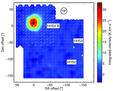
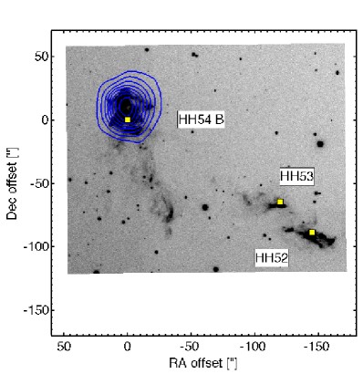
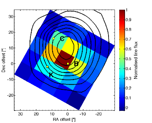
Figure 1: Upper panel: False colour map of the CO (10$-$9) integrated intensity in the blue line wing (from $+$2.4 $\mathrm{km\,s^{-1}}$ to $-$30 $\mathrm{km\,s^{-1}}$). The positions of HH 54 B, HH 53 and HH 52 are indicated with yellow squares. The readout positions for the on-the-fly and raster maps are indicated with white dots.
Middle panel: CO (10$-$9) map of the integrated intensity obtained with HIFI in the blue line wing overlaid on an H$\alpha$ image from Caratti o Garatti et al. (2009). Contours are from 5.5 to 33.6 K $\mathrm{km\,s^{-1}}$ in steps of 3.5 K $\mathrm{km\,s^{-1}}$.
Lower panel: A zoom of the CO (10$-$9) integrated intensity overlaid on the $\rm{H_{2}O\,(2_{12}-1_{01})}$ emission obtained with PACS. The positions of HH 54 B, C and K as indicated in Giannini et al. (2006) are indicated with yellow squares.

in the shocked region (Bergin et al., 1998). After the shock passage, the enhanced water abundance persists for a long time in the post-shock gas.

The atmosphere of the Earth is opaque at the wavelength of the lowest rotational transitions of water as well as most other higher excited transitions. Thus, it is not until recent years, with the use of space based observatories, these transitions have been observed successfully. Previous missions such as SWAS (Melnick et al., 2000) and Odin (Nordh et al., 2003) have put constraints on the water abundance and the dynamics of molecular outflows (Franklin et al., 2008; Bjerkeli et al., 2009). None of these missions, however, provided the spatial and spectral resolution that is available with the Herschel Space Observatory (Pilbratt et al., 2010).

HH 54 is a Herbig-Haro object located in the Chamaeleon II cloud at a distance of approximately 180 pc (Whittet et al., 1997). The visible objects in HH 54 are moving at high Doppler speed out of the cloud toward the observer, with velocities of the order 10 - 100 $\mathrm{km\,s^{-1}}$ (Caratti o Garatti et al., 2009). The objects show a clumpy appearance due to either Rayleigh-Taylor instabilities in the flow or due to variability in the jet itself. Another possibility is patchy overlying dust extinction. The source of the jet is not well constrained. This is further discussed in appendix A.2, where we also present quantitative arguments for identifying IRAS 12553-7651 (ISO-Cha II 28) as the HH54 jet-driving source and its associated blueshifted CO outflow. No redshifted emission is observed as what would be expected from a bipolar jet (see Section 3). On the other hand, the extinction is relatively low, something that might allow the redshifted gas to flow out essentially unhindered into the low density material at the rear side of the cloud. It can however not be ruled out that the outflow itself is one-sided and asymmetric. Recent simulations show that rapidly rotating stars with complex magnetic fields can be responsible for such type of flows (Lovelace et al., 2010).

HH 54 has previously been observed in various lines of CO, SiO and H₂O using Odin and SEST (Bjerkeli et al., 2009, R. Liseau, unpublished). Several H₂O lines and high-J CO lines were also observed with ISO-LWS and published in Liseau et al. (1996) and Nisini et al. (1996). During the Performance Verification Phase of the Heterodyne Instrument for the Far-Infrared (HIFI) instrument, aboard the Herschel Space Observatory, the CO (10$-$9) transition was observed. As part of the WISH keyprogram (van Dishoeck et al., 2011), also the $\rm{H_{2}O\,(1_{10}-1_{01})}$ and $\rm{H_{2}O\,(2_{12}-1_{01})}$ transitions were observed using HIFI and the Photodetector Array Camera and Spectrometer (PACS) respectively. We note that the wavelength region, covering the $\rm{H_{2}O\,(2_{12}-1_{01})}$ transition, also can be observed with HIFI.

In this paper, we present observations, both from space and ground, of HH 52-54 in spectral lines of CO and H₂O. We choose to observe this region based on the fact that HH54 is free from contamination from other objects, spatially confined and resolved in the infrared regime with the instruments used. Using results from observations carried out with SEST, APEX, Odin and Herschel, we aim at improving our understanding of interstellar shock waves. The observing modes and the instruments that have been used are described in Section 2 while the details of the HIFI data reduction can be found in Appendix B. The basic observational results are summarised in Section 3 whereas the interpretations are discussed in Section 4.

Table 1: Molecular line observations carried out with Odin, SEST, APEX and Herschel.

Telescope	Molecule	Frequency	$E_{u}/k_{\rm{B}}$	HPBW	$\eta_{\rm{mb}}$	Date	$t_{\textrm{\tiny int}}$
		(GHz)	(K)	(′′)		(YYMMDD)	(hr)
SEST	CO (2$-$1)	230.538	16.6	23	0.50	970811 - 980806	3
SEST	CO (3$-$2)	345.796	33.2	15	0.25	970811 - 980806	3
APEX	CO (4$-$3)	461.041	55.3	14	0.60	070918	0.5
Odin	CO (5$-$4)	576.268	83.0	118	0.90	050502 - 050620	4
APEX	CO (7$-$6)	806.652	155.9	8	0.43	070918	0.8
Herschel-HIFI	CO (10$-$9)	1151.985	304.2	19	0.66	090726 - 100221	9
Odin	$\rm{H_{2}O\,(1_{10}-1_{01})}$	556.936	42.4	126	0.90	090609 - 100420	12
Herschel-HIFI	$\rm{H_{2}O\,(1_{10}-1_{01})}$	556.936	42.4	39	0.76	100729	0.05
Herschel-PACS	$\rm{H_{2}O\,(2_{12}-1_{01})}$	1669.905	79.5	13	N/A	090226	0.1

2 Observations

The observations described in this paper were obtained between 1997 and 2010 with several different facilities. A summary of the observations is presented in Table 1 while the line intensities are listed in Table 2.

2.1 Herschel

2.1.1 HIFI

During the Performance Verification Phase of HIFI (de Graauw et al., 2010), the CO (10$-$9) data were obtained on 26-27 July 2009 and 21 February 2010. The H₂O data were obtained 29 July 2010. The 3.5 m Cassegrain telescope has a Full Width Half Maximum (FWHM) of 38^′′ at 557 GHz, 19^′′ at 1152 GHz and 13^′′ at 1670 GHz, respectively. The HIFI $\rm{H_{2}O\,(1_{10}-1_{01})}$ spectrum presented in this paper was obtained in point mode with position switch using band 1 (490 - 630 GHz). The OFF spectrum is obtained by a single observation of a reference point 10^′ away. The CO (10$-$9) HIFI maps were obtained in two different observing modes using band 5 (1120 - 1250 GHz). In the dual-beam-switch raster mode, an internal chopper mirror is used to obtain an OFF spectrum 3^′ away from the observed position. In the on-the-fly with position switch mode, the telescope is scanning the map area back and forth. The data were calibrated using the Herschel Interactive Processing Environment (HIPE) version 4.2 and 5.0 for the CO (10$-$9) and $\rm{H_{2}O\,(1_{10}-1_{01})}$ observations, respectively (Ott, 2010). The data reduction of the HIFI maps is described in detail in Appendix B. For the CO (10$-$9) observation, data from one of the spectrometers on-board have been used. The Wide Band Spectrometer (WBS) is an acousto-optical spectrometer with a 4 GHz frequency coverage. The channel spacing is 500 kHz (0.1 $\mathrm{km\,s^{-1}}$ at 1152 GHz and 0.3 $\mathrm{km\,s^{-1}}$ at 557 GHz). For the $\rm{H_{2}O\,(1_{10}-1_{01})}$ observation, data from the High Resolution Spectrometer (HRS) have also been used. The HRS is an Auto-Correlator System (ACS) where the resolution can be varied from 0.125 - 1.00 MHz. For this observation it was set to 0.24 MHz. Observations from the horizontal (H) and the vertical (V) polarisations were combined for both observations. The spectra were converted to a $T_{\rm mb}$ scale using main beam efficiencies, $\eta_{\mathrm{mb}}(1152\mathrm{GHz})$ = 0.66 and $\eta_{\mathrm{mb}}(557\mathrm{GHz})$ = 0.76 (Olberg, 2010).

2.1.2 PACS

The PACS spectrograph (Poglitsch et al., 2010) is a 5$\times$5 integral field unit array consisting of $9\aas@@fstack{\prime\prime}4$ square spaxels (spatial picture elements). The observations were obtained on 26 February 2009 in line scan mode and cover the 178.8–180.5 $\mu$m region, centered on the $\rm{H_{2}O\,(2_{12}-1_{01})}$ line at 179.5 $\mu$m. The blue channel simultaneously covered the 89.4–90.2 $\mu$m region, which is featureless and not discussed further. Two different nod positions, located 6^′ from the target in opposite directions, were used to correct for the telescopic background. Data were reduced with HIPE version 4.0. The fluxes were normalised to the telescopic background and subsequently converted to an absolute flux based on PACS observations of Neptune (Lellouch et al., 2010), with an approximate uncertainty of $\sim$20 % at 180 $\mu$m. The spatial resolution at 180 $\mu$m is nearly diffraction-limited (see Table 1). In well-centered observations of point sources, only about 40 % of the light in the system falls within the central spaxel. The $\rm{H_{2}O\,(2_{12}-1_{01})}$ line is spectrally unresolved in the $R=1700$ spectra ($\Delta\upsilon$ $\sim$ 175 $\mathrm{km\,s^{-1}}$).

2.2 Odin

The Odin space observatory carries a 1.1 m Gregorian telescope and was launched into space in 2001 (Nordh et al., 2003; Hjalmarson et al., 2003). It is located in a polar orbit at 600 km altitude. At 557 and 576 GHz, the FWHM is 126^′′ and 118^′′ respectively. The spectra were converted to a $T_{\rm mb}$ scale using a main beam efficiency, $\eta_{\mathrm{mb}}$ = 0.9, as measured from Jupiter observations (Hjalmarson et al., 2003).

The CO (5$-$4) observations, suffered from frequency drift and have, for that reason, been calibrated, using atmospheric spectral lines, acquired during the time intervals when Odin observed through the Earth’s atmosphere (Olberg et al., 2003). Since the first publication of the CO (5$-$4) data in Bjerkeli et al. (2009), the frequency calibration scheme has improved. Despite this, the velocity scale for this particular observation has some uncertainties due to in-orbit variations of the local oscillator unit frequency. These variations are most likely caused by slight temperature changes in the spacecraft during each orbit, due to the fact that the Earth is located very nearby. On a velocity scale these fluctuations correspond to a $\sim$2 $\mathrm{km\,s^{-1}}$ uncertainty.

A spectrum, showing a tentative detection of $\rm{H_{2}O\,(1_{10}-1_{01})}$ at 557 GHz was published in Bjerkeli et al. (2009). Since then, however, additional observations toward HH 54 have been carried out in June 2009 and April 2010 for a total on-source time of 12 hours.

The observing mode for both observations was position switching, where the entire telescope is re-orientated to obtain a reference spectrum (10^′ away in June 2009 and 15^′ away in April 2010). The spectrometer used is an acousto-optical spectrometer (AOS) where the channel spacing is 620 kHz (0.33 $\mathrm{km\,s^{-1}}$ and 0.32 $\mathrm{km\,s^{-1}}$ at 557 GHz and 576 GHz respectively). The data processing and calibration are described by Olberg et al. (2003).

2.3 SEST

The observations and calibration of the CO (2$-$1), CO (3$-$2), SiO (2$-$1), SiO (3$-$2) and SiO (5$-$4) data obtained with SEST were already described in detail by Bjerkeli et al. (2009), to which we refer the interested reader.

2.4 APEX

CO (4$-$3) and CO (7$-$6) data were obtained with the APEX/FLASH receiver in service mode in July 2006. In this project, both CO lines were observed simultaneously in a grid map around HH54 B centered on $\alpha_{2000}$ = 12^h55^m49$\stackrel{{{}^{\rm s}}}{{{}_{\bf\cdot}}}$5, $\delta_{2000}$ = $-$76^∘56^′23^′′. The selected reference position was relatively nearby at (120^′′,$-$120^′′), which resulted in contaminated line spectra close to the cloud LSR velocity (see below). The telescope pointing was checked by observing the nearby nova X Tra (IRAS 15094-6953). The map was spaced by half the instrument beam for the CO (4$-$3) transition which corresponds to 7^′′ at 450 GHz. The data reduction was performed in CLASS and the spectra were converted to a $T_{\rm mb}$ scale using the main beam efficiencies, 0.60 and 0.43 for the CO (4$-$3) and CO (7$-$6) transitions, respectivelly (Güsten et al., 2006). The channel spacing is 61 kHz (0.04 $\mathrm{km\,s^{-1}}$ at 461 GHz and 0.02 $\mathrm{km\,s^{-1}}$ at 807 GHz).

3 Results

The results from our observations are summarised in Table 2, where the integrated intensity over the blue line wing is presented.

Table 2: Integrated intensities over the line wings and 1 $\sigma$
uncertainties in parentheses.

Line	Source	$\Delta$$\upsilon_{\rm LSR}$	$\int\!T_{\rm{mb}}\leavevmode\nobreak\$$d\upsilon$	$T_{\rm{mb,rms}}$a
		($\rm{km\leavevmode\nobreak\ s^{-1}}$)	($\rm{K\leavevmode\nobreak\ km\leavevmode\nobreak\ s^{-1}}$)	(mK)
CO (2$-$1)	HH 54	0.9 to $-23.3$	34.6 (0.3)	224
CO (3$-$2)	HH 54	0.9 to $-23.3$	54.9 (1.9)	2021
CO (4$-$3)	HH 54	2.4 to $-23.3$	104.4 (3.9)	773
CO (5$-$4)	HH 54	2.4 to $-21.8$	9.3 (0.06)	20
CO (7$-$6)	HH 54	2.4 to $-21.8$	128.1 (25.3)	4741
CO (10$-$9)	HH 52	-	-	284
	HH 53	-	-	211
	HH 54	2.4 to $-21.8$	33.1 (0.3)	146
$\rm{H_{2}O\,(1_{10}-1_{01})}$b	HH 54	2.4 to $-22.8$	9.2 (0.06)	20

Notes to the Table: ^aThe velocity bin size when calculating the rms is the same as the channel spacing. ^bThis refers to the spectra obtained with HIFI.

3.1 Herschel

CO (10$-$9) is only detected in the HH 54 region. No emission is detected toward the region of HH 52-53 down to an rms level of $\sim$0.2 K (see upper panel of Fig. 1) and these objects will not be discussed further. From the CO (10$-$9) emission, we estimate the size of the source to $\sim$27^′′. The $\rm{H_{2}O\,(1_{10}-1_{01})}$ line is clearly detected toward HH 54 (see Fig. 2). Simultaneously, the NH${}_{3}(1_{0}-0_{0})$ line at 572 GHz was covered in the upper side band. No emission is detected down to an rms level of $\sim$20 mK. For the $\rm{H_{2}O\,(2_{12}-1_{01})}$ line observed with PACS, emission is detected in most of the spaxels and the angular extent of the source is no larger than $\sim$28^′′. The peak flux in the central spaxel is 9 Jy.

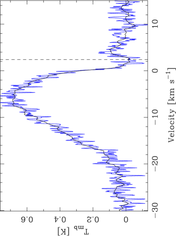
Figure 2: $\rm{H_{2}O\,(1_{10}-1_{01})}$ spectra obtained with HIFI. The blue spectral line is the HRS and the black spectral line is the WBS. Both observations were centered on HH 54 B: $\alpha_{2000}$ = 12^h55^m50$\stackrel{{{}^{\rm s}}}{{{}_{\bf\cdot}}}$3, $\delta_{2000}$ = $-$76^∘56^′23^′′. The dashed line indicates the position of the velocity of the cloud.

Figure 3: CO (10$-$9) map obtained with HIFI. The map shows the spectra toward the region close to HH 54 B and the map has been regridded with map spacing equal to $9\aas@@fstack{\prime\prime}3$. Offsets are with respect to HH 54 B: $\alpha_{2000}$ = 12^h55^m50$\stackrel{{{}^{\rm s}}}{{{}_{\bf\cdot}}}$3, $\delta_{2000}$ = $-$76^∘56^′23^′′. The velocity scale ($\upsilon_{\rm LSR}$) and intensity scale ($T_{\rm{mb}}$) is indicated in the upper right corner of the map, $\upsilon_{\rm LSR}$ = +2.4 $\mathrm{km\,s^{-1}}$ with a dashed line.

In the lower panel of Figure 1, the CO (10$-$9) integrated intensity contours are shown overlaid on the $\rm{H_{2}O\,(2_{12}-1_{01})}$ normalised flux in each spaxel. In this figure, each spaxel is presented on a square grid. In reality however, there is a small misalignment between each spaxel (see Poglitsch et al., 2010, Their Fig 10). An offset of $\sim$9^′′ between the CO (10$-$9) and the $\rm{H_{2}O\,(2_{12}-1_{01})}$ emission peak is also observed, where the peak of the CO emission is located in between the B and C clumps as identified by Sandell et al. (1987). This offset might be real given a pointing accuracy of a few arcseconds for Herschel. Noteworthy is that the different clumps in the region show detectable proper motion over a time scale of a few years (e.g. Schwartz et al., 1984; Caratti o Garatti et al., 2006, 2009). However, the CO and H₂O observations with Herschel were obtained over a time span of only one year and it is therefore unlikely that proper motion is the cause of the observed offset. The $\rm{H_{2}O\,(1_{10}-1_{01})}$ spectra obtained with HIFI are presented in Fig. 2. The line is self absorbed by the foreground cloud at $\upsilon_{\rm LSR}$ = +2.4 $\mathrm{km\,s^{-1}}$.

3.2 Odin

The Odin $\rm{H_{2}O\,(1_{10}-1_{01})}$ observations carried out on 9 June 2009 and 20 April 2010 confirmed the previously published detection with an improved signal to noise. It is this dataset that is used for the comparison with HIFI data in the present paper.

3.3 SEST

The CO (2$-$1) and CO (3$-$2) maps were centered with a slight offset with respect to HH 54 B, viz $4\aas@@fstack{\prime\prime}8$. The spacing in CO (2$-$1) was 25^′′while the spacing between the observations in CO (3$-$2) were of the order 15^′′, i.e one full beam width. The number of positions observed in the CO (2$-$1) map and the quality of the baselines in the CO (3$-$2) does not allow us to put constraints on the source size. SiO was not detected, when averaging all spectra together, down to an rms level of 10 mK for SiO (2$-$1), 15 mK for SiO (3$-$2) and 7 mK for SiO (5$-$4). The SEST data are presented in Fig. 4.

Figure 4: Same as Figure 3, but for the CO (2$-$1), CO (3$-$2), CO (4$-$3) and CO (7$-$6) maps obtained with SEST and APEX. The APEX maps have been regridded with a map spacing equal to 8^′′ for CO (4$-$3) and 9^′′ for CO (7$-$6). Note that the CO (4$-$3) spectra may be contaminated with OFF beam contribution.

3.4 APEX

The quality of the FLASH data is not fully satisfactory, as they suffer from off-beam contamination near the line centre. However, as we here are mainly focussing on the line wings, this should affect our conclusions only little, if at all. In these CO line maps, a bump feature (See Sec. 4.1) in the line profile was detected in some positions (at $\upsilon_{\rm LSR}$ = $-$7 $\mathrm{km\,s^{-1}}$, see below). A reliable source size from these maps can however not be determined. In both maps, the feature is detected in a velocity range spanning over $\Delta\upsilon$ $\simeq$ 7 $\mathrm{km\,s^{-1}}$ (see Fig. 4) .

4 Discussion

4.1 Observed line profiles

Common to the observed transitions in CO and H₂O is that only blue-shifted emission is detected. For all transitions, the maximum detected velocity in the line wing is of the order of $-20$ $\mathrm{km\,s^{-1}}$. A bump-like feature at $\upsilon_{\rm LSR}$ $\eqsim-7$ $\mathrm{km\,s^{-1}}$ is also clearly visible in the observed CO (10$-$9) and CO (2$-$1) spectra and possibly also in the CO (3$-$2), CO (5$-$4) and $\rm{H_{2}O\,(1_{10}-1_{01})}$ data. In the CO (10$-$9) map, this feature is more prominent in some positions than others, and most likely it is spatially unresolved to Herschel (see Fig 3). The $\upsilon_{\rm LSR}$ $\simeq-7$ $\mathrm{km\,s^{-1}}$ component is also clearly visible in the CO (4$-$3) and CO (7$-$6) spectra observed with APEX (see Figure 4) where the beam sizes are 13^′′ and 8^′′, respectively. Also in these maps, this component seems unresolved, hence it likely originates from a region with an angular extent that is smaller than the telescope beams. In the CO (5$-$4) data, where the beam size is 118^′′, the bump-like feature is barely visible. This is expected if the beam filling factor is small. A position-velocity diagram of the CO (10$-$9) transition shows a trend of higher velocities being detected at lower declination and closer to the position of HH 54 B (see Figs. 3 and 5), i.e where the $\rm{H_{2}O\,(2_{12}-1_{01})}$ emission peaks (see Fig. 1). This is also clearly visible in the right panel of Fig. 5 where the integrated intensity of the bump is presented together with the integrated intensity for the underlying triangular profile. The intensity maximum of the bump seems offset by $\sim$10^′′ to the south from the peak of the bulk outflow emission. The uncertainty attributed to this offset due to the baseline subtraction is of the order $\sim$5^′′.

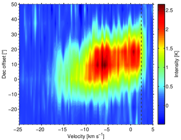
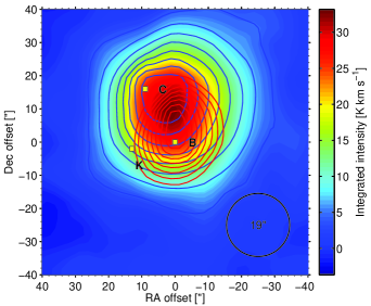
Figure 5: Left panel: Position (in DEC) velocity diagram of the HIFI CO (10$-$9) data showing the observed intensity. The bump-like feature can be seen at $\upsilon_{\rm LSR}$ = $-$7 $\mathrm{km\,s^{-1}}$. The offset in RA is 0 ^′′. $\upsilon_{\rm LSR}$ =$+$2.4 $\mathrm{km\,s^{-1}}$ is indicated with a dashed line.
Right panel: Blue contours are the integrated intensity when the bump-like feature is subtracted from the spectra. Contours are from 3.6 to 28.7 K $\mathrm{km\,s^{-1}}$ in steps of 3.1 K $\mathrm{km\,s^{-1}}$. Red contours show the integrated intensity for the bump. Contours are from 2.6 to 7.5 K $\mathrm{km\,s^{-1}}$ in steps of 0.6 K $\mathrm{km\,s^{-1}}$. Underlying colors show the total integrated intensity over the observed line. The positions of HH 54 B, C and K are indicated with yellow squares.

Assuming that the apex of the shock is located close to the HH54 B position, one would also expect the highest velocities in this region.

4.2 Interpretation of the emission line data

To compute the line profiles for the observed emission, we use an Accelerated Lambda Iteration (ALI) code (See App. C). The ALI code we use is a non-LTE, one dimensional code, assuming spherical geometry where several subshells are used. The number of cells and angles used in the ray tracing can also be arbitrarily chosen. In this work, a curved geometry is compared with a plane parallel slab to interpret the observed spectral lines.

The formation of the observed spectral lines occurs most likely in shocked gas. Using results from detailed models of C-shocks, Neufeld et al. (2006) presented estimates of the excitation conditions for HH 54. From the analysis of H₂-rotation diagrams, Neufeld et al. (2006) determined the presence of two different temperature regimes, viz. at 400 K and at 10³ K, respectively.

We used their analytical expressions for the column density,

$$N(\mathrm{H_{2}})=7.9\times 10^{20}\left[\frac{n(\mathrm{H_{2}})}{10^{5}}\right]^{0.5}\left(\frac{T_{\mathrm{gas}}}{1000}\right)^{-0.555}\leavevmode\nobreak\ \mathrm{cm^{-2}},$$ (1)

and for the velocity gradient,

$$\frac{d\upsilon}{dz}=1.6\times 10^{4}\left[\frac{n(\mathrm{H_{2}})}{10^{5}}\right]^{0.5}\left(\frac{T_{\mathrm{gas}}}{1000}\right)^{1.30}\leavevmode\nobreak\ \mathrm{km\leavevmode\nobreak\ s^{-1}\leavevmode\nobreak\ pc^{-1}}.$$ (2)

to compute the emission in the CO and H₂O lines. Here $n(\rm H_{2})$ is the pre-shock density and the other quantities have their usual meaning. Following Neufeld et al. (2006) we take the compression factor of 1.5, which was used by them for H₂, but we assume that holds for CO as well. In addition, they assume that the fractional beam filling of the two-temperature components is given by the ratio of the column density derived from the rotation diagram and that given by Eq. 1.

For these two temperatures, and for pre-shock densitites of 10⁴ cm^-3 and 10⁵ cm^-3, we compute from, Eqs. (1) and (2) in slab geometry, the emission in CO and H₂O lines, including the shapes of the lines. Other parameters (such as CO abundance, source size, microturbulence etc.) are given in Table LABEL:table:1. For the H₂O abundance we assume $X$($\mathrm{H_{2}O}$) = 1.0$\,\times\,10^{-5}$, consistent with the upper limit of $<$ 2$\,\times\,10^{-5}$ determined by Neufeld et al. (2006).

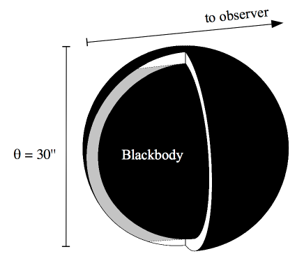
Figure 6: A cut through the shells of the spherical model described in the text. Essentially all radiation originating from the rear side of the sphere (grey) is blocked out by the central blackbody source.

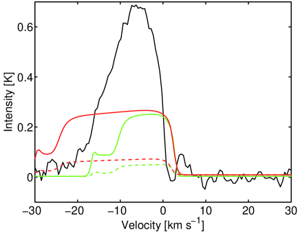
Figure 9: The red (1000 K) and green (400 K) lines represent the model described in Neufeld et al. (2006), using pre-shock densities of 10⁴ cm^-3 (dashed) and 10⁵ cm^-3 (solid). The observed spectrum for the $\rm{H_{2}O\,(1_{10}-1_{01})}$ transition with HIFI is plotted with a black solid line. The o-H₂O abundance is set to $X(o$-$\mathrm{H_{2}O})$ = 1$\,\times\,10^{-5}$.

The results are presented in Figs. 7 and 9. As seen in the latter figure, the computed line strength of the ground state line of o-H₂O for a temperature of 400 K and pre-shock density of 10⁵ cm^-3 is not far from what HIFI has observed. On the other hand, such parameters are not in agreement with the observed CO (10$-$9) line, the intensity of which is severely over-predicted. As expected, the low-J lines CO (2$-$1) and CO (3$-$2) are not very sensitive to the changes in temperature from 400 to 1000 K. In all cases the computed rectangular line shape is different from the observed profiles, which have a pronounced triangular shape.

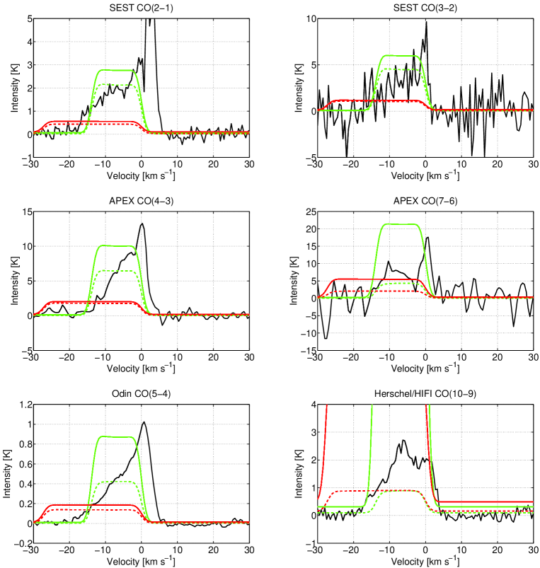
Figure 7: The red (1000 K) and green (400 K) lines represent the model described in Neufeld et al. (2006), using pre-shock densities of 10⁴ cm^-3 (dashed) and 10⁵ cm^-3 (solid). The observed spectra from SEST, APEX, Odin and HIFI are plotted with black solid lines. Note that the modelled spectra, not have been baselines subtracted.

4.3 Emission from a curved geometry

The spatial distribution of the gas does also influence the observed line profiles (see e.g. Hartigan et al., 1987). For that reason we also investigate a scenario where the emission originates from a curved geometry. To implement this we use a simple model that mimics an expanding shell with a diameter of 30^′′ located at a distance of 180 pc (see Fig 6). The interior of the spherical shell is empty, i.e. at the temperature of cosmic background radiation field. This cold sphere occupies 88% of the radius of the sphere, based on a shell thickness of 5$\,\times\,10^{15}$ cm. This value is in between the slab thickness estimated by Liseau et al. (1996) and the analytical expression for the slab thickness at 180 K. The shell thickness is also consistent with the cooling length estimated by Kaufman & Neufeld (1996). Using this method, we block out essentially all the radiation originating from the opposite side of the sphere.

To compare with the observed line profiles, spectra are computed viewing the curved surface from the front. This is supported by the absence of detectable SiO emission which is often observed in molecular outflows with relatively high velocities (see e.g. Nisini et al., 2007). Shock modelling carried out by Gusdorf et al. (2008) suggests that sputtering is not very efficient in the velocity regime below 25 $\mathrm{km\,s^{-1}}$. Therefore, assuming that the outflow in HH 54 is observed from the front, and that it has a small inclination angle with respect to the line of sight, the maximum velocity of the molecular gas is likely lower than this.

Inspection of the CO and H₂O spectra show a maximum radial velocity of $\sim$20 $\mathrm{km\,s^{-1}}$. This is also consistent with the modelling carried out by Giannini et al. (2006) who suggested a C+J type shock with a maximum velocity of 18 $\mathrm{km\,s^{-1}}$. The velocity in the shell increases linearly from 0 to 20 $\mathrm{km\,s^{-1}}$ (see Table LABEL:table:1). The true velocity profile is most likely more complicated. In a bow shock, the velocity component perpendicular to the jet direction is expected to be smaller than the component parallel to the jet direction. This makes the model somewhat simpler than reality. The velocity field within the shocked region probably also has a more complicated profile. Furthermore, we assume that the emission in all lines stem from the same region of size 30^′′. The bump-like feature discussed in Section 4.1, indicating a deviation from a linear velocity profile, has not been considered in the modelling presented here. The parameters used in the model are summarised in Table LABEL:table:1.

We set up a grid where we vary the H₂ density from 10⁴ to 10⁸ cm^-3 and the kinetic temperature of the gas from 30 to 330 K. Thus, our model is steady state and in equilibrium. We choose this approach in order to keep the number of free parameters as small as possible. Also, it is worth noting, that we have not achieved a better fit to the bump-like feature (see Sec. 4.1) when varying the density and temperature profiles over the shells. To find the best fit density and kinetic temperature, the reduced $\chi^{2}$ is minimised, where the difference between the observed and the modelled intensity is evaluated in each velocity bin (see Fig. 10). The CO (2$-$1), CO (3$-$2), CO (5$-$4) and CO (10$-$9) lines are included in the $\chi^{2}$ - minimisation whereas the CO (4$-$3) and CO (7$-$6) lines are exluded due to the contamination from the off position and the high noise level of the CO (7$-$6) observation. For all the CO spectra, we only take the line wings into consideration, due to the fact that emission from the surrounding cloud is clearly visible in the CO (2$-$1) spectra.

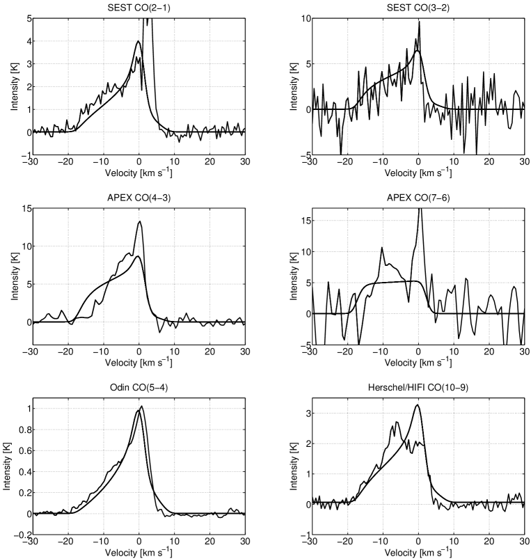
Figure 8: The six spectra obtained with SEST, APEX, Odin and Herschel compared to the best-fit model (see Sec. 4.3.1).

4.3.1 Density, temperature and water abundance

From the curved geometry model, the best fit gas density and kinetic gas temperature are $n$($\mathrm{H_{2}}$) = 9$\,\times\,10^{4}$ cm^-3 and $T_{\rm kin}$ = 180 K (formally 177 K) respectively. This implies a total H₂ mass of $\sim$1$\,\times\,10^{-2}$ $M_{\odot}$. The value of the reduced $\chi^{2}$ is 2.3. The CO spectra obtained with Odin, SEST and HIFI are plotted in Figure 8 together with the modelled spectra. The model fits the observations well, and we conclude that the geometry of the region can be a crucial parameter determining the shape of the line profiles. The CO (10$-$9) line observed with Herschel, however, shows a slightly more complicated profile than predicted (see discussion in Section 4.1). Thus, the triangular form is distorted by the presence of the $\upsilon_{\rm LSR}$ $\simeq-7$ $\mathrm{km\,s^{-1}}$ feature. A minor change in the kinetic temperature (i.e to 170 K) provides a better fit to the underlying triangular shape of the CO (10$-$9) line without affecting the lower-J CO lines by much. The computed maximum optical depths are $\leq$7$\,\times\,10^{-2}$ for all the modelled CO lines. Using the gas density and kinetic temperature obtained from the CO modelling, the observed o-H₂O ground state transition is best fit with an ortho-water abundance with respect to H₂ of $X(o$-$\mathrm{H_{2}O})$ = 1$\,\times\,10^{-5}$ (see Figure 11).

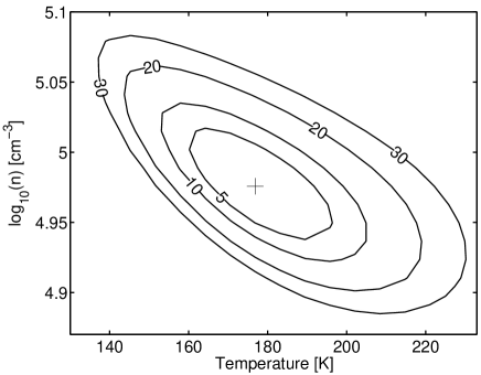
Figure 10: Contour plot showing the sum of the chi-squares, comparing the modelled spectra and the observations. The 5%, 10%, 20% and 30% deviations from the minimum value are indicated with solid lines. The best-fit density and temperature are indicated with a cross.

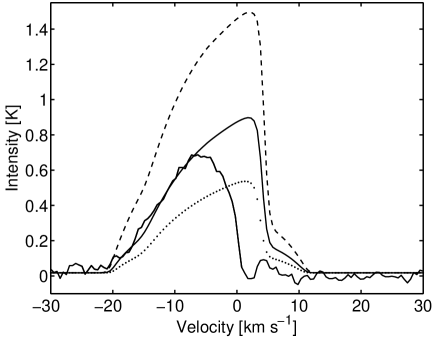
Figure 11: The HIFI $\rm{H_{2}O\,(1_{10}-1_{01})}$ spectrum compared with the model spectrum for $X(o$-$\mathrm{H_{2}O})$ = 1$\,\times\,10^{-5}$. Spectra with the o-H₂O abundance increased by a factor of two (dashed line) and decreased by a factor of two (dotted line) are also included included. Note that the foreground gas is visible in absorption in the observed spectrum.

The observed total flux in the map obtained with PACS corresponds to an integrated line intensity of 20 K $\mathrm{km\,s^{-1}}$. This is in agreement with the integrated intensity from the predicted line profile to within a factor of 2.

4.3.2 H₂O Line profile predictions

The line profiles for the six lowest rotational transitions of ortho-water have been computed. The abundance is set to 1$\,\times\,10^{-5}$ and the lines, that are predicted to be strong enough to be readily detected with HIFI, are displayed in Figure 12.

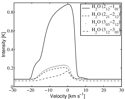
Figure 12: Line profile predictions for the $\rm{H_{2}O\,(2_{12}-1_{01})}$, $\rm{H_{2}O\,(2_{21}-2_{12})}$, $\rm{H_{2}O\,(3_{03}-2_{12})}$ and $\rm{H_{2}O\,(3_{12}-3_{03})}$ spectra as observed with HIFI.

Also in this figure, red-shifted emission originating from the opposite side of the sphere is present for the model with a curved geometry. Significant changes in the excitation temperature in the inner and outer shells show up in these spectra as weak absorption features. For this reason, the spectra have been computed using more than 100 shells to avoid any drastic changes in excitation temperature, due to optical depth effects between each shell. Simultaneously with the CO (10$-$9) observation, $\rm{H_{2}O\,(3_{12}-2_{21})}$ at 1153 GHz was also observed. The observed noise level of $\sim$0.1 K is however too high to detect the line with a predicted strength of only $\sim$10 mK. A summary of these predictions is presented in Table 4. In this table, the observed integrated intensity in the $\rm{H_{2}O\,(1_{10}-1_{01})}$ line is 30 % lower than the predicted value due to the absorption from foreground gas. If this gas is at a low temperature, however, the higher transitions should not be affected by much.

Table 4: The predicted integrated intensities, maximum intensities, continuum levels and optical depths for the six lowest rotational transitions of ortho-water. The maximum and integrated intensities are for the baselines subtracted spectra. The foreground absorption, visible in the observed $\rm{H_{2}O\,(1_{10}-1_{01})}$ spectrum, is not considered in this table.

Line	$\nu$	FWHM	Receiver	$\int{T}_{\mathrm{mb}}d\upsilon$	$10^{14}$ $\int{F}_{\lambda}d\lambda$	${T}_{\mathrm{mb},\mathrm{max}}$	$T_{\rm cont}$	$\tau_{\rm max}$
	(GHz)	(′′)		(K $\mathrm{km\,s^{-1}}$)	(erg cm-2 s-1)	(K)	(mK)
$\mathrm{1_{10}}$-$\mathrm{1_{01}}$	556.936	39	HIFI	12.9	9.3	0.88	18	40
$\mathrm{2_{12}}$-$\mathrm{1_{01}}$	1669.905	13	HIFI/PACS	13.0	28	0.80	80	44
$\mathrm{2_{21}}$-$\mathrm{1_{10}}$	2773.985	8	PACS	0.6	2.4	0.06	90	3.9
$\mathrm{2_{21}}$-$\mathrm{2_{12}}$	1661.017	13	HIFI/PACS	1.8	3.8	0.13	80	0.3
$\mathrm{3_{03}}$-$\mathrm{2_{12}}$	1716.775	13	HIFI/PACS	2.3	5.4	0.15	80	0.5
$\mathrm{3_{12}}$-$\mathrm{2_{21}}$	1153.117	19	HIFI	0.1	0.2	0.01	65	$<$0.1
$\mathrm{3_{12}}$-$\mathrm{3_{03}}$	1097.365	20	HIFI	1.0	1.4	0.10	62	$<$0.1
$\mathrm{3_{21}}$-$\mathrm{2_{12}}$	3977.047	5	PACS	0.3	1.3	0.02	103	0.3

4.3.3 Cooling rate ratios

For the curved model described in Sec. 4.3, we derive the cooling ratio $\Lambda({\rm CO})/\Lambda$(o-H₂O) $=10$ where the 557 GHz line is the dominant contributor to the water cooling. This value agrees well with the earlier determination of 7 based on ISO-LWS data and presented by Liseau et al. (1996).

4.3.4 The bump-like feature

As already discussed in Sec. 4.1, the bump-like feature seems unresolved to Herschel, i.e the size of the source is uncertain. A source size comparable to the beam size of Herschel, at 1152 GHz (19^′′), would have to have a high temperature ($>$1000 K) and low density ($\sim$10³ cm^-3) to fit the observations. This implies that the flux in the high-J CO lines would be higher than what was observed with ISO-LWS (Giannini et al., 2006). However, a source size as small as $\sim$1^′′, where the temperature and density would have to be $\sim$400 K and $\sim$10⁸ cm^-3 respectively, is a plausible scenario. In that case however, the ortho-water abundance has to be less than 10^-8 to fit with the ISO-LWS observations. In addition, the source is likely not smaller than 1^′′. Also in this case, the high-J CO lines would be stronger than what is actually observed.

Using a source size of 10^′′ (this size is estimated from H₂ maps presented in Neufeld et al. (2006)), the observed CO $"$bullet$"$-emission is well fit with a temperature, $T_{\rm kin}$ = 600 K, and a density, $n$($\mathrm{H_{2}}$) = 2$\,\times\,10^{4}$ cm^-3. This yields a column density, $N$($\mathrm{H_{2}}$) = 5$\,\times\,10^{20}$ cm^-2. For an ortho-water abundance of $X(o$-$\mathrm{H_{2}O})$ = 1$\,\times\,10^{-5}$, the $\rm{H_{2}O\,(3_{03}-2_{12})}$ emission is entirely accounted for by the ISO-LWS observations. In this case the $\rm{H_{2}O\,(2_{12}-1_{01})}$ emission would be merely about 25% of what was observed with PACS and no significant contribution would be observed in the $\rm{H_{2}O\,(1_{10}-1_{01})}$ line. Therefore, we conclude that the o-H₂O abundance in the $"$bullet$"$ is likely lower than 10^-5.

4.3.5 Comparison with other results

The derived H₂ density implies a column density of 5$\,\times\,10^{20}$ cm^-2 which is approximately one order of magnitude higher than what is derived for the warm gas (Neufeld et al., 2006). The best fit temperature, $T_{\rm kin}$ = 180 K, is significantly lower than the temperature in the gas responsible for the high-J CO emission [i.e CO (14$-$13) – CO (20$-$19)] reported in Giannini et al. (2006). Our model predicts these lines to be one to two orders of magnitude weaker. Clearly, different temperature regimes are present in HH 54 and a one-temperature, one-density model cannot explain all the infrared observations.

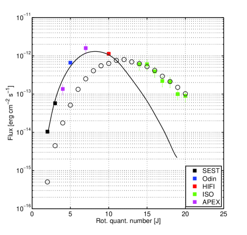
Figure 13: Observed CO line fluxes (squares) as a function of the rotational quantum number J. The errorbars are the estimated calibration uncertainties (10% for SEST, Odin and HIFI and 30% for APEX and ISO). The best fit model, described in the present paper (see Sec. 4.3.1), is indicated with a solid line. The fit to the high-J CO lines is indicated with black circles (see Sec. 4.3.5).

The high-J CO emission observed with ISO can be explained using the same geometry and source size but having a shell thickness 4$\,\times\,10^{14}$ cm, i.e one order of magnitude thinner. In that case a slightly higher density ($n$($\mathrm{H_{2}}$) = 1.5$\,\times\,10^{5}$ cm^-3) and temperature (T = 500 K) fits the high-J CO lines well. On the other hand, this secondary component also makes a significant contribution to the CO (10$-$9) line and this emission may originate from different components. Recently, Takami et al. (2010) report morphological differences between Spitzer observations in the 3.6, 4.5, 5.8 and 8.0 $\mu$m bands. The emission is observed to be less patchy in the long wavelength bands (i.e. 5.8 and 8.0 $\mu$m) and they interpret this as thermal H₂ emission being more enhanced in regions of lower density and temperature. Given the fact that hot gas obviously is present in this region, the secondary component may in reality be in smaller regions of high temperature similar to those observed in H₂. In Figure 13, the CO line flux is plotted as a function of the rotational quantum number, J.

The predicted integrated intensities can be compared with the modelling presented in Giannini et al. (2006). These authors present a multi-species analysis where they conclude that the observed H₂, CO and H₂O lines can only be explained by a J-shock with magnetic precursor. The C+J shock model, presented in their paper, explains the observed $\rm{H_{2}O\,(2_{12}-1_{01})}$ and $\rm{H_{2}O\,(3_{03}-2_{12})}$ line fluxes of 7$\,\times\,10^{-13}$ erg cm^-2 s^-1 and 2$\,\times\,10^{-13}$ erg cm^-2 s^-1 well, and they predict the line flux for the $\rm{H_{2}O\,(1_{10}-1_{01})}$ line to be 2.0 $\,\times\,10^{-13}$ erg cm^-2 s^-1. Converted to a K $\mathrm{km\,s^{-1}}$ scale these values correspond to 6.8, 1.4 and 53 K $\mathrm{km\,s^{-1}}$ respectively. Taking the beam size into account, the predicted integrated intensity for the $\rm{H_{2}O\,(1_{10}-1_{01})}$ line in this paper is at least a factor of four lower. This could be due to the fact that this line is very sensitive to the type of shock present. This is also discussed in the paper by Giannini et al. (2006), where they note that a J type shock would change the flux by more than a factor of two downwards.

Recently, Flower & Pineau des Forêts (2010) presented theoretical predictions of CO and H₂O line intensities, based on detailed C- and J-type shock model calculations. Expectedly, the assumed magnetic fields are different for their models of C- and J-shocks, i.e. for $b=1$ and $b=0.1$, respectively, where $b$ is defined through $B=b\sqrt{n_{\rm H}}\,\,\mu$G. For their high density C-shocks (see below), this means that pre-shock fields of order 450 $\mu$G should be present. Based on OH Zeeman observations, Troland & Crutcher (2008) detected 9 dark clouds in a sample of 34. Corresponding line-of-sight magnetic field strengths were in the range $B_{\rm los}=10-25\,\mu$G, with typical values around 15 $\mu$G. As discussed by Troland & Crutcher (2008), for randomly oriented fields, $B_{\rm los}=0.5\times\!\!\mid\!\!{\bf B}\!\!\mid$. Hence, magnetic fields in dark clouds do not likely exceed levels of $20-50\,\mu$G. This refers to the observed scales of 3^′. However, these authors also showed that in a given cloud, $B_{\rm los}$ did not change appreciably from one position (active molecular outflow) to another (quiescent surrounding cloud). It seems, therefore, that fields as strong as $450\,\mu$G may not be that common. On the other hand, order of magnitude lower field strengths ($45\,\mu$G for $b=0.1$) are more consistent with the observational evidence and may promote the occurrence of J-shocks.

For the radiative transfer Flower & Pineau des Forêts (2010) used an LVG approximation in slab geometry. In their Fig. 8, line profiles for CO (5-4) and $\rm{H_{2}O\,(1_{10}-1_{01})}$ are shown for C-shocks with two densities and four shock velocities. These lines are close in frequency and observations of HH 54 with Odin are made with essentially the same telescope beam, rendering resolution issues to be of only minor importance, i.e. any scaling of the intensities due to the source size should affect both observed lines in the same way. It should be feasible, therefore, to directly compare the line profiles of our Odin observations with those of the models by Flower & Pineau des Forêts (2010). Based on the observed maximum radial velocities, we consider only models with $\upsilon_{\rm s}\geq 20$ $\mathrm{km\,s^{-1}}$. Their models with shock velocities of 20 $\mathrm{km\,s^{-1}}$ could correspond to a head-on view, whereas their models for $\upsilon_{\rm s}$ = 30 and 40 $\mathrm{km\,s^{-1}}$ could correspond to inclinations of the flow with respect to the line of sight of 48^∘ and 60^∘, respectively.

For the C-shock models, several of the line profiles display shapes that are qualitatively similar to those observed with Odin and HIFI. These line shapes are a consequence of the computed flow variables, not a geometry effect. However, in particular for the range of $\Delta\upsilon\sim 0$ to about 10 km s^-1, the Odin/HIFI lines exhibit CO-to-H₂O intensity ratios very much in excess of unity, i.e. $T_{\rm CO}(\Delta\upsilon)/T_{\rm H_{2}O}(\Delta\upsilon)\gg 1$. $\Delta\upsilon$ is the velocity relative to the rest frame of the flow, i.e. $\upsilon_{\rm LSR}$.

These observed ratios are very much larger than the theoretical values (Fig. 14 and 15).

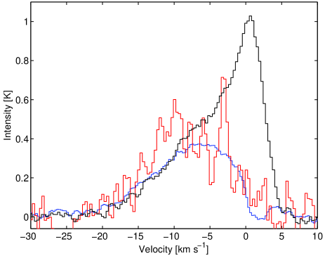
Figure 14: Comparison between the CO (5$-$4) line (black) and the $\rm{H_{2}O\,(1_{10}-1_{01})}$ line obtained with Odin (red). The H₂O spectrum has been multiplied with 6 for clarity. Also the HIFI $\rm{H_{2}O\,(1_{10}-1_{01})}$ spectrum has been plotted in this figure for comparison (blue). The intensity of the emission has in this case been multiplied by 6 and corrected for beam filling.

Albeit the ratios are larger than unity for the low-density ($n_{\rm H}=2\times 10^{4}$ cm^-3) C-shocks, these fall still far below the observed ones. On the other hand, the high density ($n_{\rm H}=2\times 10^{5}$ cm^-3) cases could directly be dismissed, as these tend to show inverted ratios, i.e. $T_{\rm CO}/T_{\rm H_{2}O}\,\ll 1$, contrary to what is observed (Fig. 15).

For the J-shock models, Flower & Pineau des Forêts (2010) list the predicted integrated intensities. Also in this case, the predicted CO-to-H₂O ratios (for a shock velocity of 20 $\mathrm{km\,s^{-1}}$) are much lower than the observed ratio, viz 0.06 and 0.005 for the pre-shock densities $n_{\rm H}=2\times 10^{4}$ cm^-3and $n_{\rm H}=2\times 10^{5}$ cm^-3 respectively.

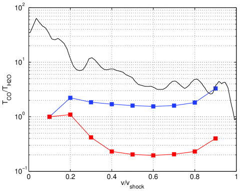
Figure 15: Line ratios between CO (5$-$4) and $\rm{H_{2}O\,(1_{10}-1_{01})}$. The ratio as measured from Odin is indicated with a black line. The predictions presented by Flower & Pineau des Forêts (2010) for $\upsilon_{\mathrm{shock}}$ =20 $\mathrm{km\,s^{-1}}$ are plotted in blue for $n$(H) = 2$\,\times\,10^{4}$ cm^-3 and in red for $n$(H) = 2$\,\times\,10^{5}$ cm^-3.

4.4 Implications for future work

The modelling of planar C-shocks show that low densities are required for cooling rate ratios, $\Lambda({\rm CO})/\Lambda$(o-H₂O) $>1$, in contrast to our own findings, where densities at least as high as 10⁵ cm^-3 seemed implied by the observations (Sect. 4.3.1). The cause for this mismatch is not clear to us, but one of the reasons could be the difference between modelled planar and curved geometry. Such modelling should therefore be attempted. The relatively high cooling rate ratio, $\Lambda({\rm CO})/\Lambda$(o-H₂O)$\leavevmode\nobreak\ =\leavevmode\nobreak\ 10$, is also not easily reconcilable with the presence of a C-type shock where a ratio, $\Lambda({\rm CO})/\Lambda$(o-H₂O) $\ll 1$ is favoured. On the other hand, J-shock models predict ratios even smaller than for C-shock models. However, the relatively low ortho-water abundance determined from the modeling indicate that J-type shocks may contribute.

As already discussed in Sect. 4.3.5, different temperature regimes are present in the HH 54 region. It would be adequate therefore, to repeat the ISO-LWS observations, using the higher sensitivity and spatial resolution provided by PACS. The mid-J CO lines fall in the wavelength range covered by the Spectral and Photometric Imaging Receiver (SPIRE) and these should be observed.

5 Conclusions

Based on spectral mapping with Herschel of the region containing the Herbig-Haro objects HH 52 to HH 54 we conclude the following:

• The CO ($10-9$) 1152 GHz line was clearly detected only toward the position of HH 54 with a FWHM $\stackrel{{\scriptstyle<}}{{{}_{\sim}}}$ 30^′′, comparable to the extent of the HH-emission knots in the visible and infrared.

• The $\rm{H_{2}O\,(2_{12}-1_{01})}$ 1669 GHz line was clearly detected toward HH 54 and with a similar extent as the CO ($10-9$) line. An offset of 9^′′ ($2.4\times 10^{16}$ cm) between the two species is observed, but the reality of this can at present not be firmly assessed. The $\rm{H_{2}O\,(1_{10}-1_{01})}$ 557 GHz line was also clearly detected toward HH 54.

• The CO ($10-9$) spectra show only blueshifted emission, with maximum relative velocities in excess of $-20$ $\mathrm{km\,s^{-1}}$. The line profiles exhibit typically a triangular shape, which in certain positions is however contaminated by a bump-like feature at $\upsilon_{\rm LSR}$ $=-7$ $\mathrm{km\,s^{-1}}$. This feature is constant in velocity and width. It is limited in spatial extent and may be identified by what is commonly called a $"$bullet$"$. Comparison of the observed spectra with analytical bow shock line profiles limits the viewing angle to greater than zero but $\stackrel{{\scriptstyle<}}{{{}_{\sim}}}$ 30^∘.

• The bump is clearly seen in position-velocity cuts, revealing two peaks, in addition to a smooth velocity gradient of about 10³ $\mathrm{km\,s^{-1}}$ pc^-1. The low-velocity peak appears close to the ambient cloud velocity, whereas the second peak corresponds to the bump. For this feature we determine from Gaussian fit measurement of the CO ($10-9$) data a relative peak-$T_{\rm mb}=1.5$ K, $\upsilon_{\rm LSR}$ $=-7$ $\mathrm{km\,s^{-1}}$ and FWHM = 5 $\mathrm{km\,s^{-1}}$.

• These line features are also observed in the CO ($5-4$) spectrum observed with Odin and in spectra obtained from the ground, i.e. in maps of the ($2-1$), ($3-2$), ($4-3$) and ($7-6$) CO transitions. In addition to the triangular line shape, these data do therefore also confirm the reality of the spectral bump.

• We initially use physical parameters for shock models of HH 54 found in the literature to compute the CO spectra. These models presented two-component fits, given by analytical expressions for temperature and density in the respective slabs. These models were only moderately successful in reproducing the observational results, in particular what regards the line shapes. Considerable improvement was found, however, in computed spectra using a curved geometry instead.

• Using the best fit model parameters (in a $\chi^{2}$-sense) for the CO data we computed spectra for H₂O. This model fits the H₂O 557 GHz line observed with HIFI for an ortho-water abundance with respect to molecular hydrogen, $X({\rm H_{2}O})=1\times 10^{-5}$.

• A cooling rate ratio, $\Lambda({\rm CO})/\Lambda$(o-H₂O) $\gg 1$, is not easily reconcilable with recent shock modelling. On the other hand, a relatively low water abundance ($\sim$$10^{-5}$), supports a scenario where J-shocks contribute significantly to the observed emission. This is also consistent with magnetic field strengths measurements toward dark clouds, where $B$-values lower than what is needed for C-type shocks, typically are observed.

• Comparison of our Odin data with line profiles from recent detailed C-shock model computations in the literature suggests that some refinements of these models may be required.

Appendix A

A.1 Extinction by dust and dust parameters

At the position of HH 54, the molecular cloud is relatively tenuous as the dust extinction through the cloud amounts merely to $A_{\rm V}$ $\sim$ 2-3 mag (Gregorio-Hetem et al. 1989; Cambrésy 1999). With the relations of Eqs (2) and (8) of Hayakawa et al. (2001), this results in a total H₂-column density of $N$($\mathrm{H_{2}}$)=$2\times 10^{21}$ cm^-2.

From [Fe II] line observations, Gredel (1994) determined the visual extinction toward the HH object as $A_{\rm V}$ = 1-3 mag, which could suggest that the blueshifted HH 54 is located at the rear side of the cloud, a circumstance that potentially explains the apparent absence of redshifted emission. However, an $R_{\rm V}$-value of $\stackrel{{\scriptstyle>}}{{{}_{\sim}}}$ 5, which is significantly higher than that used by Gredel (1994) and by others, needs to be invoked to describe the Cha II dust (see the discussion by Alcalá et al. 2008, and references therein). This reflects a predominantly ’big-grain’ contribution to the extinction (almost 2 magnitudes larger $A_{\rm V}$ per unit $E_{\rm B-V}$) and we consequently chose a shallower dust opacity dependence on the wavelength in the FIR and submm, identified by the parameter $\beta$ in Table 3, i.e. $\beta=1$ as opposed to $\beta=2$ for the general ISM For the normalisation wavelength used by Hildebrand (1983), i.e. $\lambda_{0}=250$ $\mu$m, we adopt the grain opacity $\kappa_{0}=25$ cm² g^-1 (Ossenkopf & Henning 1994). The corresponding mass absorption coefficient $\kappa$ at long wavelengths is then readily found from $\kappa_{\lambda}=\kappa_{0}(\lambda_{0}/\lambda)^{\beta}$.

Combining our own results with those found in the literature yields an SED of a putative core at 10 K which provides a strict upper limit to the luminosity. Any associated central point source would have a limiting luminosity of $L_{\rm bol}<0.4$ $L_{\odot}$. Assuming optically thin emission at long wavelengths and using standard techniques, the mass of the 10 K core/envelope is estimated at a mere 2 $M_{\oplus}$, excluding the possibility of a very young age of the hypothetical central source.

A.2 The exciting source

Several IRAS point sources are found in the surroundings of HH 54 and it is plausible to assume that one of these would be the exciting source of the HH object. Most often, the exciting source is a young ($\stackrel{{\scriptstyle<}}{{{}_{\sim}}}$ Myr) stellar object, situated at the geometrical centre of the bipolar outflow and this seems also to be the case for the CO outflow associable with IRAS $12515-7641$ near HH 52 and HH 53 (Knee 1992). For HH 54, the situation is different however: Knee (1992) identified IRAS $12522-7640$, which is positionally coincident with HH 54, as the driving source of a collimated blueshifted outflow. It seems however very unlikely that this IRAS source is (proto-)stellar in nature. It was detected essentially only, and barely, in the 60 $\mu$m-band, and it was shown that this IRAS flux is entirely attributable to [O i] 63 $\mu$m line emission (Liseau et al. 1996). More recent observations by Spitzer are in support of this conclusion, as these were unable to reveal any point source at this position (Alcalá et al. 2008).

On the basis of proper motion measurements and morphology considerations, Caratti o Garatti et al. (2009) proposed the Class I object IRAS $12500-7658$ to be the exciting source of HH 54. The IRAS source is located 20^′ south of HH 54, i.e. at the projected distance of 1 pc. It was not detected at 1200 $\mu$m by Young et al. (2005, see below). What regards HH 52 and HH 53, no satisfactory candidate was found by these authors. The possibility of different exciting sources was also considered by Nisini et al. (1996) and Alcalá et al. (2008), associating HH 52 and HH 53 with IRAS $12496-7650$ (DK Cha), whereas Ybarra & Lada (2009) identify this object also with the exciting source of HH 54.

In APEX-LABOCA maps at 870 $\mu$m, no emission was detected toward HH 54 nor from the Cha II cloud itself ($S_{870\mu{\rm m}}<20$ mJy beam^-1: van Kempen 2008). However, jet-like extensions are seen to emanate from both DK Cha and IRAS $12553-7651$ (ISO-Cha II 28), which are situated some 10^′ to 20^′ south/southeast of HH 54. Narrow, extended emission from these IRAS sources was also reported by Young et al. (2005), who used SEST-SIMBA to map the region at 1200 $\mu$m. The alignment with the HH objects is poor, however. Based on the observed spectral indices, this emission is dominated by optically thin radiation from dust. The dust features appear as tori or rings, seen edge-on, but given their sizes ($3\times 10^{4}$ AU), they do not represent what commonly is called a (protostellar) “disc”. Perhaps, these dust features are left-overs from an earlier history, during which the IRAS sources were formed. A “conventional disc” of size $\sim$ 10² AU could very well hide inside and any outflow would be orthogonal to these disc features.

Whereas the dust extension from DK Cha is not, whether direct or perpendicular, pointing anywhere near HH 52-54, the vector orthogonal to the linear feature of ISO-Cha II 28, at position angle 51^∘, is within 5^∘ from the current direction toward HH 54. Taking the uncertainty of this estimate into account, this coincidence appears very compelling. If this source drives/has driven a jet, that would very well be aligned with HH 54. The projected distance is 16^′ (0.8 pc), i.e. jet travel times would be of the order of $10^{4}\,(\upsilon/100\,{\rm km\,s}^{-1})^{-1}$ yr. With a total luminosity of $\sim$ 10 $L_{\odot}$ and a mass accretion rate of Ṁ${}_{\rm acc}=6\times 10^{-7}$ $M_{\odot}\,{\rm yr}^{-1}$ (Alcalá et al. 2008), ISO-Cha II 28 would make an excellent candidate for the exciting source of HH 54, the (distance corrected) stellar mass loss rate for which has been determined as Ṁ${}_{\rm loss}\leq 4\times 10^{-7}$ $M_{\odot}\,{\rm yr}^{-1}$ (Knee 1992), assuming a flow velocity of $\geq 100$ $\mathrm{km\,s^{-1}}$. A ratio of loss-to-accretion rate of $\leq 2/3$ would thus be indicated, a value which is in reasonable agreement with theoretical expectation for centrifugally driven MHD winds (Königl & Pudritz 2000; Shu et al. 2000; Contopoulos & Sauty 2001). To summarise, as also concluded by others before, the issue of the exciting source(s) of the HH objects 52, 53, 54 remains essentially unsettled.

Appendix B HIFI data reduction

The CO (10$-$9) data published in this paper are public to the scientific community and can be downloaded from the Herschel Science Archive (HSA). The two CO (10$-$9) observations were carried out in dual-beam-switch raster mode (observation id: 1342180798) and on-the-fly with position switch mode (observation id: 1342190901). The $\rm{H_{2}O\,(1_{10}-1_{01})}$ observation was carried out in point mode with position switch. The data reduction and production of the HIFI maps followed the following steps:

1. The raw data were imported to HIPE from the HSA.

2. All data were re-calibrated using v4.2 of the HIFI pipeline for CO (10$-$9) and v5.0 for $\rm{H_{2}O\,(1_{10}-1_{01})}$. There is a slight offset between the pointings for the horisontal and vertical polarisations. For that reason, separate readout positions were calculated for the two polarisations.

3. The level 2 data were exported to Class using the HiClass tool in HIPE.

4. A baseline was fitted to and subtracted from each individual spectrum. This step and the subsequent data reduction was carried out in xs.

5. From Figure 1, it is clear that the readout positions for the two CO (10$-$9) maps are not on a regular grid in RA and Dec. Instead of averaging nearby spectra together, a Gaussian weighting procedure was used. The FWHM of the two dimensional Gaussian used in the weighting was taken to be 9.3^′′. This size is larger than the average spacing between individual spectra but on the other hand small enough not to change the spatial resolution significantly.

6. In order to verify the quality of the CO (10$-$9) observations, spectra taken toward the same positions in the two different observing modes were compared, showing no significant differences. (see Figure 16). Also the horisontal and vertical polarisation data were reduced individually for both CO (10$-$9) and $\rm{H_{2}O\,(1_{10}-1_{01})}$ showing excellent agreement.

   

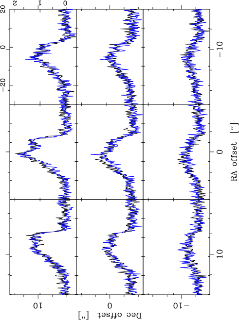
   Figure 16: CO (10$-$9) spectra toward HH 54. The black spectra are from the HIFI observation 1342180798, while the blue spectra are from the observation 1342190901. The horisontal and vertical polarisations have been averaged together (see text).

Appendix C Radiative transfer analysis

An Accelerated Lambda Iteration (ALI) method (e.g. Rybicki & Hummer 1991) is used to compute the line profiles for the observed transitions, varying only the density, kinetic temperature and the geometry of the shocked region. ALI is a method, where the coupled problem of radiative transfer and statistical equilibrium is solved exactly.

C.1 Accelerated Lambda Iteration

The ALI code has in recent years been used in several publications (see e.g Justtanont et al. 2005; Wirström et al. 2010) and was benchmarked with other codes in a paper by Maercker et al. (2008). In that paper, the ALI technique is described in more detail. In the present work, typically 30 shells and 16 angles are used. The statistical equilibrium equations and the equation of radiative transfer are solved iteratively until the relative level populations between each iteration changes by less than 10^-8. In the modelling we set the energy limit to 2000 K. 27 rotational energy levels, 26 radiative transitions and 351 collisional transitions are included in the calculations for CO. For o-H₂O, the corresponding numbers are 45, 164 and 990.

C.1.1 Collision rates

In recent years, substantial efforts have been made to determine cross-sections for H₂O excitation due to collisions with H₂. Quantal calculations governing collisions between H₂O and H₂ are to this date not complete and for o-H₂O, only collision rates for interaction with p-H₂ are available (Dubernet et al. 2009). For this reason we make the assumption that all p-H₂ are in the lowest energy state when solving the statistical equilibrium equations. It is also assumed that the p-H₂ stays in the ground state after the collision. The ortho-to-para ratio has been estimated for warm H₂ by Neufeld et al. (2006). These authors derive ratios significantly lower than 3, viz $\sim$0.4 - 2 in the HH 54 region. The computed spectra from the ALI modelling have also been compared with those, using the collision rates presented by Faure et al. (2007), and with similar results. In the case of CO, we use the collision rates presented by Yang et al. (2010).

References

- Alcalá et al. (2008) Alcalá, J. M., Spezzi, L., Chapman, N., et al. 2008, ApJ, 676, 427
- Bergin et al. (1998) Bergin, E. A., Neufeld, D. A., & Melnick, G. J. 1998, ApJ, 499, 777
- Bjerkeli et al. (2009) Bjerkeli, P., Liseau, R., Olberg, M., et al. 2009, A&A, 507, 1455
- Cambrésy (1999) Cambrésy, L. 1999, A&A, 345, 965
- Caratti o Garatti et al. (2009) Caratti o Garatti, A., Eislöffel, J., Froebrich, D., et al. 2009, A&A, 502, 579
- Caratti o Garatti et al. (2006) Caratti o Garatti, A., Giannini, T., Nisini, B., & Lorenzetti, D. 2006, A&A, 449, 1077
- Contopoulos & Sauty (2001) Contopoulos, I. & Sauty, C. 2001, A&A, 365, 165
- de Graauw et al. (2010) de Graauw, T., Helmich, F. P., Phillips, T. G., et al. 2010, A&A, 518, L6+
- Draine (1980) Draine, B. T. 1980, ApJ, 241, 1021
- Dubernet et al. (2009) Dubernet, M.-L., Daniel, F., Grosjean, A., & Lin, C. Y. 2009, A&A, 497, 911
- Faure et al. (2007) Faure, A., Crimier, N., Ceccarelli, C., et al. 2007, A&A, 472, 1029
- Flower & Pineau des Forêts (2010) Flower, D. R. & Pineau des Forêts, G. 2010, MNRAS, 406, 1745
- Franklin et al. (2008) Franklin, J., Snell, R. L., Kaufman, M. J., et al. 2008, ApJ, 674, 1015
- Giannini et al. (2006) Giannini, T., McCoey, C., Nisini, B., et al. 2006, A&A, 459, 821
- Gredel (1994) Gredel, R. 1994, A&A, 292, 580
- Gregorio-Hetem et al. (1989) Gregorio-Hetem, J. C., Sanzovo, G. C., & Lepine, J. R. D. 1989, A&AS, 79, 452
- Gusdorf et al. (2008) Gusdorf, A., Cabrit, S., Flower, D. R., & Pineau Des Forêts, G. 2008, A&A, 482, 809
- Güsten et al. (2006) Güsten, R., Nyman, L. Å., Schilke, P., et al. 2006, A&A, 454, L13
- Haro (1952) Haro, G. 1952, ApJ, 115, 572
- Haro (1953) Haro, G. 1953, ApJ, 117, 73
- Hartigan et al. (1987) Hartigan, P., Raymond, J., & Hartmann, L. 1987, ApJ, 316, 323
- Hayakawa et al. (2001) Hayakawa, T., Cambrésy, L., Onishi, T., Mizuno, A., & Fukui, Y. 2001, PASJ, 53, 1109
- Herbig (1950) Herbig, G. H. 1950, ApJ, 111, 11
- Herbig (1951) Herbig, G. H. 1951, ApJ, 113, 697
- Hildebrand (1983) Hildebrand, R. H. 1983, QJRAS, 24, 267
- Hjalmarson et al. (2003) Hjalmarson, Å., Frisk, U., Olberg, M., et al. 2003, A&A, 402, L39
- Hollenbach et al. (1989) Hollenbach, D. J., Chernoff, D. F., & McKee, C. F. 1989, in ESA Special Publication, Vol. 290, Infrared Spectroscopy in Astronomy, ed. E. Böhm-Vitense, 245–258
- Justtanont et al. (2005) Justtanont, K., Bergman, P., Larsson, B., et al. 2005, A&A, 439, 627
- Kaufman & Neufeld (1996) Kaufman, M. J. & Neufeld, D. A. 1996, ApJ, 456, 611
- Knee (1992) Knee, L. B. G. 1992, A&A, 259, 283
- Königl & Pudritz (2000) Königl, A. & Pudritz, R. E. 2000, Protostars and Planets IV, 759
- Lellouch et al. (2010) Lellouch, E., Hartogh, P., Feuchtgruber, H., et al. 2010, A&A, 518, L152+
- Liseau et al. (1996) Liseau, R., Ceccarelli, C., Larsson, B., et al. 1996, A&A, 315, L181
- Liseau & Sandell (1986) Liseau, R. & Sandell, G. 1986, ApJ, 304, 459
- Lovelace et al. (2010) Lovelace, R. V. E., Romanova, M. M., Ustyugova, G. V., & Koldoba, A. V. 2010, MNRAS, 408, 2083
- Maercker et al. (2008) Maercker, M., Schöier, F. L., Olofsson, H., Bergman, P., & Ramstedt, S. 2008, A&A, 479, 779
- Melnick et al. (2000) Melnick, G. J., Stauffer, J. R., Ashby, M. L. N., et al. 2000, ApJ, 539, L77
- Neufeld et al. (2006) Neufeld, D. A., Melnick, G. J., Sonnentrucker, P., et al. 2006, ApJ, 649, 816
- Nisini et al. (2007) Nisini, B., Codella, C., Giannini, T., et al. 2007, A&A, 462, 163
- Nisini et al. (1996) Nisini, B., Lorenzetti, D., Cohen, M., et al. 1996, A&A, 315, L321
- Nordh et al. (2003) Nordh, H. L., von Schéele, F., Frisk, U., et al. 2003, A&A, 402, L21
- Olberg (2010) Olberg, M. 2010, Technical Note: ICC/2010-nnn, v1.1, 2010-11-17
- Olberg et al. (2003) Olberg, M., Frisk, U., Lecacheux, A., et al. 2003, A&A, 402, L35
- Ossenkopf & Henning (1994) Ossenkopf, V. & Henning, T. 1994, A&A, 291, 943
- Ott (2010) Ott, S. 2010, in Astronomical Society of the Pacific Conference Series, Vol. 434, Astronomical Data Analysis Software and Systems XIX, ed. Y. Mizumoto, K.-I. Morita, & M. Ohishi, 139–+
- Pilbratt et al. (2010) Pilbratt, G. L., Riedinger, J. R., Passvogel, T., et al. 2010, A&A, 518, L1+
- Poglitsch et al. (2010) Poglitsch, A., Waelkens, C., Geis, N., et al. 2010, A&A, 518, L2+
- Rybicki & Hummer (1991) Rybicki, G. B. & Hummer, D. G. 1991, A&A, 245, 171
- Sandell et al. (1987) Sandell, G., Zealey, W. J., Williams, P. M., Taylor, K. N. R., & Storey, J. V. 1987, A&A, 182, 237
- Schwartz et al. (1984) Schwartz, R., Jones, B. F., & Sirk, M. 1984, AJ, 89, 1735
- Shu et al. (2000) Shu, F. H., Najita, J. R., Shang, H., & Li, Z. 2000, Protostars and Planets IV, 789
- Takami et al. (2010) Takami, M., Karr, J. L., Koh, H., Chen, H., & Lee, H. 2010, ApJ, 720, 155
- Troland & Crutcher (2008) Troland, T. H. & Crutcher, R. M. 2008, ApJ, 680, 457
- van Dishoeck et al. (2011) van Dishoeck, E. F., Kristensen, L. E., Benz, A. O., et al. 2011, PASP, 123, 138
- van Kempen (2008) van Kempen, T. 2008, PhD thesis, Leiden Observatory, Leiden University, P.O. Box 9513, 2300 RA Leiden, The Netherlands
- Whittet et al. (1997) Whittet, D. C. B., Prusti, T., Franco, G. A. P., et al. 1997, A&A, 327, 1194
- Wirström et al. (2010) Wirström, E. S., Bergman, P., Black, J. H., et al. 2010, A&A, 522, A19+
- Wu et al. (2004) Wu, Y., Wei, Y., Zhao, M., et al. 2004, A&A, 426, 503
- Yang et al. (2010) Yang, B., Stancil, P. C., Balakrishnan, N., & Forrey, R. C. 2010, ApJ, 718, 1062
- Ybarra & Lada (2009) Ybarra, J. E. & Lada, E. A. 2009, ApJ, 695, L120
- Young et al. (2005) Young, K. E., Harvey, P. M., Brooke, T. Y., et al. 2005, ApJ, 628, 283