Inter-shell exchange interaction in CdTe/ZnTe quantum dots: magneto-photoluminescence of X, X^2- and XX^-

Abstract

We present a comprehensive photoluminescence study of exchange interaction in self-assembled CdTe/ZnTe quantum dots. We exploit the presence of multiple charge states in the photoluminescence spectra of single quantum dots to analyze simultaneously fine structure of different excitonic transitions, including recombination of neutral exciton/biexciton, doubly charged negative exciton and negatively charged biexciton. We demonstrate that the fine structure results from electron-hole exchange interaction and that spin Hamiltonians with effective exchange constants $\delta_{i}$ can provide a good description of each transition in magnetic field for Faraday and Voigt field geometry. We determine and discuss values of the effective exchange constants for a large statistics of quantum dots.

I Introduction

Self-assembled quantum dots (QDs) are an ideal system when it comes to study physics of closely confined carriers. One of interesting aspects of such a system is the exchange interaction between the carriers. From a practical point of view, the electron-hole interaction in a single QD is described using two characteristic energies: an isotropic contribution responsible for bright-dark exciton splitting and anisotropic contribution related to fine structure splitting of bright states of a neutral exciton Gammon et al. (1996). The studies of exchange interaction in QDs attracted wide attention several years ago after the proposal of entangled photon generation in biexciton-exciton (XX-X) cascade Benson et al. (2000). The interest was focused mainly on reducing anisotropic part of the e-h exchange interaction, which hindered the entanglement between emitted photons. The research effort finally led to successful demonstration of fine structure control confirmed by observation of entanglement in XX-X cascadeStevenson et al. (2006); Akopian et al. (2006).

In our present work we describe the exchange interaction in CdTe/ZnTe QDs.

Such dots are very convenient for spectroscopy as they give strong photoluminescence (PL) in the visible range of the spectrum and exhibit well resolved excitonic lines. Another outstanding advantages of such dots is a feasibility of incorporation a localized $5/2$ spins by doping with manganese Besombes et al. (2004). A single Mn ion in a QD was shown to exhibit long ($t_{1}=0.4$ms) spin memory Goryca et al. (2009), which makes it an interesting candidate for quantum information storage. Precise knowledge of the exchange interaction in such QDs is of the essence due to its role in the optical orientation mechanism of the Mn spin Goryca et al. (2010). Our findings about electron-hole interaction in undoped self-assembled CdTe/ZnTe QDs should be also valid for Mn-doped dots.

Most of the studies on e-h exchange were devoted to interactions between $s$-shell carriers. Such an interaction is sufficient to describe a fine structure of neutral exciton (X), charged excitons (X⁺, X^-), and neutral biexciton (XX). On the other hand, the fine structure of doubly charged exciton (X^2-) and charged biexciton (XX^-) transitions is determined by an exchange interaction between a $p$-shell electron and an $s$-shell hole. It was shown that this interaction can be successfully described using the same approach as for the interaction between $s$-shell carriers, i.e., by introducing respective $p$-$s$ iso- and anisotropic exchange parameters as was demonstrated in Refs. Urbaszek et al., 2003; Akimov et al., 2005; Cade et al., 2006; Ediger et al., 2007. However, most of the previous reports discuss effects related either to X^2- or XX^- transitions. The simultaneous access to both complexes allows the cross-comparison of all related fine structures, which is an important test of the applicability limit of the used spin Hamiltonian model. To our knowledge, such a comparison was reported only for highly symmetric QDs with negligible anisotropic part of exchange interaction Urbaszek et al. (2003).

In this report, we present a comprehensive study of $s$-$s$ and $p$-$s$ electron-hole exchange interaction in CdTe/ZnTe QDs. The experiments involved a large ($>200$) number of single dots and therefore the results can be considered representative for the investigated system. In our study we focus particularly on transitions related to recombination of X^2- and XX^- excitons. We show that fine structures of these lines can be interpreted within a spin Hamiltonian featuring both iso- and anisotropic term of exchange interaction. For simplicity, we assume that single-particle orbitals are not affected by direct Coulomb interaction, which would be important for calculation of absolute transition energiesHawrylak (1999). Moreover, we test the applicability of our model by introducing a magnetic field either perpendicular (Faraday configuration) or parallel (Voigt configuration) to the QD plane. Finally, we compare the exchange parameters obtained independently from X, X^2-, and XX^- transitions to cross-check the consistency of our description.

II Samples and experimental setup

The samples were grown by molecular beam epitaxy (MBE) on GaAs substrate. The sample structure contained four layers deposited during the growth: a CdTe buffer (about 3$\mu$m), a ZnTe lower barrier (0.7 $\mu$m), a single CdTe QD plane, and a ZnTe capping layer (50-100 nm). The QDs were formed following the original idea of Tinjod et. al. Tinjod et al. (2003), in which a 2D CdTe layer is temporarily capped with amorphous tellurium to induce the transition to dots. A more detailed description of the sample growth can be found in Ref. Wojnar et al., 2008. Some of the samples were additionally post-processed by producing a gold shadow-masks with 200nm apertures. We did not find any significant differences in single dot properties between different samples apart from the distribution of the QD emission energies and the average charge state, which did not affect the results presented in this work.

The sample was cooled to temperatures 1.5–10K. Spatial resolution defined by the laser spot diameter was 0.5–2$\mu$m. The PL was excited non-resonantly, using an Ar-ion laser (cw, 514nm), a Nd:YAG laser (cw, 532nm) or a frequency doubled Ti:Sapphire femtosecond laser (pulsed, 400nm). The choice of the excitation laser affected only intensities (both absolute and relative) of the observed transitions and did not affect the energy spectrum, thus the excitation details were not relevant to the present work. The PL was analyzed using 0.3m - 0.5m spectrographs equipped with CCD cameras and/or avalanche photodiode detectors. A $\lambda/2$ waveplate in a motorized mount followed by a linear polarizer allowed us to perform repetitive automated measurements of polarization properties of QD emission.

Most of the zero-field results were obtained using continuous-flow cryostat with external microscope objective. The measurements exploiting magnetic field were performed in cryostat equipped with a split-coil superconducting magnet producing magnetic field up to 7T in Faraday or Voigt configuration. Single photon correlations were performed using Hanbury-Brown–Twiss detection scheme presented in detail in Ref. Suffczyński et al., 2006. A complementary magneto-PL experiment using stronger magnetic field up to 28T was performed in Grenoble High Magnetic Field Laboratory. In the latter case the measurement was not sensitive to the polarization of the PL signal.

III Typical single QD photoluminescence pattern

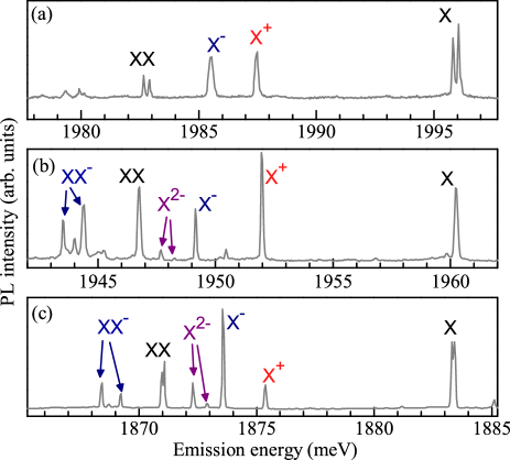
Figure 1: Three examples of typical emission pattern of a CdTe/ZnTe QD. Spectra were measured on different samples using non-resonant excitation (532nm or 400nm) at low temperature ($<2$K).

Studied dots were characterized by relatively large span of emission energies from about 1800 meV (nearly 700 nm) to 2250 meV (about 550 nm). A typical single dot spectra are shown in Fig. 1. Similar spectrum was observed by several groups Suffczyński et al. (2006); Léger et al. (2007); Lee et al. (2009), however only up to four strongest lines (X, X⁺, X^-, XX) were recognized. These lines tend to form a characteristic PL pattern with a single line separated from the others. This single line in the high-energy side of the PL spectrum is related to the neutral exciton, which can be confirmed e.g. by the anisotropy measurement (see Section IV). The next two lines in the spectrum are related to the charged excitons (X⁺, X^-). The signs of their charge state were distinguished basing on the charge tuning experiments on similar samplesLéger et al. (2006) and observation of negative optical orientation under quasi-resonant excitationKazimierczuk et al. (2009a). Such orientation was previously found for negatively charged excitons in different material systemsCortez et al. (2002); Dzhioev et al. (2002); Akimov et al. (2006). Finally, the last of the well established four lines is related to the recombination of neutral biexciton. It is evidenced by its polarization properties together with superlinear power dependence. Here we extend the description of the single dot spectrum by our experimental results used to identify X^2- and XX^- transitions. These transitions are closely related to $p$-$s$ electron-hole exchange interaction but were not identified previously in CdTe/ZnTe system.

We start with a discussion of relative energies (i.e. transition energies with respect to transition energy of neutral exciton) of these transitions in different dots. Such relative energies vary between dots with large random scatter on top of systematic changes with emission energy, as shown in Fig. 2(a). On average, the values of relative energy of XX transition in our dots are spread around 13.2 meV with standard deviation 1.3 meV (inset in Fig. 2(b)). We found that relative energies of various transitions for a single QD are strongly correlated. Data collected in Fig. 2(b) shows a clear linear dependence between relative energies of XX and charged excitons (X⁺, X^-, X^2-, and XX^-). This results in the same transition sequence for all dots but scattered energetic spread of the lines. Namely, the lines related to X^2- transition are present between X^- and XX lines in the typical PL spectrum while the ones related to XX^- transition are below XX line.

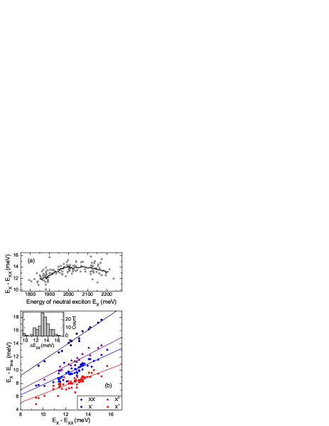
Figure 2: (a) Correlation of XX relative energy and absolute emission energy of X for different dots. A running average shown as a solid line is drawn to guide the eye. (b) Correlation of relative energies of various transitions for different dots. Solid lines mark linear ($y=ax$) fits with proportionality constants equal $a=0.64$ for X⁺, $a=0.78$ for X^-, $a=0.88$ for X^2-, and $a=1.15$ for XX^-. The inset presents distribution of XX relative energies.

A crucial point of our work is a correct identification of X^2- and XX^- transitions. A conclusive argument for XX^- identity was obtained by means of single photon correlation measurement. Such a measurement performed with pulsed excitation gives relative probability of the emission of two photons related to different transitions in a single excitation event. In particular, strong correlation peak is related to observation of two transitions from a single recombination cascade (such as $\left|\mathrm{XX}\right>\to\left|\mathrm{X}\right>\to\left|\emptyset\right>$). A histogram evidencing cascade recombination of XX^- and X^- complexes is shown in Fig. 3(a).

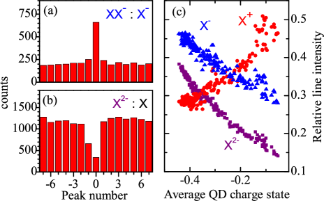
Figure 3: (a) Photon correlation histogram demonstrating XX^-–X^- emission cascade. (b) Anti-bunching cross-correlation between X^2- and X. Negative peak number corresponds to detection of X^2- after X. Both correlation experiments were done with pulsed ps excitation of 400nm with repetition 76MHz. (c) PL intensities of charged excitons relatively to the intensity of the neutral exciton. The estimate of the QD charge state is calculated as $\sum_{i}q_{i}I_{i}/\sum_{i}I_{i}$, where $I_{i}$ is the intensity of the transition related to charge state of $q_{i}$.

The photon cascade argument is not applicable to the case of X^2- transition. Single photon measurements between previously identified transitions and supposed X^2- transition show clear anti-bunchingKazimierczuk et al. (2010), which is expected for excitons of different charge states. Also the asymmetric shape of the histogram is characteristic for the correlation between charged and neutral excitons excited non-resonantlySuffczyński et al. (2006). The observed fine structure and magnetic field behavior (discussed further in Sections IV and V.1) indicated doubly charged exciton — X^2- or X²⁺. We determined the sign of the charge state by charge tuning experiment. We exploited here the fact that the average charge state of studied QDs depends on details of optical excitation, e.g., it can be modified by additional weak illumination with high-energy lightHaas et al. (2009). In the experiment, we measured intensities of all excitonic transitions while exciting a single QD simultaneously with two laser beams: 532nm and (much weaker) 400nm. By varying the intensity of 400nm laser beam we gradually changed the average charge state estimated as $\sum_{i}q_{i}I_{i}/\sum_{i}I_{i}$, where $I_{i}$ is an intensity of a transition related to charge state of $q_{i}$. The results of such an experiment were presented in Fig. 3(c). As expected X⁺ and X^- exhibit monotonic (increasing and decreasing respectively) dependence on the average QD charge state. Data for X^2- follows the behavior of X^-, which prove that these two complexes share the same sign of the charge state.

IV Fine structure

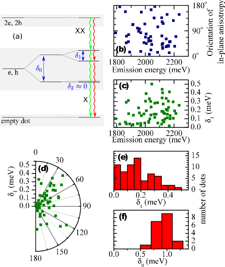
Figure 4: (a) A schematic energy diagram illustrating the fine structure of X and XX transitions. (b-d) Correlations between various parameters showing random character of in-plane anisotropy in CdTe/ZnTe dots: (b) orientation and (c) value of the anisotropic splitting of X transition versus emission energy and (d) value of anisotropic splitting and orientation of the in-plane anisotropy. (e) Histogram of the anisotropic splitting $\delta_{1}$ of X transition. (f) Histogram of bright–dark exciton splitting $\delta_{0}$.

Polarization resolved photoluminescence measurements represent an important and very time-effective characterization tool. In general, polarization dependence of the QD emission spectrum is related to in-plane anisotropy of the confining potential. Possible physical origins of this anisotropy include non-cylindrical symmetry of the QD shape, in-plane strain or electric field or the symmetry of the interfaces between barriers and the QDKudelski et al. (2001). The in-plane anisotropy was thoroughly studied for many years because of its destructive role in the scheme of entangled photon pair generation Benson et al. (2000). It was shown that a satisfactory description of the anisotropy-induced exciton splitting can be achieved by introducing an anisotropy of exchange interaction between electron and heavy hole. This interaction can be parametrized by three quantities:

$$2\langle\downarrow\Uparrow\mid H_{\mathrm{exch}}\mid\downarrow\Uparrow\rangle=-2\langle\downarrow\Downarrow\mid H_{\mathrm{exch}}\mid\downarrow\Downarrow\rangle = \delta_{0}$$ (1)

$$2\langle\downarrow\Uparrow\mid H_{\mathrm{exch}}\mid\uparrow\Downarrow\rangle = \delta_{1}$$ (2)

$$2\langle\downarrow\Downarrow\mid H_{\mathrm{exch}}\mid\uparrow\Uparrow\rangle = \delta_{2}$$ (3)

where $H_{\mathrm{exch}}$ is the effective exchange interaction and $\downarrow$ and $\Downarrow$ represent z-component spin projection of the electron and the hole respectively Bayer et al. (2002). These parameters are usually related to the fine structure of a neutral exciton (Fig. 4(a)): splitting between dark and bright branch ($\delta_{0}$), splitting between two bright configurations ($\delta_{1}$), and splitting between two dark excitons ($\delta_{2}$). In the present work we neglect the presence of dark exciton splitting (i.e., $\delta_{2}=0$). This assumption is justified by very small values of $\delta_{2}$ (of order of a few $\mu$eV Poem et al. (2010)), never resolved in our experiments.

We performed systematic measurements of PL polarization properties to determine the influence of the in-plane anisotropy on the typical emission pattern of single QDs in our samples. In the experiment we recorded the PL spectra for a number of linear polarization directions for each studied dot. Such a procedure was necessary due to a large scatter of the anisotropy axis between different QDs, usually observed in II-VI systems Kudelski et al. (2000). The collected data allowed us to determine actual principal axis of each QD and analyze the corresponding PL spectra. For dots with small anisotropic splitting (smaller than our experimental resolution), we determined the value of the splitting by fitting a gaussian profile to the whole collected dataset as described in Ref. Kowalik et al., 2007.

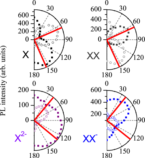
Figure 5: Polar plots presenting orientation of anisotropy-related linear polarization of various lines in the spectrum of a typical single QD. Empty symbols are related to the higher-energy component of each transition.

We start our discussion with analysis of the spectral lines related to the recombination of the neutral excitonic complexes: X and XX. In the former case, the zero-field emission consist of two closely spaced lines related to spin configurations build from $\uparrow\Downarrow$ and $\downarrow\Uparrow$ statesBayer et al. (2002). These two lines are separated by the energy $\delta_{1}$ and are visible in two perpendicular linear polarizations. The same underlying splitting of neutral exciton state affects also XX transition which also features polarization-resolved doublet split by $\delta_{1}$. Different ordering of the components of XX and X transitions results from different role of neutral exciton state in both cases: as final and initial state of the transition respectively. Figure 4(b-d) shows correlations of various anisotropy-related parameters for a set of measured dots. Coherently with previous reports on the anisotropy in a similar system Kudelski et al. (2000), we observe no preferential direction of the in-plane anisotropy. Neither the splitting value nor the anisotropy direction exhibit significant correlation with the transition energy or the biexciton relative energy.

Single charged excitons (X⁺, X^-) do not exhibit noticeable fingerprints of in-plane anisotropy. This is expected since the electron-hole exchange interaction influences neither the initial (where two majority carriers are forming closed shell with $S=0$) nor the final state (only one carrier left) of the transition. Although some degree of linear polarization of charged exciton transitions may arise due to valence band mixing Léger et al. (2007), we did not concentrate on this effect in our study due to its negligible intensity in the studied samples.

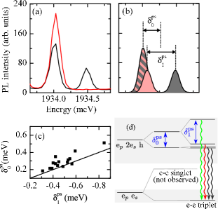
Figure 6: (color online) (a) Typical photoluminescence signature of X^2- recombination in investigated dots. Black and red (gray) curves correspond to two orthogonal linear polarizations. (b) Structure of the X^2- emission spectrum. Curve fill denotes line polarization (plain fill corresponds to full linear polarization, striped pattern corresponds to unpolarized line). (c) A set of X^2- exchange parameters for 15 different dots. The line corresponds to relation $2\delta_{0}^{ps}=-\delta_{1}^{ps}$. (d) A schematic illustration of the X^2- fine structure in analogy to the structure of the neutral exciton shown in Fig. 4(a). The final state in the figure corresponds to the spin triplet configuration.

The remaining two transitions — X^2- and XX^- — exhibit more complex fine structure Kazimierczuk et al. (2009b). Interestingly, we observed that the orientation of the linear polarization of X^2- and XX^- lines can be different than the orientation of the linear polarization of X and XX lines (Fig. 5). The mismatch between these orientation is relatively small and varies from dot to dot. Nevertheless, this difference clearly indicates a presence of additional anisotropic interaction in X^2- and XX^- complexes. We identify it as an exchange interaction between a hole and $p$-shell electron.

In further considerations we tentatively assume that the in-plane anisotropy significantly lifts the degeneracy between $p_{x}$ and $p_{y}$ orbitals. We also assume that the non-radiative relaxation of the excitonic complex with an electron at the higher-energy orbital is much faster than its optical recombination. In other words, we interpret the splitting patterns taking into account only single excited ($p$-shell) level without any contribution from orbital angular momentum. The spin part of the wavefunction is sufficient to describe all observed effects.

Recombination of X^2- was previously studied in GaAs-based dots by several groups with results qualitatively different in terms of light polarization Ediger et al. (2007); Urbaszek et al. (2003); Poem et al. (2007). In our samples, we found that the X^2- transition consists mainly of two emission lines separated by approximately $0.5$meV as shown in Fig. 6(a). The higher-energy line is significantly (5$\times$) weaker than the lower-energy one and is completely linearly polarized, similarly to the case described in Ref. Ediger et al., 2007. The lower energy line exhibits a partial linear polarization in the orthogonal direction. This splitting pattern arises from the electron-hole exchange interaction in the initial state of the transition. In the initial state, only two out of three electrons can accommodate in the lowest s orbital forming a closed shell. The remaining electron on the ${p}$ shell interacts with the hole, similarly to the interaction between carriers forming a neutral exciton. This analogy allows us to understand the arising splitting pattern, however one has to note differences in the exchange energies (denoted by $\delta_{0}^{ps}$ and $\delta_{1}^{ps}$ for isotropic and anisotropic part respectively) and selection rules (each state of X^2- is bright).

The final state of the considered transition consists of two electrons which form either spin singlet or triplet configuration, typically separated by several meVFinley et al. (2001). The optical transitions involve recombination of an electron and a hole of opposite spin orientations, therefore the “dark” configurations ($\left|{{\uparrow}\atop{\uparrow\downarrow}}\Uparrow\right>$, $\left|{{\downarrow}\atop{\uparrow\downarrow}}\Downarrow\right>$) recombine to the triplet states ($\left|{{\uparrow}\atop{\uparrow}}\right>$, $\left|{{\downarrow}\atop{\downarrow}}\right>$). The “bright” states can recombine either to singlet or triplet state. Therefore, for the spin singlet final state we expect only a pair of lines of equal intensity in the PL spectrum. Experimentally measured spectrum is more complex, thus we suppose that the observed transitions are related to the triplet configuration in the final state. Indeed, in such a case, one expect three emission lines (Fig. 6(d)): unpolarized emission from the “dark” state and two linearly polarized lines from anisotropy-split “bright” doublet. One should note that “bright”/“dark” labels are used here only in analogy to the case of neutral exciton. Actual intensity of “dark” exciton recombination is two times stronger than “bright” exciton recombination in case of X^2-, as the oscillator strength of the “bright” state recombination is divided into spin singlet and triplet configurations of the final state.

A typical PL spectrum of X^2- and corresponding decomposition into elementary transitions discussed above are presented in Figs. 6(a-b). Experimental data indicate a close coincidence of energies of the unpolarized line and lower component of the anisotropy-split doublet. Such a coincidence can be expressed in terms of exchange parameters as a relation: $2\left|\delta_{0}^{ps}\right|\approx\left|\delta_{1}^{ps}\right|$. This property was observed for all our dots for which X^2- transition was seen. Surprisingly, a similar coincidence was observed also for anisotropic InAs/GaAs QD Ediger et al. (2007). No underlying reason for this coincidence has been proposed so far.

In order to analyze quantitatively the relation between $\delta_{0}^{ps}$ and $\delta_{1}^{ps}$ we performed simultaneous fitting of spectra in both polarizations. This procedure allowed us to separate isotropic and anisotropic contributions to the exchange interaction. The results of the fitting procedure are presented in Fig. 6(c). By averaging the extracted values we established typical values of exchange parameters as $\delta_{0}^{ps}=\left(0.29\pm 0.08\right)$ meV and $\delta_{1}^{ps}=\left(-0.49\pm 0.12\right)$ meV.

Negative sign of $\delta_{1}^{ps}$ is related to the fact, that the $\frac{1}{\sqrt{2}}\left(\left|{{\uparrow}\atop{\uparrow\downarrow}}\Downarrow\right>+\left|{{\downarrow}\atop{\uparrow\downarrow}}\Uparrow\right>\right)$ state has lower energy than $\frac{1}{\sqrt{2}}\left(\left|{{\uparrow}\atop{\uparrow\downarrow}}\Downarrow\right>-\left|{{\downarrow}\atop{\uparrow\downarrow}}\Uparrow\right>\right)$ state, while in the case of the neutral exciton $\frac{1}{\sqrt{2}}\left(\left|{{}\atop{\uparrow}}\Downarrow\right>+\left|{{}\atop{\downarrow}}\Uparrow\right>\right)$ state has higher energy than $\frac{1}{\sqrt{2}}\left(\left|{{}\atop{\uparrow}}\Downarrow\right>-\left|{{}\atop{\downarrow}}\Uparrow\right>\right)$ state. However, one has to take into account the difference in the selection rules for X and X^2-. Namely, the lines related to recombination of $\frac{1}{\sqrt{2}}\left(\left|{{\uparrow}\atop{\uparrow\downarrow}}\Downarrow\right>+\left|{{\downarrow}\atop{\uparrow\downarrow}}\Uparrow\right>\right)$ and $\frac{1}{\sqrt{2}}\left(\left|{{}\atop{\uparrow}}\Downarrow\right>+\left|{{}\atop{\downarrow}}\Uparrow\right>\right)$ states have two opposite linear polarizations. This difference arises due to the fermionic nature of the electronsPoem et al. (2007) and is related to the sign of the $P_{\pm}$ matrices given in the Appendix A. Therefore, in spite of negative value of $\delta_{1}^{ps}$, the linearly polarized emission lines of X and X^2- exhibit the same order in the PL spectrum.

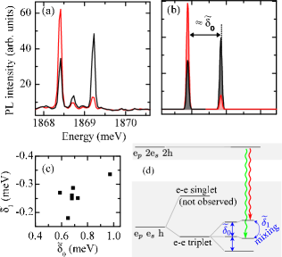
Figure 7: (color online) (a) Typical PL signature of XX^- recombination. Black and red (gray) curves correspond to two orthogonal linear polarizations. (b) Simulated XX^- emission spectrum. Curve fill denotes polarization (c) Correlation between two figures of merit for XX^-: $\widetilde{\delta_{1}}$ and $\widetilde{\delta_{0}}$. The presented data were obtained by fitting field dependence as discussed in Section V.2. (d) Schematic energy diagram illustrating the origin of XX^- fine structure

We studied the role of the p-shell electron also in the fine structure of the XX^- transition. The typical spectrum of XX^- transition is presented in Fig. 7(a). It consist of two lines. The intensity ratio of these lines is close to 2:1 in favor of the lower energy line. Both lines exhibit partial linear polarization. In this case the fine structure is determined mainly by the final state. In the initial state (3 electrons + 2 holes) the electron-hole exchange interaction is cancelled by paired hole spins. Similarly to the previously discussed X^2- transition, spectroscopic signature of XX^- transition fits to the case of triplet configuration of electrons remaining in the final state (see Fig. 7(d)). Its degeneracy is lifted by the exchange interaction with remaining hole forming three nearly-equidistant levels. In the simple picture of a symmetric dot, the splittings should be equal to $\widetilde{\delta}_{0}=\frac{1}{2}\left(\delta_{0}+\delta_{0}^{ps}\right)$ as they result from the interaction between both $s$ and $p$ electron with the hole. Only two out of three (four out of six including Krammers degeneracy) configurations of the final state are optically active, giving rise to two emission lines of XX^- transition in the PL spectrum. The forbidden configurations correspond to parallel spin orientations of all confined carriers ( $\left|{{\uparrow}\atop{\uparrow}}\Uparrow\right>$ and $\left|{{\downarrow}\atop{\downarrow}}\Downarrow\right>$).

The in-plane anisotropy manifests itself as mixing of the abovementioned states by off-diagonal element proportional to $\widetilde{\delta}_{1}=\frac{1}{2}\left(\delta_{1}+\delta_{1}^{ps}\right)$. In general, this addition should account for (possible) misorientation between anisotropy of s and p shells, however in most cases the experimentally determined mismatch between the two orientations is small. The strength of this mixing can be evaluated by measuring the degree of linear polarization of the corresponding PL lines. By diagonalization of a Hamiltonian including both isotropic and anisotropic part of the exchange interaction we found that the splitting between two components of XX^- transition is given by $\sqrt{\widetilde{\delta}_{0}^{2}+\frac{1}{2}\widetilde{\delta}_{1}^{2}}$. Linear polarization degree ($P=\frac{I_{\perp}-I_{||}}{I_{\perp}+I_{||}}$) of both lines is given by:

$$P=\frac{4\beta}{1\pm 3\sqrt{1+2\beta^{2}}}$$ (4)

where $\beta=\widetilde{\delta}_{1}/\widetilde{\delta}_{0}$ and sign ‘$+$’ corresponds to the stronger of the two lines (i.e. line corresponding to $\left|{{\uparrow}\atop{\uparrow}}\Downarrow\right>$ and $\left|{{\downarrow}\atop{\downarrow}}\Uparrow\right>$ configurations in case of a symmetrical dot).

The presented relations enable us to determine $\widetilde{\delta}_{0}$ and $\widetilde{\delta}_{1}$ values separately. We found that in our dots the average values of the exchange parameters were: $\widetilde{\delta}_{0}=\left(0.75\pm 0.16\right)$ meV and $\widetilde{\delta}_{1}=\left(-0.28\pm 0.08\right)$ meV. Within a spin Hamiltonian picture used here, these values can be independently obtained by measuring separately electron-hole exchange parameters for $s$- and $p$-shell electron. Using previously determined $\delta_{i}$ and $\delta_{i}^{ps}$ values we found:

$$\widetilde{\delta}_{0}^{\mathrm{(calc)}} = \frac{1}{2}\left(\delta_{0}+\delta_{0}^{\mathrm{ps}}\right)=\left(0.60\pm 0.08\right)\mathrm{\ meV}$$ (5)

$$\widetilde{\delta}_{1}^{\mathrm{(calc)}} = \frac{1}{2}\left(\delta_{1}+\delta_{1}^{\mathrm{ps}}\right)=\left(-0.16\pm 0.09\right)\mathrm{\ meV}$$ (6)

The values determined by combining the X and X^2- fine structure parameters are close to the values obtained from analysis of XX^- emission. A small but not negligible difference between them gives a measure of applicability of spin Hamiltonian approach to the fine structure of the studied transitions.

V Magnetophotoluminescence

Our study was completed by PL measurements in the magnetic field. The experiment was performed for two field configurations — in-plane (Voigt configuration) or along the growth axis (Faraday configuration). In both cases, the influence of the magnetic field can be well described by linear Zeeman term related to the spin and quadratic diamagnetic shift related to the extension of the exciton wavefunction. In the present work we were interested mainly in the influence of the magnetic field through the Zeeman term on the fine structure of the excitonic states.

The magnitude of the magnetic interaction is governed by values of electron and hole g-factors. For simplicity, in further considerations we abstract from valence band effects and introduce $\frac{1}{2}$ pseudospin for the $s$-shell hole with effective anisotropic g-factor encapsulating e.g. heavy-light hole mixing. In this convention the Zeeman splitting of the neutral exciton in Faraday configuration is given by $\left(g_{h}^{\mathbf{z}}-g_{e}^{\mathbf{z}}\right)\mu_{\mathrm{B}}B$. For the same purpose, we assume that $s$- and $p$-shell electrons are characterized by the same g-factor. We also assume no contribution of the orbital angular momentum of $p$-shell electron, possibly due to anisotropy-related degeneracy lifting of two $p$ orbitals.

V.1 Magnetophotoluminescence of X^2-

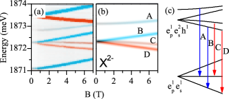
Figure 8: (color online) (a) Experimental and (b) simulated PL spectrum of X^2- in magnetic field in Faraday configuration. Color saturation denotes degree of circular polarization (blue — $\sigma+$, red — $\sigma-$) and brightness denotes the PL intensity. (c) Schematic of the corresponding energy diagram.

We start the discussion with the case of X^2- transition in the Faraday configuration. A typical data obtained in such an experiment is shown in Fig. 8(a). The magnetic field splits the lower energy component of X^2- transition into three lines (denoted B, C, D in Fig. 8(b)). The higher energy component (denoted A) does not split. All four lines are naturally organised in two pairs, each consisting of $\sigma+$ and $\sigma-$ polarized (fully or partially) components of equal intensities. The stronger pair (B and D) is characterized by splitting linear with field and it originates from the lower energy component at $B=0$. Conversely, the other pair (A and C) is already split at $B=0$ and the magnetic field induces only small increase of the splitting.

The observed behavior can be analyzed in analogy to neutral exciton, invoked in the previous Section. In such a picture, the two pairs of lines correspond to the two branches of the initial state: “bright states” and “dark states”. The magnetic field acts on each branch independly. The splitting of each branch is increasing according to $\sqrt{\delta^{2}+\left(g\mu_{\mathrm{B}}B\right)^{2}}$ where $\delta$ corresponds to splitting at $B=0$ and $g$ is a respective excitonic Landè factor. In such approach, the main difference between the two branches is their zero-field splitting. Perfectly linear splitting of the “dark branch” originates from negligible $\delta_{2}^{ps}$ value while substantial zero-field splitting of the “bright branch” ($\delta_{1}^{ps}$) dominates over the field-dependent contribution in the latter case.

The presented analogy is instructive, however it is not perfect. Particularly, it ignores the structure of the final state which is also affected by the magnetic field. It is important especially for recombination of “dark states”, which according to selection rules lead to $S=\pm 1$ branches of the final triplet state (Fig. 8(c)). As a result, the optically observed splitting of a “dark states” is governed by the same excitonic Landè factor as the “bright states” (i.e., $g_{e}^{\mathbf{z}}-g_{h}^{\mathbf{z}}$) and not the Landè factor of the real dark neutral exciton (i.e., $g_{e}^{\mathbf{z}}+g_{h}^{\mathbf{z}}$). This effect can be also seen as a result of the fact that the unpaired electron from the initial state is not the same electron that is recombining with the hole.

Transition	Field dependence ($B||z$) from the spin Hamiltonian
X	$\frac{1}{2}\left(\delta_{0}\pm\sqrt{\delta_{1}^{2}+\left(\left(g_{e}^{\mathbf{z}}-g_{h}^{\mathbf{z}}\right)\mu_{\mathrm{B}}B\right)^{2}}\right)$
X+ and X-	$\pm\left(g_{e}^{\mathbf{z}}-g_{h}^{\mathbf{z}}\right)\mu_{\mathrm{B}}B$
X2-	$\frac{1}{2}\left(\delta_{0}^{ps}\pm\sqrt{\left(\delta_{1}^{ps}\right)^{2}+\left(\left(g_{e}^{\mathbf{z}}-g_{h}^{\mathbf{z}}\right)\mu_{\mathrm{B}}B\right)^{2}}\right)$
	$\frac{1}{2}\left(-\delta_{0}^{ps}\pm\left(g_{e}^{\mathbf{z}}-g_{h}^{\mathbf{z}}\right)\mu_{\mathrm{B}}B\right)$
XX-	$\frac{1}{2}\left(-\widetilde{\delta}_{0}+\sqrt{2\widetilde{\delta}_{1}^{2}+\left(\widetilde{\delta}_{0}\pm(g_{e}^{\mathbf{z}}-g_{h}^{\mathbf{z}})\mu_{B}B\right)^{2}}\right)$
	$\frac{1}{2}\left(-\widetilde{\delta}_{0}-\sqrt{2\widetilde{\delta}_{1}^{2}+\left(\widetilde{\delta}_{0}\pm(g_{e}^{\mathbf{z}}-g_{h}^{\mathbf{z}})\mu_{B}B\right)^{2}}\right)$

Table 1: Field dependence of transition energies in Faraday configuration obtained from the spin Hamiltonian (neglecting diamagnetic shift).

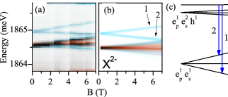
Figure 9: (color online) (a) Experimental and (b) simulated PL spectrum of X^2- in magnetic field in Voigt configuration. Color saturation denotes degree of linear polarization (red — $\vec{E}\parallel\vec{B}_{\mathrm{ext}}$, blue — $\vec{E}\perp\vec{B}_{\mathrm{ext}}$) and brightness denotes the PL intensity. A mismatch between orientation of magnetic field and the QD anisotropy was $16^{\circ}$. (c) Schematic of the corresponding energy diagram. Transitions related to characteristic splitting of higher-energy component were marked with arrows.

PL measurements in Voigt configuration revealed qualitatively different behavior of X^2- transition (Fig. 9(a)). This was confirmed by repetition of the measurements for a number of dots with different relative orientations of the in-plane anisotropy axis and the magnetic field. In each case we observed splitting of the higher-energy component into two lines and difficult to resolve multiple splitting of lower-energy component.

This spectral features are completely reproduced by the model based on spin Hamiltonian given in Appendix A as shown in Fig. 9(b). The simulations confirm that the double splitting of the higher-energy component does not depend on the relative orientation of in-plane anisotropy. On the other hand, such a dependence was found in the spectral lines split from the lower-energy component. Detailed analysis of the involved energy levels allowed us to conclude that the two characteristic lines split from the higher-energy component are transitions from the same initial state to $S_{\mathrm{x}}=\pm 1$ states of the final triplet configuration (Fig. 9(c)). Thus, this splitting is a clear measure of a (doubled) in-plane g-factor of an electron. Using this measure we found an average value of the electron in-plane g-factor $g_{e}^{\mathbf{x}}=0.62$.

V.2 Magnetophotoluminescence of XX^-

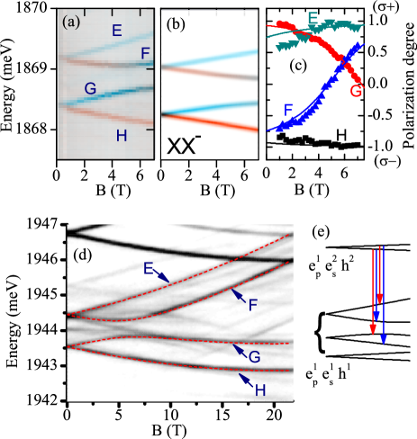
Figure 10: (color online) (a) Magnetophotoluminescence of XX^- transition in Faraday configuration (field along the growth axis). Blue and red represents $\sigma+$ and $\sigma-$ polarization respectively. (b) Result of simulation using spin Hamiltonian given in Appendix A. (c) Degree of circular polarization for different components of XX^- as a function of magnetic field for the same QD. (d) Magnetophotoluminescence of XX^- transition for a different dot measured in a resistive magnet (no polarization resolution). Fitted model is shown by dashed lines. (e) Schematic of QD energy levels.

As it was shown in Section IV, the zero field spectral signature of XX^- consists of two emission lines. Figure 10(a) presents an evolution of this structure with external magnetic field in the Faraday configuration. Initially, for field up to a few tesla, both lines exhibit typical Zeeman splitting into two circularly polarized components. However, the linearity of the Zeeman effect is perturbed in the stronger field and an anticrossing between two inner spin-split components is observed. The anticrossing is accompanied by characteristic exchange of line polarization, depicted in Fig. 10(c).

The observed anticrossing is precisely reproduced by the model based on the spin Hamiltonian (Fig. 10(b)). Similarly to the fine structure at $B=0$, the field dependence is governed mainly by the final states of the transitions. The anticrossing is due to the off-diagonal anisotropic part of the e-h exchange interaction ($\widetilde{\delta}_{1}$). The model calculation reproduce also quantitatively the measured polarization behavior (Fig. 10(c)). It is worth to note that for none of the spectral lines the field corresponding to complete linear polarization (and thus zero circular polarization) coincides with the actual anticrossing point determined as a point of minimum energy separation between the lines. Instead, at the anticrossing point both involved lines exhibit elliptical polarization with the same contribution of $\sigma+$ polarization. Such an effect is not related to the properties of the anticrossing states, but rather to the difference in the values of transition matrix elements (see Appendix A).

The field dependence of XX^- transition energies and particularly the anticrossing strength is a direct measure of $\widetilde{\delta}_{1}$. We verified that indeed the same pair of $\widetilde{\delta}_{i}$ values fits transition energies and corresponding polarization degrees with and without magnetic field. For example, the magnetic field measurements on a dot in Fig. 10(a,c) allowed us to obtain $\widetilde{\delta}_{0}=0.69$ meV and $\widetilde{\delta}_{1}=-0.29$ meV. By substituting these values to Eq. 4 we predict degree of zero field linear polarization for both PL lines of this particular dot as $0.37$ and $-0.68$, while in the independent measurement we found them to be equal to $0.36$ and $-0.69$.

Experiments in high magnetic field allowed us to compare the model predictions with data measured in a wide range of applied field. Figure 10(d) show example of the PL obtained in a scan up to 22T. The data clearly show the previously discussed anticrossing between two bright transitions. In principle, another anticrossing is expected to occur between the highest energy line and the optically inactive configuration of the final state. It is expected to occur for field about 15T, but this value strongly depends on the values of electron and hole g-factors, which are difficult to access separately. During the experiment we found no evidence of such an anticrossing. The lack of such an anticrossing is another (apart from X^2- fine structure) evidence of negligible value of $\delta_{2}^{ps}$ exchange parameter.

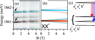
Figure 11: (color online) (a) Experimental and (b) simulated PL spectrum of XX^- in magnetic field in Faraday configuration. Color saturation denotes degree of linear polarization (red — $\vec{E}\parallel\vec{B}_{\mathrm{ext}}$, blue — $\vec{E}\perp\vec{B}_{\mathrm{ext}}$) and brightness denotes the PL intensity. A mismatch between orientation of magnetic field and the QD anisotropy was $16^{\circ}$. (c) Schematic of the corresponding energy diagram with the main recombination channels.

Finally, we studied the XX^- transition in the Voigt geometry. Both the experiment (Fig. 11(a)) and the model (Fig. 11(b)) show only small variation of the PL spectrum of XX^-. Interesting point in this configuration would be an observation of the transition leading to optically forbidden branch of the final state, in analogy to the dark neutral exciton, which is partially allowed by in-plane magnetic field. The transition would produce emission lines at energy approximately $\widetilde{\delta}_{0}$ above the higher energy component of the XX^- in the PL spectrum. No such lines were found experimentally. The reason is that in contrast to the case of neutral exciton, different lines of XX^- transition share the same initial state and a small admixture of optically allowed states is not sufficient to successfully compete with other radiative channels.

VI Summary

Basing on the set of different photoluminescence experiments we have extracted a key parameters describing properties of excitonic complexes in CdTe/ZnTe dots. The values of the parameters were analyzed statistically over the large number of different dots. The averaged values of the main parameters are summarized in Table 2.

Parameter	Value
$E_{XX}-E_{X}$	$\left(13.2\pm 1.3\right)$ meV
$\delta_{0}$	$\left(0.91\pm 0.13\right)$ meV
$\delta_{1}$	$\left(0.18\pm 0.11\right)$ meV
$\delta_{0}^{\mathrm{ps}}$	$\left(0.29\pm 0.08\right)$ meV
$\delta_{1}^{\mathrm{ps}}$	$\left(-0.49\pm 0.13\right)$ meV

Table 2: A summary of parameters describing CdTe/ZnTe QD emission spectrum. Symbols were explained in the text. Uncertainties of the listed values are related to the spread between individual dots. They in each case exceeded the experimental errors.

Despite large inhomogeneous broadening of QD emission in our samples, we demonstrate an universality of a single-dot emission spectrum with characteristic sequence of emission lines: X, X⁺, X^-, X^2- (two lines), XX, and XX^- (two lines). The fine structures of these transitions were successfully reproduced using an extension of the model developed by Bayer et al Bayer et al. (2002). The model involves exchange interaction between $s$-shell electron and hole as well as between $s$-shell hole and $p$-shell electron. We determined average values of parameters of these two interactions separately by analysis of the fine structure of X and X^2- transition respectively.

Independently, from the analysis of XX^- transition we have obtained effective exchange parameters $\widetilde{\delta_{0}}=\left(0.75\pm 0.16\right)$ meV and $\widetilde{\delta_{1}}=\left(-0.28\pm 0.08\right)$ meV. We compare these values with respective combination of $\delta_{i}$ and $\delta_{i}^{ps}$ parameters and find acceptable agreement between them. Such a comparison is an important test of the consistency of the model based solely on spin Hamiltonians.

The second important result of our work is a verification of the model calculations of excitonic transitions in the external magnetic field either in Faraday or Voigt configuration. Our findings clearly demonstrate that the measured transition energies as well as polarization selection rules perfectly follow the theoretical predictions. This agreement firmly supports applicability of the spin Hamiltonian model to the fine structure of states featuring also $p$-shell electrons.

Appendix A Hamiltonian operators

Here we describe the Hamiltonians used for the calculation of energies of excitonic states and transitions discussed in the manuscript. For the sake of transparency of the calculations, we have included only terms related to the observed effects. Namely, we included iso- and anisotropic e-h exchange interaction (described by $\delta_{0}$ and $\delta_{1}$ for interaction with s-shell and $\delta_{0}^{\mathrm{ps}}$ and $\delta_{1}^{\mathrm{ps}}$ for interaction with p-shell electron) and electron and hole g-factors (normal — $g_{e}^{\mathbf{z}}$ and $g_{h}^{\mathbf{z}}$; and in-plane — $g_{e}^{\mathbf{x},\mathbf{y}}$ and $g_{h}^{\mathbf{x},\mathbf{y}}$). We have neglected exchange interaction between $\uparrow\Uparrow$ and $\downarrow\Downarrow$ configurations ($\delta_{2}$ term), heavy-light hole mixing, orbital effects related to the p-shell (zero-field degeneracy, orbital angular momentum), anisotropy of e-e exchange interaction, and configuration mixing of exciton complexes due to direct Coulomb interactionHawrylak (1999). Furthermore, in the states containing two electrons (initial state of X^2- and final state of XX^- transition) we have assumed dominant role of electron-electron interaction and limited the analysis to the subspace corresponding to electron triplet configuration. The orientation of the in-plane QD anisotropy is arbitrarily chosen along the $x$ axis.

Eigenstates and their energies were obtained by analytical diagonalization . The only exception was the final state of XX^- transition with in-plane magnetic field for which which the 6$\times$6 eigenproblem was solved numerically.

Optical transitions were calculated using transition operators $P_{+}$ and $P_{-}$ corresponding to $\sigma_{+}$ and $\sigma_{-}$ polarization. We were not interested in the absolute values of the oscillator strength and took $P_{+(-)}=a_{s,\uparrow(\downarrow)}b_{s,\Downarrow(\Uparrow)}$ where $a$, $b$ are annihilation operators for electron and hole respectively. Intensity (relative) of PL line related to transition $\left|i\right>\to\left|f\right>$ was calculated as $\left|\langle f\mid\alpha P_{+}+\beta P_{-}\mid i\rangle\right|^{2}$ where parameters $\alpha$ and $\beta$ are defined by the polarization used in detection (e.g. $\alpha=1$, $\beta=0$ for $\sigma_{+}$ or $\alpha=\beta=\frac{1}{\sqrt{2}}$ for horizontal linear polarization). In such approach we did not analyze excitation dynamics nor the population effect on the PL intensity.

Below we explicitly present all matrices related to X^2- and XX^- transitions. The base states are given using a notation $\left|{{\mathrm{A}}\atop{\mathrm{B}}}\mathrm{C}\right>$, where A is related to $p$-shell electrons, B is related to $s$-shell electrons, and C is related to $s$-shell holes.

A.1 Matrices related to X^2- transition

Basis of the initial state:

$$\left|{{\uparrow}\atop{\uparrow\downarrow}}\Uparrow\right>,\ \left|{{\downarrow}\atop{\uparrow\downarrow}}\Uparrow\right>,\ \left|{{\uparrow}\atop{\uparrow\downarrow}}\Downarrow\right>,\ \left|{{\downarrow}\atop{\uparrow\downarrow}}\Downarrow\right>.$$

Basis of the final state:

$$\left|{{\uparrow}\atop{\uparrow}}\right>,\ \frac{1}{\sqrt{2}}\left(\left|{{\downarrow}\atop{\uparrow}}\right>+\left|{{\uparrow}\atop{\downarrow}}\right>\right),\ \left|{{\downarrow}\atop{\downarrow}}\right>.$$

Hamiltonian of the initial state of X^2- transition:

$$H_{i}=\frac{1}{2}\left(\begin{array}[]{cccc}-\delta_{0}^{ps}+\left(g_{e}^{\mathbf{z}}+g_{h}^{\mathbf{z}}\right)\mu_{B}B_{z}&g_{e}^{\mathbf{x}}\mu_{B}B_{x}-\mathbf{\imath}g_{e}^{\mathbf{y}}\mu_{B}B_{y}&g_{h}^{\mathbf{x}}\mu_{B}B_{x}-\mathbf{\imath}g_{h}^{\mathbf{y}}\mu_{B}B_{y}&0\\ g_{e}^{\mathbf{x}}\mu_{B}B_{x}+\mathbf{\imath}g_{e}^{\mathbf{y}}\mu_{B}B_{y}&\delta_{0}^{ps}+\left(-g_{e}^{\mathbf{z}}+g_{h}^{\mathbf{z}}\right)\mu_{B}B_{z}&\delta_{1}^{ps}&g_{h}^{\mathbf{x}}\mu_{B}B_{x}-\mathbf{\imath}g_{h}^{\mathbf{y}}\mu_{B}B_{y}\\ g_{h}^{\mathbf{x}}\mu_{B}B_{x}+\mathbf{\imath}g_{h}^{\mathbf{y}}\mu_{B}B_{y}&\delta_{1}^{ps}&\delta_{0}^{ps}+\left(g_{e}^{\mathbf{z}}-g_{h}^{\mathbf{z}}\right)\mu_{B}B_{z}&g_{e}^{\mathbf{x}}\mu_{B}B_{x}-\mathbf{\imath}g_{e}^{\mathbf{y}}\mu_{B}B_{y}\\ 0&g_{h}^{\mathbf{x}}\mu_{B}B_{x}+\mathbf{\imath}g_{h}^{\mathbf{y}}\mu_{B}B_{y}&g_{e}^{\mathbf{x}}\mu_{B}B_{x}+\mathbf{\imath}g_{e}^{\mathbf{y}}\mu_{B}B_{y}&-\delta_{0}^{ps}+\left(-g_{e}^{\mathbf{z}}-g_{h}^{\mathbf{z}}\right)\mu_{B}B_{z}\\ \end{array}\right)$$

Hamiltonian of the final state of X^2- transition:

$$H_{f}=\left(\begin{array}[]{ccc}g_{e}^{\mathbf{z}}\mu_{B}B_{z}&\frac{1}{\sqrt{2}}g_{e}^{\mathbf{x}}\mu_{B}B_{x}-\frac{\mathbf{\imath}}{\sqrt{2}}g_{e}^{\mathbf{y}}\mu_{B}B_{y}&0\\ \frac{1}{\sqrt{2}}g_{e}^{\mathbf{x}}\mu_{B}B_{x}+\frac{\mathbf{\imath}}{\sqrt{2}}g_{e}^{\mathbf{y}}\mu_{B}B_{y}&0&\frac{1}{\sqrt{2}}g_{e}^{\mathbf{x}}\mu_{B}B_{x}-\frac{\mathbf{\imath}}{\sqrt{2}}g_{e}^{\mathbf{y}}\mu_{B}B_{y}\\ 0&\frac{1}{\sqrt{2}}g_{e}^{\mathbf{x}}\mu_{B}B_{x}+\frac{\mathbf{\imath}}{\sqrt{2}}g_{e}^{\mathbf{y}}\mu_{B}B_{y}&-g_{e}^{\mathbf{z}}\mu_{B}B_{z}\end{array}\right)$$

Transition operators:

$$P_{+}=\left(\begin{array}[]{cccc}-1&0&0&0\\ 0&-\frac{1}{\sqrt{2}}&0&0\\ 0&0&0&0\end{array}\right)$$

$$P_{-}=\left(\begin{array}[]{cccc}0&0&0&0\\ 0&0&\frac{1}{\sqrt{2}}&0\\ 0&0&0&1\end{array}\right)$$

A.2 Matrices related to XX^- transition

Basis of the initial state:

$$\left|{{\uparrow}\atop{\uparrow\downarrow}}\Uparrow\Downarrow\right>,\ \left|{{\downarrow}\atop{\uparrow\downarrow}}\Uparrow\Downarrow\right>.$$

Basis of the final state:

$$\begin{array}[]{l}\left|{{\uparrow}\atop{\uparrow}}\Uparrow\right>,\ \frac{1}{\sqrt{2}}\left(\left|{{\downarrow}\atop{\uparrow}}\Uparrow\right>+\left|{{\uparrow}\atop{\downarrow}}\Uparrow\right>\right),\ \left|{{\downarrow}\atop{\downarrow}}\Uparrow\right>,\\ \left|{{\uparrow}\atop{\uparrow}}\Downarrow\right>,\ \frac{1}{\sqrt{2}}\left(\left|{{\downarrow}\atop{\uparrow}}\Downarrow\right>+\left|{{\uparrow}\atop{\downarrow}}\Downarrow\right>\right),\ \left|{{\downarrow}\atop{\downarrow}}\Downarrow\right>.\end{array}$$

Hamiltonian of the initial state of XX^- transition:

$$H_{i}=\frac{1}{2}\left(\begin{array}[]{cc}g_{e}^{\mathbf{z}}\mu_{B}B_{z}&g_{e}^{\mathbf{x}}\mu_{B}B_{x}-\mathbf{\imath}g_{e}^{\mathbf{y}}\mu_{B}B_{y}\\ g_{e}^{\mathbf{x}}\mu_{B}B_{x}+\mathbf{\imath}g_{e}^{\mathbf{y}}\mu_{B}B_{y}&-g_{e}^{\mathbf{z}}\mu_{B}B_{z}\end{array}\right)$$ (7)

Hamiltonian of the final state of XX^- transition:

$$H_{f}=\left(\begin{array}[]{cccccc}-\widetilde{\delta_{0}}+\xi_{e}^{\mathbf{z}}+\frac{1}{2}\xi_{h}^{\mathbf{z}}&\frac{1}{\sqrt{2}}\xi_{e}^{\mathbf{x}}-\frac{\mathbf{\imath}}{\sqrt{2}}\xi_{e}^{\mathbf{y}}&0&\frac{1}{2}\xi_{h}^{\mathbf{x}}-\frac{\mathbf{\imath}}{2}\xi_{h}^{\mathbf{y}}&0&0\\ \frac{1}{\sqrt{2}}\xi_{e}^{\mathbf{x}}+\frac{\mathbf{\imath}}{\sqrt{2}}\xi_{e}^{\mathbf{y}}&\frac{1}{2}\xi_{h}^{\mathbf{z}}&\frac{1}{\sqrt{2}}\xi_{e}^{\mathbf{x}}-\frac{\mathbf{\imath}}{\sqrt{2}}\xi_{e}^{\mathbf{y}}&\frac{1}{\sqrt{2}}\widetilde{\delta_{1}}&\frac{1}{2}\xi_{h}^{\mathbf{x}}-\frac{\mathbf{\imath}}{2}\xi_{h}^{\mathbf{y}}&0\\ 0&\frac{1}{\sqrt{2}}\xi_{e}^{\mathbf{x}}+\frac{\mathbf{\imath}}{\sqrt{2}}\xi_{e}^{\mathbf{y}}&\widetilde{\delta_{0}}-\xi_{e}^{\mathbf{z}}+\frac{1}{2}\xi_{h}^{\mathbf{z}}&0&\frac{1}{\sqrt{2}}\widetilde{\delta_{1}}&\frac{1}{2}\xi_{h}^{\mathbf{x}}-\frac{\mathbf{\imath}}{2}\xi_{e}^{\mathbf{y}}\\ \frac{1}{2}\xi_{h}^{\mathbf{x}}+\frac{\mathbf{\imath}}{2}\xi_{h}^{\mathbf{y}}&\frac{1}{\sqrt{2}}\widetilde{\delta_{1}}&0&\widetilde{\delta_{0}}+\xi_{e}^{\mathbf{z}}-\frac{1}{2}\xi_{h}^{\mathbf{z}}&\frac{1}{\sqrt{2}}\xi_{e}^{\mathbf{x}}-\frac{\mathbf{\imath}}{\sqrt{2}}\xi_{e}^{\mathbf{y}}&0\\ 0&\frac{1}{2}\xi_{h}^{\mathbf{x}}+\frac{\mathbf{\imath}}{2}\xi_{h}^{\mathbf{y}}&\frac{1}{\sqrt{2}}\widetilde{\delta_{1}}&\frac{1}{\sqrt{2}}\xi_{e}^{\mathbf{x}}+\frac{\mathbf{\imath}}{\sqrt{2}}\xi_{e}^{\mathbf{y}}&-\frac{1}{2}\xi_{h}^{\mathbf{z}}&\frac{1}{\sqrt{2}}\xi_{e}^{\mathbf{x}}-\frac{\mathbf{\imath}}{\sqrt{2}}\xi_{e}^{\mathbf{y}}\\ 0&0&\frac{1}{2}\xi_{h}^{\mathbf{x}}+\frac{\mathbf{\imath}}{2}\xi_{e}^{\mathbf{y}}&0&\frac{1}{\sqrt{2}}\xi_{e}^{\mathbf{x}}+\frac{\mathbf{\imath}}{\sqrt{2}}\xi_{e}^{\mathbf{y}}&-\widetilde{\delta_{0}}-\xi_{e}^{\mathbf{z}}-\frac{1}{2}\xi_{h}^{\mathbf{z}}\end{array}\right)$$ (8)

where $\xi_{i}^{\mathbf{j}}$ denotes $g_{i}^{\mathbf{j}}\mu_{B}B_{j}$ and $\widetilde{\delta_{i}}$ denotes $\frac{1}{2}\left(\delta_{i}+\delta_{i}^{ps}\right)$.

Transition operators:

$$P_{-}=\left(\begin{array}[]{cccc}0&0\\ 0&0\\ 0&0\\ -1&0\\ 0&-\frac{1}{\sqrt{2}}\\ 0&0\\ \end{array}\right),P_{+}=\left(\begin{array}[]{cc}0&0\\ -\frac{1}{\sqrt{2}}&0\\ 0&-1\\ 0&0\\ 0&0\\ 0&0\\ \end{array}\right).$$

Appendix B Polarization of XX^- lines in Faraday configuration

Below we give the analytical expressions describing the degree of circular polarization for each spectral line of XX^- transition in magnetic field in Faraday configuration. The Hamiltonians used to obtain these expressions were presented in Appendix A (Eq. 7 and 8). $P_{\mathrm{E}}$, $P_{\mathrm{F}}$, $P_{\mathrm{G}}$, and $P_{\mathrm{H}}$ denote circular polarization $P=\frac{I_{\sigma+}-I_{\sigma-}}{I_{\sigma+}+I_{\sigma-}}$ for the lines E, F, G, and H of XX^- transition as defined in Fig. 10.

$$P_{\mathrm{E}} = \frac{\left(\sqrt{2\beta^{2}+\left(\eta-1\right)^{2}}+\left(\eta-1\right)\right)^{2}-\beta^{2}}{\left(\sqrt{2\beta^{2}+\left(\eta-1\right)^{2}}+\left(\eta-1\right)\right)^{2}+\beta^{2}}$$ (9)

$$P_{\mathrm{F}} = \frac{\left(\sqrt{2\beta^{2}+\left(\eta+1\right)^{2}}+\left(\eta+1\right)\right)^{2}-4\beta^{2}}{\left(\sqrt{2\beta^{2}+\left(\eta+1\right)^{2}}+\left(\eta+1\right)\right)^{2}+4\beta^{2}}$$ (10)

$$P_{\mathrm{G}} = \frac{\left(\sqrt{2\beta^{2}+\left(\eta+1\right)^{2}}-\left(\eta+1\right)\right)^{2}-4\beta^{2}}{\left(\sqrt{2\beta^{2}+\left(\eta+1\right)^{2}}-\left(\eta+1\right)\right)^{2}+4\beta^{2}}$$ (11)

$$P_{\mathrm{H}} = \frac{\left(\sqrt{2\beta^{2}+\left(\eta-1\right)^{2}}-\left(\eta-1\right)\right)^{2}-\beta^{2}}{\left(\sqrt{2\beta^{2}+\left(\eta-1\right)^{2}}-\left(\eta-1\right)\right)^{2}+\beta^{2}}$$ (13)

where

$$\beta = \widetilde{\delta_{1}}/\widetilde{\delta_{0}}$$ (15)

$$\eta = \left(g_{e}^{\mathbf{z}}-g_{h}^{\mathbf{z}}\right)\mu_{B}B/\widetilde{\delta_{0}}$$ (16)

References

- Gammon et al. (1996) D. Gammon, E. S. Snow, B. V. Shanabrook, D. S. Katzer, and D. Park, Phys. Rev. Lett. 76, 3005 (1996).
- Benson et al. (2000) O. Benson, C. Santori, M. Pelton, and Y. Yamamoto, Phys. Rev. Lett. 84, 2513 (2000).
- Stevenson et al. (2006) R. M. Stevenson, R. J. Young, P. Atkinson, K. Cooper, D. A. Ritchie, and A. J. Shields, Nature 439, 179 (2006).
- Akopian et al. (2006) N. Akopian, N. H. Lindner, E. Poem, Y. Berlatzky, J. Avron, D. Gershoni, B. D. Gerardot, and P. M. Petroff, Phys. Rev. Lett. 96, 130501 (2006).
- Besombes et al. (2004) L. Besombes, Y. Léger, L. Maingault, D. Ferrand, H. Mariette, and J. Cibert, Phys. Rev. Lett. 93, 207403 (2004).
- Goryca et al. (2009) M. Goryca, T. Kazimierczuk, M. Nawrocki, A. Golnik, J. A. Gaj, P. Kossacki, P. Wojnar, and G. Karczewski, Phys. Rev. Lett. 103, 087401 (2009).
- Goryca et al. (2010) M. Goryca, P. Plochocka, T. Kazimierczuk, P. Wojnar, G. Karczewski, J. A. Gaj, M. Potemski, and P. Kossacki, Phys. Rev. B 82, 165323 (2010).
- Urbaszek et al. (2003) B. Urbaszek, R. J. Warburton, K. Karrai, B. D. Gerardot, P. M. Petroff, and J. M. Garcia, Phys. Rev. Lett. 90, 247403 (2003).
- Akimov et al. (2005) I. A. Akimov, K. V. Kavokin, A. Hundt, and F. Henneberger, Phys. Rev. B 71, 075326 (2005).
- Cade et al. (2006) N. I. Cade, H. Gotoh, H. Kamada, H. Nakano, and H. Okamoto, Phys. Rev. B 73, 115322 (2006).
- Ediger et al. (2007) M. Ediger, G. Bester, B. D. Gerardot, A. Badolato, P. M. Petroff, K. Karrai, A. Zunger, and R. J. Warburton, Phys. Rev. Lett. 98, 036808 (2007).
- Hawrylak (1999) P. Hawrylak, Phys. Rev. B 60, 5597 (1999).
- Tinjod et al. (2003) F. Tinjod, B. Gilles, S. Moehl, K. Kheng, and H. Mariette, Applied Physics Letters 82, 4340 (2003).
- Wojnar et al. (2008) P. Wojnar, J. Suffczyński, K. Kowalik, A. Golnik, M. Aleszkiewicz, G. Karczewski, and J. Kossut, Nanotechnology 19, 235403 (2008).
- Suffczyński et al. (2006) J. Suffczyński, T. Kazimierczuk, M. Goryca, B. Piechal, A. Trajnerowicz, K. Kowalik, P. Kossacki, A. Golnik, K. P. Korona, M. Nawrocki, et al., Phys. Rev. B 74, 085319 (2006).
- Léger et al. (2007) Y. Léger, L. Besombes, L. Maingault, and H. Mariette, Phys. Rev. B 76, 045331 (2007).
- Lee et al. (2009) H. S. Lee, A. Rastelli, M. Benyoucef, F. Ding, T. W. Kim, H. L. Park, and O. G. Schmidt, Nanotechnology 20, 075705 (2009).
- Léger et al. (2006) Y. Léger, L. Besombes, J. Fernández-Rossier, L. Maingault, and H. Mariette, Phys. Rev. Lett. 97, 107401 (2006).
- Kazimierczuk et al. (2009a) T. Kazimierczuk, J. Suffczynski, A. Golnik, J. A. Gaj, P. Kossacki, and P. Wojnar, Phys. Rev. B 79, 153301 (2009a).
- Cortez et al. (2002) S. Cortez, O. Krebs, S. Laurent, M. Senes, X. Marie, P. Voisin, R. Ferreira, G. Bastard, J.-M. Gérard, and T. Amand, Phys. Rev. Lett. 89, 207401 (2002).
- Dzhioev et al. (2002) R. I. Dzhioev, V. L. Korenev, B. P. Zakharchenya, D. Gammon, A. S. Bracker, J. G. Tischler, and D. S. Katzer, Phys. Rev. B 66, 153409 (2002).
- Akimov et al. (2006) I. A. Akimov, D. H. Feng, and F. Henneberger, Phys. Rev. Lett. 97, 056602 (2006).
- Kazimierczuk et al. (2010) T. Kazimierczuk, M. Goryca, M. Koperski, A. Golnik, J. A. Gaj, M. Nawrocki, P. Wojnar, and P. Kossacki, Phys. Rev. B 81, 155313 (2010).
- Haas et al. (2009) K. Haas, T. Kazimierczuk, P. Wojnar, A. Golnik, J. Gaj, and P. Kossacki, Acta Phys. Pol. A 116, 896 (2009).
- Kudelski et al. (2001) A. Kudelski, A. Golnik, J. A. Gaj, F. V. Kyrychenko, G. Karczewski, T. Wojtowicz, Y. G. Semenov, O. Krebs, and P. Voisin, Phys. Rev. B 64, 045312 (2001).
- Bayer et al. (2002) M. Bayer, G. Ortner, O. Stern, A. Kuther, A. A. Gorbunov, A. Forchel, P. Hawrylak, S. Fafard, K. Hinzer, T. L. Reinecke, et al., Phys. Rev. B 65, 195315 (2002).
- Poem et al. (2010) E. Poem, Y. Kodriano, C. Tradonsky, N. H. Lindner, B. D. Gerardot, P. M. Petroff, and D. Gershoni, Nature Physics 6, 993 (2010).
- Kudelski et al. (2000) A. Kudelski et al., in Proceedings of the 25th International Conference on Physics of Semiconductors (Springer, 2000), p. 1249.
- Kowalik et al. (2007) K. Kowalik, O. Krebs, A. Golnik, J. Suffczyński, P. Wojnar, J. Kossut, J. A. Gaj, and P. Voisin, Phys. Rev. B 75, 195340 (2007).
- Kazimierczuk et al. (2009b) T. Kazimierczuk, A. Golnik, M. Goryca, P. Wojnar, J. Gaj, and P. Kossacki, Acta Phys. Pol. A 116, 882 (2009b).
- Poem et al. (2007) E. Poem, J. Shemesh, I. Marderfeld, D. Galushko, N. Akopian, D. Gershoni, B. D. Gerardot, A. Badolato, and P. M. Petroff, Phys. Rev. B 76, 235304 (2007).
- Finley et al. (2001) J. J. Finley, P. W. Fry, A. D. Ashmore, A. Lemaître, A. I. Tartakovskii, R. Oulton, D. J. Mowbray, M. S. Skolnick, M. Hopkinson, P. D. Buckle, et al., Phys. Rev. B 63, 161305 (2001).