Effective speed of sound in phononic crystals

Abstract

A new formula for the effective quasistatic speed of sound $c$ in 2D and 3D periodic materials is reported. The approach uses a monodromy-matrix operator to enable direct integration in one of the coordinates and exponentially fast convergence in others. As a result, the solution for $c$ has a more closed form than previous formulas. It significantly improves the efficiency and accuracy of evaluating $c$ for high-contrast composites as demonstrated by a 2D example with extreme behavior.

I Introduction

Long-standing interest in modelling effective elastic properties of composites with microstructure has substantially intensified with the emerging possibility of designing periodic structures in air DT and in solids MLWS to form phononic crystals and other exotic metamaterials, which open up exciting application prospects ranging from negative index lenses to small scale multiband phononic devicesV-H . This new prospective brings about the need for fast and accurate computational schemes to test ideas in silico. The most common numerical tool is the Fourier or plane-wave expansion method (PWE). It is widely used for calculating various spectral parameters including the effective quasistatic speed of sound in acoustic KAG and elastic QN phononic crystals. At the same time, the PWE calculation is known to face problems when applied to high-contrast composites V-H , which are of especial interest for applications. Particularly riveting is the case where a soft ingredient is embedded in a way breaking the connectivity of densely packed regions of stiff ingredient. Physically speaking, the speed of sound, which is large in a homogeneously stiff medium, should fall dramatically when even a small amount of soft component forms a ’quasi-insulating network’. Note that this case, which implies a strong effect of multiple interactions, is also ungainly for the multiple-scattering approach DT ; MLWS .

The purpose of present Letter is to highlight a new method for evaluating the quasistatic effective sound speed $c$ in 2D and 3D phononic crystals. The idea is to recast the wave equation as a 1st-order ’ordinary’ differential system (ODS) with respect to one coordinate (say $x_{1}$) and to use a monodromy-matrix operator defined as a multiplicative (or path) integral in $x_{1}$. By this means, we derive a formula for $c$ whose essential advantages are an explicit integration in $x_{1}$ and an exponentially small error of truncation in other coordinate(s). Both these features of the analytical result are shown to significantly improve the efficiency and accuracy of its numerical implementation in comparison with the conventional PWE calculation, which is demonstrated for a 2D steel/epoxy square lattice. The power of the new approach is especially apparent at high concentration $f$ of steel inclusions, where the effective speed $c$ displays a steep, near vertical, dependence for $f\approx 1$, a feature not captured by conventional techniques like PWE.

II Effective speed: 2D acoustic waves

A. SETUP. Consider the scalar wave equation

$$\boldsymbol{\nabla}\cdot\left(\mu\boldsymbol{\nabla}v\right)=-\rho\omega^{2}v,$$ (1)

for time-harmonic shear displacement $v(\mathbf{x},t)=v(\mathbf{x})e^{-i\omega t}$ in a 2D solid continuum with $\mathbf{T}$-periodic density $\rho(\mathbf{x})$ and shear coefficient $\mu(\mathbf{x})$. Assume a square unit cell $\mathbf{T}=\sum_{i}t_{i}\mathbf{a}_{i}=\left[0,1\right]^{2}$ with unit translation vectors $\mathbf{a}_{1}\perp\mathbf{a}_{2}$ taken as the basis for $\mathbf{x}=\sum_{i}x_{i}\mathbf{a}_{i}.$ Imposing the Floquet condition $v(\mathbf{x})=u(\mathbf{x})e^{i\mathbf{k\cdot x}}$ where $u(\mathbf{x})$ is periodic and $\mathbf{k}=k\boldsymbol{\kappa}$ ($\left|\boldsymbol{\kappa}\right|=1$), Eq. (1) becomes

$$({\mathcal{C}}_{0}+{\mathcal{C}}_{1}+{\mathcal{C}}_{2})u=\rho\omega^{2}u\ \ \mathrm{with\ }{\mathcal{C}}_{0}u=-\boldsymbol{\nabla}(\mu\boldsymbol{\nabla}u),$$

$${\mathcal{C}}_{1}u=-i\mathbf{k}\cdot(\mu\boldsymbol{\nabla}u+\boldsymbol{\nabla}(\mu u)),\ \ {\mathcal{C}}_{2}u=k^{2}\mu u.$$ (2)

Regular perturbation theory applied to (2) yields the effective speed $c(\boldsymbol{\kappa})=\lim_{\omega,k\rightarrow 0}\omega(\mathbf{k})/k$ in the form KSAP

$$c^{2}(\boldsymbol{\kappa})=\mu_{\mathrm{eff}}(\boldsymbol{\kappa})/\langle\rho\rangle,\ \mu_{\mathrm{eff}}(\boldsymbol{\kappa})=\left\langle\mu\right\rangle-M(\boldsymbol{\kappa})\ \mathrm{with}$$ (3)

$$M(\boldsymbol{\kappa})=\begin{matrix}\sum\nolimits_{i,j=1}^{2}\end{matrix}M_{ij}\kappa_{i}\kappa_{j},\ M_{ij}=\left({\mathcal{C}}_{0}^{-1}\partial_{i}\mu,\partial_{j}\mu\right)=M_{ji},$$

where $\partial_{i}\equiv\partial/\partial x_{i}$, spatial averages are defined by

$$\left\langle f\right\rangle\equiv\begin{matrix}\int_{\mathbf{T}}\end{matrix}f(\mathbf{x})\mathrm{d}\mathbf{x\ }\ \big{(}=\left\langle\left\langle f\right\rangle_{1}\right\rangle_{2},\mathbf{\ }\left\langle f\right\rangle_{i}\equiv\begin{matrix}\int_{0}^{1}\end{matrix}f(\mathbf{x})\mathrm{d}x_{i}\big{)},$$ (4)

and $(\cdot,\cdot)$ denotes the scalar product in $L^{2}(\mathbf{T})$ so that $(f,h)=\left\langle fh^{\ast}\right\rangle$ (^∗ means complex conjugation). The difficulty with (3) is that it involves the inverse of a partial differential operator ${\mathcal{C}}_{0}$. One solution is to apply a double Fourier expansion to ${\mathcal{C}}_{0}^{-1}$ and $\partial_{i}\mu$ in (3). This leads to the PWE formula for the effective speedKAG which is expressed via infinite vectors and the inverse of the infinite matrix of Fourier coefficients of $\mu(\mathbf{x})$. Numerical implementation of the PWE formula requires dealing with large dense matrices, especially in the case of high-contrast composites for which the PWE convergence is slow (see §IV). An alternative ”brute force” procedure of the scaling approach is to numerically solve the partial differential equation ${\mathcal{C}}_{0}h=\partial_{i}\mu$ for the $\mathbf{1}$-periodic function $h(\mathbf{x})$ (e.g. via the boundary integral methodAADW ).

The new approach proposed here leads to a more efficient formula for $c$ based on direct analytical integration in one coordinate direction. There are two ways of doing so. The first proceeds from the ODS form of the wave equation (1) itself, which means ’skipping’ (3). This is convenient for deriving $c(\boldsymbol{\kappa})$ in the principal directions $\boldsymbol{\kappa}\parallel\mathbf{a}_{1,2},$ see §IIB. The second method is more closely related to the conventional PWE and scaling approaches in that it also starts from (3) but treats it differently, namely, the equation ${\mathcal{C}}_{0}h=\partial_{i}\mu$ is cast in ODS form and analytically integrated in one coordinate. This is basically equivalent to the former method, but enables an easier derivation of the off-diagonal component $M_{12}$ for the anisotropic case, see §IIC.

B. Wave speed in the principal directions. The wave equation (1) may be recast as

$$\boldsymbol{\eta}^{\prime}=\mathcal{Q}\boldsymbol{\eta}\quad\mathrm{with}\ \ \mathcal{A=}-\partial_{2}(\mu\partial_{2}),~{}$$

$$\mathcal{Q}=\begin{pmatrix}0&\mu^{-1}\\ \mathcal{A}-\rho\omega^{2}&0\end{pmatrix},\ \boldsymbol{\eta}(\mathbf{x})=\begin{pmatrix}v\\ \mu v^{\prime}\end{pmatrix},\$$ (5)

where $\prime$ stands for $\partial_{1}$. The solution to Eq. (5) for initial data $\boldsymbol{\eta}(0,x_{2})\equiv\boldsymbol{\eta}(0,\cdot)$ at $x_{1}=0$ is

$$\boldsymbol{\eta}(x_{1},\cdot)=\mathcal{M}\left[x_{1},0\right]\boldsymbol{\eta}(0,\cdot)\ \mathrm{with}$$

$$\mathcal{M}\left[a,b\right]=\begin{matrix}\widehat{\int}_{b}^{a}\end{matrix}(\mathcal{I}+\mathcal{Q}\mathrm{d}x_{1}).$$ (6)

The operator $\mathcal{M}\left[x_{1},0\right]$ is formally the matricant, or propagator, of (5) defined through the multiplicative integral $\widehat{\int}$ (with $\mathcal{I}$ denoting the identity operator). It is assumed for the moment that $\rho(\mathbf{x})$ and $\mu(\mathbf{x})$ are smooth to ensure the existence of $\mathcal{M}$. The matricant over a period, $\mathcal{M}\left[1,0\right]$, is called the monodromy matrix.

Assume the Floquet condition with the wave vector $\mathbf{k}=(k_{1}\ 0)^{\mathrm{T}}$ so that $v(\mathbf{x})=u(\mathbf{x})e^{ik_{1}x_{1}}$ and $\boldsymbol{\eta}(1,\cdot)$ $=\boldsymbol{\eta}(0,\cdot)e^{ik_{1}}.$ By (6)₁, this implies the eigenproblem

$$\mathcal{M}\left[1,0\right]\mathbf{w}(k_{1})=e^{ik_{1}}\mathbf{w}(k_{1}).$$ (7)

where $\mathcal{M}\left[1,0\right]$ depends on $\omega$. Eq. (7) defines $k_{1}=k_{1}(\omega)$ and hence $\omega=\omega(k_{1}),$ where $\omega^{2}$ is the eigenvalue of (1) with $v(\mathbf{x})=u(\mathbf{x})e^{ik_{1}x_{1}}$. The effective speed $c(\kappa_{1})=\lim_{\omega,k_{1}\rightarrow 0}\omega/k_{1}$ can therefore be determined by applying perturbation theory to (7) as $\omega,k_{1}\rightarrow 0$. The asymptotic form of $\mathcal{M}\left[1,0\right]$ follows from definitions (5) and (6)₂ as

$$\mathcal{M}\left[1,0\right]=\mathcal{M}_{0}+\omega^{2}\mathcal{M}_{1}+O(\omega^{4})\ \mathrm{where:}$$

$$\mathcal{M}_{0}\equiv\mathcal{M}_{0}\left[1,0\right],\ \mathcal{M}_{0}\left[a,b\right]=\begin{matrix}\widehat{\int}_{b}^{a}\end{matrix}(\mathcal{I}+\mathcal{Q}_{0}\mathrm{d}x_{1})\ \mathrm{with}\$$

$$\mathcal{Q}_{0}\equiv\mathcal{Q}_{\omega=0}=\begin{pmatrix}0&\mu^{-1}\\ \mathcal{A}&0\end{pmatrix},$$ (8)

$$\mathcal{M}_{1}=\int_{0}^{1}\mathcal{M}_{0}\left[1,x_{1}\right]\begin{pmatrix}0&0\\ -\rho&0\end{pmatrix}\mathcal{M}_{0}\left[x_{1},0\right]\mathrm{d}x_{1}.$$

Note the identities $\mathcal{Q}_{0}\mathbf{w}_{0}=\mathbf{0},\ \mathcal{Q}_{0}^{+}\widetilde{\mathbf{w}}_{0}=\mathbf{0}$ and hence

$$\mathcal{M}_{0}\left[a,b\right]\mathbf{w}_{0}=\mathbf{w}_{0},\ \mathcal{M}_{0}^{+}\left[a,b\right]\widetilde{\mathbf{w}}_{0}=\widetilde{\mathbf{w}}_{0}\mathbf{\ }\ (\forall a,b)$$

$$\mathrm{for}\ \mathbf{w}_{0}=(1\ 0)^{\mathrm{T}},\ \widetilde{\mathbf{w}}_{0}=(0\ 1)^{\mathrm{T}}.$$ (9)

By (9)₁ $\mathbf{w}_{0}$ is an eigenvector of $\mathcal{M}_{0}$ with the eigenvalue 1, and it can be shown to be a single eigenvector. Therefore $\mathbf{w}(k_{1})=\mathbf{w}_{0}+k_{1}\mathbf{w}_{1}+k_{1}^{2}\mathbf{w}_{2}+O(k_{1}^{3})$ and$\ \omega=ck_{1}+O(k_{1}^{2})$. Insert these expansions along with (8)₁ in (7) and collect the first-order terms in $k_{1}$ to obtain

$$\mathcal{M}_{0}\mathbf{w}_{1}=\mathbf{w}_{1}+i\mathbf{w}_{0}\ \Rightarrow\ \mathbf{w}_{1}=i(\mathcal{M}_{0}-\mathcal{I})^{-1}\mathbf{w}_{0}.$$ (10)

According to (9), $\mathcal{M}_{0}-\mathcal{I}$ has no inverse but is a one-to-one mapping from the subspace orthogonal to $\mathbf{w}_{0}$ onto the subspace orthogonal $\widetilde{\mathbf{w}}_{0};$ hence, $\mathbf{w}_{1}$ exists and $\widetilde{\mathbf{w}}_{0}\cdot\mathbf{w}_{1}$ is uniquely defined. The terms of second-order in $k_{1}$ in (7) then imply

$$\mathcal{M}_{0}\mathbf{w}_{2}+c^{2}\mathcal{M}_{1}\mathbf{w}_{0}=i\mathbf{w}_{1}+\mathbf{w}_{2}.$$ (11)

Scalar multiplication on both sides by $\widetilde{\mathbf{w}}_{0}$ leads, with account for (9) and (8)₄, to $c^{2}\langle\rho\rangle=-i\left\langle\widetilde{\mathbf{w}}_{0}\cdot\mathbf{w}_{1}\right\rangle_{2}$, whence by (10₂)

$$c^{2}(\kappa_{1})=\ \langle\rho\rangle^{-1}\left\langle\widetilde{\mathbf{w}}_{0}\cdot(\mathcal{M}_{0}-\mathcal{I})^{-1}\mathbf{w}_{0}\right\rangle_{2},$$ (12)

where the notation $\left\langle\cdot\right\rangle_{2}$ is explained in (4). Interchanging variables $x_{1}\rightleftarrows x_{2}$ in the above derivation yields a similar result for $c(\kappa_{2})$ as follows

$$c^{2}(\kappa_{2})=\left\langle\rho\right\rangle^{-1}\left\langle\widetilde{\mathbf{w}}_{0}\cdot(\widetilde{\mathcal{M}}_{0}-\mathcal{I})^{-1}\mathbf{w}_{0}\right\rangle_{1}\ \ \mathrm{where}$$

$$\widetilde{\mathcal{M}}_{0}=\begin{matrix}\widehat{\int}_{0}^{1}\end{matrix}(\mathcal{I}+\widetilde{\mathcal{Q}}_{0}\mathrm{d}x_{2}),$$ (13)

$$\widetilde{\mathcal{Q}}_{0}=\begin{pmatrix}0&\mu^{-1}\\ \widetilde{\mathcal{A}}&0\end{pmatrix},\ \ \widetilde{\mathcal{A}}=-\partial_{1}\mu\partial_{1}.$$

The result for a rectangular lattice with $\mathbf{T}=\left[0,T_{1}\right]\times\left[0,T_{2}\right]$ is obtained by replacing $x_{i}$ with $x_{i}/T_{i}.$

C. The full matrix $M_{ij}$. The anisotropy of the effective speed $c(\boldsymbol{\kappa}),$ i.e. its dependence on the wave normal $\boldsymbol{\kappa}\equiv\mathbf{k/}k$, is determined by the quadratic form $M(\boldsymbol{\kappa})=\sum\nolimits_{i,j=1}^{2}M_{ij}\kappa_{i}\kappa_{j}$ (see Eq. (3)), and represented by the ellipse of (squared) slowness $c^{-2}(\mathbf{\kappa})$. Eqs. (12) and (13)₁, which define $c(\kappa_{i})$ and so $M_{ii}$, suffice for the case where $\mathbf{T}$ is rectangular and $\mu(\mathbf{x})$ is even in (at least) one of $x_{i}$ so that the effective-slowness ellipse is $c^{-2}(\boldsymbol{\kappa})=\sum\nolimits_{i=1,2}c^{-2}(\kappa_{i})\kappa_{i}^{2}$ with the principal axes parallel to $\mathbf{a}_{1}\perp\mathbf{a}_{2}$. Otherwise $c(\boldsymbol{\kappa})$ for arbitrary $\boldsymbol{\kappa}$ requires finding the off-diagonal component $M_{12}$. For this purpose, with reference to (3), consider the equation

$${\mathcal{C}}_{0}h=\partial_{1}\mu$$ (14)

for $\mathbf{1}$-periodic $h(\mathbf{x})$. With the above notations this can be written as $-(\mu h^{\prime})^{\prime}+\mathcal{A}h=\mu^{\prime}$ or, more conveniently, $(\mu\widetilde{h}^{\prime})^{\prime}=\mathcal{A}\widetilde{h}$ with  $\widetilde{h}=h+x_{1}$. The latter is equivalent to

$$\boldsymbol{\xi}^{\prime}=\mathcal{Q}_{0}\boldsymbol{\xi}\mathrm{\ \ where\ }\boldsymbol{\ \xi}=\begin{pmatrix}h+x_{1}\\ \mu(h^{\prime}+1)\end{pmatrix}$$ (15)

and $\mathcal{Q}_{0}$ is given in (8)₃. The general solution to (15) is

$$\boldsymbol{\xi}(x_{1},\cdot)=\mathcal{M}_{0}\left[x_{1},0\right]\boldsymbol{\xi}(0,\cdot),$$ (16)

where $\mathcal{M}_{0}\left[x_{1},0\right]$ is defined in (8)₂, and $\boldsymbol{\xi}(0,\cdot)$ is the initial data at $x_{1}=0$. The periodicity of $h$ implies $\boldsymbol{\xi}(1,\cdot)=\boldsymbol{\xi}(0,\cdot)+\mathbf{w}_{0},$ while $\boldsymbol{\xi}(1,\cdot)=\mathcal{M}_{0}\boldsymbol{\xi}(0,\cdot)$ by (16). Hence $\boldsymbol{\xi}(0,\cdot)=(\mathcal{M}_{0}-\mathcal{I})^{-1}\mathbf{w}_{0}$ and so (14) is solved by

$$\boldsymbol{\xi}(x_{1},\cdot)=\mathcal{M}_{0}\left[x_{1},0\right](\mathcal{M}_{0}-\mathcal{I})^{-1}\mathbf{w}_{0}.$$ (17)

Substituting (17) into the definition of $M_{12}$ in (3) yields

$$M_{12} =(\mathcal{C}_{0}^{-1}\partial_{1}\mu,\partial_{2}\mu)=\langle h\partial_{2}\mu\rangle=\left\langle\partial_{2}\mu\mathbf{w}_{0}\cdot\boldsymbol{\xi}\right\rangle$$

$$=\left\langle\partial_{2}\mu\mathbf{w}_{0}\cdot\mathcal{M}_{0}[x_{1},0](\mathcal{M}_{0}-\mathcal{I})^{-1}\mathbf{w}_{0}\right\rangle.$$ (18)

Note that the formula (18) for $M_{12}$ requires more computation than the formulas (12) and (13)₁ for $M_{ii}$. Interestingly, if the unit cell $\mathbf{T}$ is square, then, for an arbitrary (periodic) $\mu(\mathbf{x})$, Eq. (18) can be circumvented by using the identity $M_{12}=(\widetilde{M}_{11}-\widetilde{M}_{22})/2$, where $\widetilde{M}_{ii}$ follow from Eqs. (12) and (13)₁ applied to the square lattice obtained from the given one by turning it 45^∘.

D. Discussion. The two lines of attack outlinedmentioned in §II.A are equivalent in that the formula (12) for the effective speed $c(\kappa_{1})$ in the principal direction can also be inferred from Eq. (3). Inserting the solution (17) of (14) defines the component $M_{11}$ as

$$M_{11}=\big{(}{\mathcal{C}}_{0}^{-1}\partial_{1}\mu,\partial_{1}\mu\big{)}=\langle h\mu^{\prime}\rangle=\langle\mu^{\prime}{\mathbf{w}}_{0}\cdot\boldsymbol{\xi}\rangle-\langle x_{1}\mu^{\prime}\rangle.$$ (19)

Integrating by parts each term in the last identity and using the periodicity of $\mu(\mathbf{x})$ along with Eqs. (8)₃, (9), (15)-(17) (see also the notation (4)) yields

$$\langle\mu^{\prime}{\mathbf{w}}_{0}\cdot\boldsymbol{\xi}\rangle=-\langle\widetilde{\mathbf{w}}_{0}\cdot(\mathcal{M}_{0}-\mathcal{I})^{-1}\mathbf{w}_{0}\rangle_{2}+\langle\mu(0,x_{2})\rangle_{2},$$

$$-\langle x_{1}\mu^{\prime}\rangle=\langle\mu\rangle-\langle\mu(1,x_{2})\rangle_{2}=\langle\mu\rangle-\langle\mu(0,x_{2})\rangle_{2}.$$ (20)

Thus, $M_{11}$$=\langle\mu\rangle$$-\left\langle\widetilde{\mathbf{w}}_{0}\cdot(\mathcal{M}_{0}-\mathcal{I})^{-1}\mathbf{w}_{0}\right\rangle_{2}$ which leads to (12), QED. Note that Eq. (18) is also obtainable via the monodromy matrix of the wave equation (1) (the approach of §IIB) with $v(\mathbf{x})=u(\mathbf{x})e^{i\mathbf{k\cdot x}}$ and $\mathbf{k\nparallel a}_{i},$ but this method of derivation of $M_{12}$ is lengthier than in §IIC.

As another remark, it is instructive to recover a known result for the case where $\mu(\mathbf{x})$ is periodic in one coordinate and does not depend on the other, say $\mu(x_{1},x_{2})=\mu(x_{1})$. Using (8)₂, (8)₃ and (13)₃ gives

$$(\mathcal{M}_{0}-\mathcal{I})\begin{pmatrix}0\\ \langle\mu^{-1}\rangle_{1}^{-1}\end{pmatrix}=\mathbf{w}_{0},~{}(\widetilde{\mathcal{M}}_{0}-\mathcal{I})\begin{pmatrix}0\\ \mu(x_{1})\end{pmatrix}=\mathbf{w}_{0}.$$ (21)

Therefore, by (12) and (13)₁, $c^{2}(\kappa_{1})=\langle\mu^{-1}\rangle_{1}^{-1}/\left\langle\rho\right\rangle$ and $c^{2}(\kappa_{2})=\langle\mu\rangle_{1}/\left\langle\rho\right\rangle$ while $M_{12}=0$ by (18) with $\partial_{2}\mu=0$.

Finally, we note that, while the above evaluation of quasistatic speed $c$ is exact, using the same monodromy-matrix approach also provides a closed-form approximation of $c.$ For the isotropic case, it is as follows (see KSAP for more details):

$$c^{2}\approx\frac{1}{2\left\langle\rho\right\rangle}\left(\left\langle\left\langle\mu^{-1}\right\rangle_{1}^{-1}\right\rangle_{2}+\left\langle\left\langle\mu\right\rangle_{2}^{-1}\right\rangle_{1}^{-1}\right).$$ (22)

III Effective speeds in principal directions for 3D elastic waves

The equation for time-harmonic elastic wave motion $\mathbf{v}(\mathbf{x},t)$$=$$\mathbf{v}(\mathbf{x})e^{-i\omega t}$ is, with repeated suffices summed,

$$-\partial_{j}(c_{ijkl}\partial_{l}v_{k})=\rho\omega^{2}v_{i}\ (i,j,k,l=1,2,3),$$ (23)

where density $\rho(\mathbf{x})$ and compliances $c_{ijkl}(\mathbf{x})$ are $\mathbf{T}$-periodic in a 3D periodic medium. Assume a cubic unit cell $\mathbf{T}=\sum_{i}t_{i}\mathbf{a}_{i}=\left[0,1\right]^{3}$ and refer the components $x_{i},~{}v_{i}$ and $c_{ijkl}$ to the orthogonal basis formed by the translation vectors $\mathbf{a}_{i}$. Impose the condition $\mathbf{v}(\mathbf{x})=\mathbf{u}(\mathbf{x})e^{i\mathbf{k\cdot x}}$ with periodic $\mathbf{u}(\mathbf{x})=(u_{i})$ and take $\mathbf{k}$ parallel to one of $\mathbf{a}_{i}$, e.g. to $\mathbf{a}_{1}$. Eq. (23) may be rewritten in the form

$$\boldsymbol{\eta}^{\prime}=\mathcal{Q}\boldsymbol{\eta}\ \ \mathrm{with}\ \ \boldsymbol{\eta}(\mathbf{x})=\begin{pmatrix}(u_{i})\\ (c_{i1kl}\partial_{l}u_{k})\end{pmatrix},$$

$$\mathcal{Q}=\begin{pmatrix}-\mathcal{C}^{-1}\mathcal{A}_{1}&\mathcal{C}^{-1}\\ \omega^{2}\rho\delta_{ij}+\mathcal{A}_{2}-\mathcal{A}_{1}\mathcal{C}^{-1}\mathcal{A}_{1}&\mathcal{A}_{1}\mathcal{C}^{-1}\end{pmatrix}$$ (24)

where the self-adjoint matrix operators $\mathcal{C}$ and $\mathcal{A}_{1,2}$ are

$$\mathcal{C}=(c_{i1k1}),\ \ \mathcal{A}_{1}(u_{i})=(c_{i1ka}\partial_{a}u_{k}),$$

$$\mathcal{A}_{2}(u_{i})=(\partial_{a}(c_{iakb}\partial_{b}u_{k}))\ \mathrm{with}\ \ \ a,b=2,3.$$ (25)

Like in the 2D case, denote the monodromy matrix for (24) at $\omega=0$ by $\mathcal{M}_{0}=\widehat{\int}_{0}^{1}(\mathcal{I}+\mathcal{Q}_{0}dx_{1})$ where $\mathcal{Q}_{0}=\mathcal{Q}_{\omega=0}$, and also introduce the 6$\times$3 matrices $\mathbf{W}_{0}=(\delta_{ij}~{}\mathbf{0})^{\mathrm{T}}$ and $\widetilde{\mathbf{W}}_{0}=(\mathbf{0\ }\delta_{ij})^{\mathrm{T}}$. Reasoning similar to that in §II.C leads us to the conclusion that the effective speeds $c_{\alpha}(\kappa_{1})=\lim_{\omega,k_{1}\rightarrow 0}\omega/k_{1}$ $(\alpha=1,2,3)$ of the three waves with $\mathbf{k}\equiv k\boldsymbol{\kappa}$ parallel to $\mathbf{a}_{1}$ are the eigenvalues of the 3$\times$3 matrix

$$\left\langle\left\langle\widetilde{\mathbf{W}}_{0}\cdot(\mathcal{M}_{0}-\mathcal{I})^{-1}\mathbf{W}_{0}\right\rangle_{2}\right\rangle_{3}\ \big{(}\mathrm{with}\ \langle\cdot\rangle_{i}\equiv(\ref{6.1})\big{)}.$$ (26)

IV Numerical implementation

There are several ways to use the above analytical results for calculating the effective speed. One approach is to transform to Fourier space with respect to coordinate(s) other than the coordinate of integration in the monodromy matrix. Consider the 2D case and apply the Fourier expansion $f(x_{1},x_{2})=\sum_{n\in\mathbb{Z}}\widehat{f}_{n}(x_{1})e^{2\pi inx_{2}}$ in $x_{2}$ for the functions $f=\mu$ and $\mu^{-1}$. Then the operator of multiplying by the function $\mu^{-1}(x_{1},\cdot)$ and the differential operator $\mathcal{A}(x_{1})\mathcal{=-\partial}_{2}(\mu(x_{1},\cdot)\mathcal{\partial}_{2})$ become matrices

$$\mu^{-1}\longmapsto\boldsymbol{\mu}^{-1}(x_{1})=(\widehat{\mu^{-1}}_{n-m})=(\widehat{\mu}_{n-m})^{-1},$$

$$\mathcal{A}\longmapsto\mathbf{A}(x_{1})=4\pi^{2}(nm\widehat{\mu}_{n-m}),\ n,m\in\mathbb{Z},$$ (27)

and Eq. (12) reduces to following form

$$c^{2}(\kappa_{1}) =\langle\rho\rangle^{-1}\widetilde{\mathbf{w}}_{\widehat{0}}\cdot(\mathbf{M}_{0}-\mathbf{I})^{-1}\mathbf{w}_{\widehat{0}}\ \mathrm{with\ }$$

$$\mathbf{M}_{0} =\begin{matrix}\widehat{\int}_{0}^{1}\end{matrix}(\mathbf{I}+\mathbf{Q}_{0}dx_{1}),\ \ \mathbf{Q}_{0}(x_{1})=\begin{pmatrix}\mathbf{0}&\boldsymbol{\mu}^{-1}\\ \mathbf{A}&\mathbf{0}\end{pmatrix},\$$ (28)

$$\widetilde{\mathbf{w}}_{\widehat{0}} =(\mathbf{0\ }\delta_{0n})^{\mathrm{T}},\ \ \mathbf{w}_{\widehat{0}}=(\delta_{0n}\ \mathbf{0})^{\mathrm{T}},$$

where $c(\kappa_{1})=c=$const. for any $\boldsymbol{\kappa}$ in the isotropic case. The above vectors and matrices are, strictly speaking, of infinite dimension, which needs to be truncated for numerical purposes. In this sense there is no loss of generality in assuming a smooth $\mu(\mathbf{x})$ in the course of derivations in §II. Implementation of Eq. (28)₁ consists of two steps.

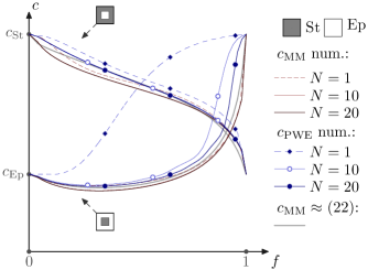
Figure 1: Effective speed $c$ versus concentration $f$ of square rods for 2D St/Ep and Ep/St lattices (see details in the text).

Step 1. Calculate the multiplicative integral (28)₂ defining $\mathbf{M}_{0}$. For an arbitrary $\mu(\mathbf{x})$, one way is to use a discretization scheme. Divide the segment $x_{1}\in[0,1]$ into $N_{1}$ intervals $[x_{1}^{(i)},x_{1}^{(i+1)})\equiv\Delta_{i}$, $i=1..N_{1}$, of small enough length. Calculate $2N+1$ Fourier coefficients $\widehat{\mu}_{n}(x_{1}^{(i)})$, $n=-N..N$ and the $(2N+1)\times(2N+1)$ matrices $\mathbf{Q}_{0}(x_{1}^{(i)})$ for each $i=1..N_{1},$ and then use the approximate formula $\mathbf{M}_{0}=\prod_{i=N_{1}}^{1}\exp\left[\Delta_{i}\mathbf{Q}_{0}(x_{1}^{(i)})\right]$. Recall that $\widehat{\int}$ satisfies the chain rule and is exactly equal to $\exp(\Delta_{i}\mathbf{Q}_{0})$ for $x_{1}\in\Delta_{i}$ if $\mu(\mathbf{x})$ does not depend on $x_{1}$ within $\Delta_{i}$. Therefore the calculation is much simpler in the common case of a piecewise homogeneous unit cell with only a few inclusions of simple shape (see the example below).

Step 2. Solve the system $(\mathbf{M}_{0}-\mathbf{I})\mathbf{w}_{\widehat{1}}=i\mathbf{w}_{\widehat{0}}$ for unknown $\mathbf{w}_{\widehat{1}}$. First remove one zero row and one zero column in the matrix $\mathbf{M}_{0}-\mathbf{I}$ (see the remark below (10)). Then the vector $\mathbf{w}_{\widehat{1}}$ is uniquely defined and may be found by any standard method. Note that only a single component of $\mathbf{h}$ is needed to evaluate $\widetilde{\mathbf{w}}_{\widehat{0}}\cdot\mathbf{w}_{\widehat{1}}\mathbf{.}$ Finally dividing by $\langle\rho\rangle$ yields the desired result (28)₁.

As an example, we calculate the effective shear-wave speed $c$ versus the volume fraction $f$ of square rods periodically embedded in a matrix material forming a 2D square lattice with translations parallel to the inclusion edges. A high-contrast pair of materials is chosen such as steel ($\equiv$ St, with $\rho=7.8\ 10^{3}\$kg/m³, $\mu=80\$GPa) and epoxy ($\equiv$ Ep, with $\rho=1.14\ 10^{3}\$kg/m³, $\mu=1.48\$GPa). We consider two conjugated St/Ep and Ep/St configurations, where the matrix and rod materials are either St and Ep or Ep and St, respectively. The results are displayed in Fig. 1. The curves $c_{\mathrm{MM}}(f)$ are computed by the present monodromy-matrix (MM) method, Eq. (28)₁, they are complemented by the approximation (22). Also shown for comparison are the curves $c_{\mathrm{PWE}}(f)$ computed from the truncated formulaKAG of the conventional PWE method based on a 2D Fourier transform of (3). Calculations are performed for a different fixed number $2N+1\equiv d$ of the 1D Fourier coefficients of $\mu(\mathbf{x})$, which implies $2d\times 2d$ monodromy matrix in (28)₁ and, by contrast, $d^{2}\times d^{2}$ matrix in the PWE formulaKAG . Apart from this advantage of the MM calculation, it is also seen to be remarkably more stable - with a reasonable fit provided already at $N=1$. The difference between the MM and PWE numerical curves is especially notable for the case of densely packed steel rods. Interestingly, the MM computation and estimate both predict a steep fall for $c\left(f\right)$ when a small concentration $1-f$ of epoxy forms a ’quasi-insulating network’. The PWE fails to capture this important physical feature for reasons described next.

The far superior stability and accuracy of the MM method observed in Fig. 1 can be explained as follows. The PWE formulaKAG implies calculating $M_{11}\approx\sum_{\left|\mathbf{g}\right|<d}B_{\mathbf{g}}\left|\mathbf{g}\right|^{-2}\left(\left|g_{2}\right|+1\right)^{-2}+O\left(d^{-1}\right)$ with bounded coefficients $B_{\mathbf{g}},$ where $\mathbf{g}$ are the 2D reciprocal lattice vectors (we use here that the components of the vector $\widehat{\partial_{1}\mu}$ for piecewise constant $\mu(\mathbf{x})$ are of order $\left(\left|g_{2}\right|+1\right)^{-1},$ and that the matrix corresponding to ${\mathcal{C}}_{0}^{-1}$ is close to diagonally-dominant and hence its eigenvalues are of order $\left|\mathbf{g}\right|^{-2}$). Thus the accuracy of the PWE method is expected to be of order $d^{-1}.$ In contrast, the accuracy of the MM method, where the 1D Fourier expansion is performed inside a multiplicative integral that is ’close’ to exponential, is expected to be on the order $e^{-d}.$ This can be understood from the MM equation (28)₁ where the $2d\times 2d$ matrix $(\mathbf{M}_{0}-\mathbf{I})^{-1}$ can be replaced by $2(\mathbf{M}_{0}-\mathbf{M}_{0}^{-1})^{-1}$ with eigenvalues of order $e^{-n},~{}n=1..d$.

Acknowledgement. This work has been supported by the grant ANR-08-BLAN-0101-01 and the project SAMM. A.N.N. acknowledges support from the CNRS.

References

(1) D. Torrent, A. Håkansson, F. Cervera, and J. Sánchez-Dehesa,
Phys. Rev. Lett. 96, 204302 (2006); D. Torrent, J. Sánchez-Dehesa,
Phys. Rev. B 74, 224305 (2006); J. Phys. 9, 323 (2007);
ibid. 10, 023004 (2008).
(2) J. Mei, Z. Liu, W. Wen, P. Sheng,
Phys. Rev. Lett. 96, 024301 (2006);
Phys. Rev. B 76, 134205 (2007).
(3) J.O. Vasseur, P.A. Deymier, B. Djafari-Rouhani, Y. Pennec,
A.-C. Hladky-Hennion,
Phys. Rev. B 77, 085415 (2008); Y. Pennec, J.O. Vasseur,B.
Djafari-Rouhani, L. Dobrzynski, P.A. Deymier, Surf. Sci. Rep.
65, 229-291 (2010).
(4) A. A. Krokhin, J. Arriaga, L. N. Gumen, Phys. Rev. Lett.
91, 264302 (2003).
(5) Q. Ni and J. Cheng, J. Appl. Phys. 101, 073515 (2007).
(6) A. A. Kutsenko, A. L. Shuvalov, A. N. Norris, O. Poncelet,
submitted.
(7) I.V. Andrianov, J. Awrejcewicz, V.V. Danishevs’kyy, D.
Weichert, J. Comput. Nonlinear Dynam. 6, 011015
(2011)