The origin of dark matter, matter-anti-matter asymmetry, and inflation
Abstract
A rapid phase of accelerated expansion in the early universe, known as inflation, dilutes all matter except the vacuum induced quantum fluctuations. These are responsible for seeding the initial perturbations in the baryonic matter, the non-baryonic dark matter and the observed temperature anisotropy in the cosmic microwave background (CMB) radiation. To explain the universe observed today, the end of inflation must also excite a thermal bath filled with baryons, an amount of baryon asymmetry, and dark matter. We review the current understanding of inflation, dark matter, mechanisms for generating matter-anti-matter asymmetry, and the prospects for testing them at ground and space based experiments.
I Introduction
This review aims at building a consistent picture of the early universe where the three pillars of modern cosmology: inflation, baryogenesis and the synthesis of dark matter can be understood in a testable framework of physics beyond the Standard Model (SM).
Inflation Guth (1981), which is a rapid phase of accelerated expansion of space, is the leading model that explains the origin of matter; during this phase, primordial density perturbations are also stretched from sub-Hubble to super-Hubble length scales Mukhanov et al. (1992). A strong support for such an inflationary scenario comes from the precision measurement of these perturbations in the cosmic microwave background (CMB) radiation, e.g. by the Cosmic Background Explorer (COBE) Smoot et al. (1992) and the Wilkinson Microwave Anisotropy Probe (WMAP) Komatsu et al. (2011) satellites. However, one of the most serious challenges faced by inflationary models is that only a few of them provide clear predictions for crucial questions regarding the nature of the matter created after inflation and the mode of exiting inflation in a vacuum that can excite the SM degrees of freedom (d.o.f) Mazumdar and Rocher (2011).
From observations we know that the current universe contains atoms, non-relativistic, non-luminous dark matter, and the rest in the form of dark energy. While some billion years ago it was atoms, photons and neutrinos, and non-relativistic dark matter Komatsu et al. (2011). Therefore, it is mandatory that the inflationary vacuum must excite these SM baryons, and create the right abundance of dark matter. Since the success of Big Bang Nucleosynthesis (BBN) Iocco et al. (2009) requires an asymmetry between the baryons and anti-baryons of order one part in , it is necessary that the baryonic asymmetry must have been created dynamically in the early universe before the BBN Sakharov (1967).
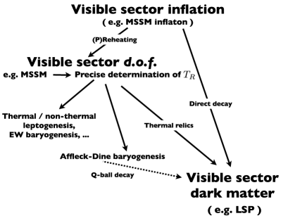
The prime question is what sort of visible sector beyond the SM would accomplish all these goals – inflation, matter creation, and seed perturbations for the CMB. Beyond the scale of electroweak SM (at energies above GeV) there are plethora of candidates, e.g. Bustamante et al. (2009). However the low scale supersymmetry (SUSY) provides an excellent platform, which have been built on the success of the electroweak physics Nilles (1984); Haber and Kane (1985); Martin (1997); Chung et al. (2005). The minimal supersymmetric extension of the SM, known as MSSM, or its minimal extensions, provides many testable imprints at the collider experiment Nath et al. (2010). In particular, the lightest SUSY particle (LSP) can be electrically neutral, and will be an ideal candidate for the weakly interacting massive particle (WIMP) as a dark matter Goldberg (1983); Ellis et al. (1984a), whose abundance can now be calculated from the direct decay of the inflaton, or from the decay products of the inflaton, as shown in Fig. 1.
If such a visible sector, with the known gauge interactions, can also provide us with an inflationary potential capable of matching the current CMB data, then we would be able to identify the origin of the inflaton, its mass and couplings, and the vacuum energy density within a testable theory, such as the MSSM. The inflaton’s gauge invariant couplings would enable us to ascertain the post-inflationary dynamics, and the exact mechanism for particle creation from the inflaton’s coherent oscillations, known as (p)reheating Allahverdi et al. (2010a). We would be able to precisely determine the largest reheat temperature, , of the post-inflationary universe, during which all the MSSM d.o.f come in chemical and in kinetic equilibrium for the first time ever. Once the relevant d.o.f are created it would be possible to build a coherent picture where we will be able to understand the origin of baryogenesis and the dark matter in a consistent framework as illustrated in Fig. 1.
This review is divided into three parts. In the first part we will discuss the origin of inflation, and how to connect the models of inflation to the current CMB observations. We will keep our discussions general and provide some examples of non-SUSY models of inflation. We will mainly focus on SUSY based models and its generalization to supergravity (SUGRA). We will discuss the epoch of reheating, preheating and thermalization for an MSSM based models of inflation. In the second part of the review, we will focus on baryogenesis. We will state the conditions for generating baryogenesis. We will discuss electroweak baryogenesis, baryogenesis induced by lepton asymmetry, known as leptogenesis, and the MSSM based Afflck-Dine baryogenesis which can create non-topological solitons, known as Q-balls. In the third part, we will consider general properties of dark matter, various mechanisms for creating them, some well motivated candidates, and link the origin of dark matter to the origin of inflation within SUSY. We will briefly discuss the ongoing searches of WIMP as a dark matter candidate.
II Particle physics origin of inflation
There are two classes of models of inflation, which have been discussed extensively in the literature, e.g. see reviews Lyth and Riotto (1999); Mazumdar and Rocher (2011). In the first class, the inflaton field belongs to the hidden sector (not charged under the SM gauge group). The direction along which the inflaton field rolls belongs to an absolute gauge singlet, whose couplings to the visible sector – such as that of the SM or MSSM fields are not determined a-priori. A singlet inflaton would couple to the visible and hidden sectors without any biased – such as the case of gravity which is a true singlet, and a color and flavor blind. In the second class, the inflaton candidate distinctly belongs to the visible sector, where the inflaton is charged under the SM or its minimal extension beyond the SM gauge group. This has many advantages, which we will discuss in some details.
Any inflationary models are required to be tested by the amplitude of the density perturbations for the observed large scale structures Mukhanov et al. (1992). Therefore the predictions for the CMB fluctuations are the most important ones to judge the merits of the models, which would contain information about the power spectrum, the tilt in the spectrum, running in the tilt, and tensor to scalar ratio. These observable quantities can be recast in terms of the properties of the potential which we will discuss below. From the particle origin point of view, one of the successful criteria is to end inflation in the right vacuum - where the SM baryons are excited naturally for a successful baryogenesis before BBN Mazumdar and Rocher (2011).
II.1 Properties of inflation
The inflaton direction which leads to a graceful exit needs to be flat with a non-negligible slope provided by a potential which dominates the energy density of the universe. A completely flat potential, or a false vacuum with a very tiny tunneling rate to a lower vacuum, would render inflation future eternal, but not past Borde and Vilenkin (1994); Borde et al. (2003); Linde (1986, 1983); Linde et al. (1996, 1994). A past eternal inflation is possible only if the null geodesics are past complete Biswas et al. (2010, 2006). The slow-roll inflation assumes that the potential dominates over the kinetic energy of the inflaton , and , therefore the Friedmann and the Klein-Gordon equations are approximated as:
| (1) | |||||
| (2) |
where prime denotes derivative with respect to . There exists slow-roll conditions, which constrain the shape of the potential, are give by:
| (3) | |||||
| (4) |
These conditions are necessary but not sufficient for inflation. The slow-roll conditions are violated when , and , which marks the end of inflation.
However, there are certain models where this need not be true, for instance in hybrid inflation models Linde (1994), where inflation comes to an end via a phase transition, or in oscillatory models of inflation where slow-roll conditions are satisfied only on average Damour and Mukhanov (1998); Liddle and Mazumdar (1998), or inflation happens in oscillations Biswas and Mazumdar (2009), or in fast roll inflation where the slow-roll conditions are never met Linde (2001). The K-inflation where only the kinetic term dominates where there is no potential at all Armendariz-Picon et al. (1999).
One of the salient features of the slow-roll inflation is that there exists a late time attractor behavior, such that the evolution of a scalar field after sufficient e-foldings become independent of the initial conditions Salopek and Bond (1990).
The number of e-foldings between, , and the end of inflation, , is defined by:
| (5) |
where is defined by , provided inflation comes to an end via a violation of the slow-roll conditions. The number of e-foldings can be related to the Hubble crossing mode by comparing with the present Hubble length . The final result is Liddle and Leach (2003)
| (6) |
where the subscripts () refer to the end of inflation (end of reheating). Today’s Hubble length would correspond to number of e-foldings, whose actual value would depend on the equation of state, i.e. ( denotes the pressure, denotes the energy density), from the end of inflation to radiation and matter dominated epochs. A high scale inflation with a prompt reheating with relativistic species would yield approximately, . A significant modification can take place if the scale of inflation is low Lyth and Stewart (1995, 1996); Mazumdar (1999); Mazumdar and Perez-Lorenzana (2001); Arkani-Hamed et al. (2000); Green and Mazumdar (2002).
II.2 Density Perturbations
II.2.1 Scalar perturbations
Small inhomogeneities in the scalar field, , such that , induce perturbations in the background metric, but the separation between the background metric and a perturbed one is not unique. One needs to choose a gauge. A simple choice would be to fix a gauge where the non-relativistic limit of the full perturbed Einstein equation can be recast as a Poisson equation with a Newtonian gravitational potential, . The induced metric can be written as, e.g. Mukhanov et al. (1992):
| (7) |
Only in the presence of Einstein gravity and when the spatial part of the energy momentum tensor is diagonal, i.e. , it follows that .
During inflation the massless inflaton (with mass squared: ) perturbations, , are stretched outside the Hubble patch. One can track their perturbations from a sub-Hubble to that of a super-Hubble length scales. Right at the time when the wave numbers are crossing the Hubble patch, one finds a solution for as
| (8) |
where denotes the instance of Hubble crossing. One can define a power spectrum for the perturbed scalar field
| (9) |
Note that the phase of can be arbitrary, and therefore, inflation has generated a Gaussian perturbation. Now, one has to calculate the power spectrum for the metric perturbations. For a critical density universe
| (10) |
where . Therefore, one obtains:
| (11) |
where the right hand side can be evaluated at the time of horizon exit . The temperature anisotropy seen by the observer in the matter dominated epoch is proportional to the Newtonian potential, .
Besides tracking the perturbations in the longitudinal gauge with the help of Newtonian potential, there exists another useful gauge known as the comoving gauge. By definition, this choice of gauge requires a comoving hypersurface on which the energy flux vanishes, and the relevant perturbation amplitude is known as the comoving curvature perturbation, Lukash (1980); Mukhanov et al. (1992). For the super-Hubble modes, , the comoving curvature perturbation, is a conserved quantity, and it is proportional to the Newtonian potential, . Therefore, can also be expressed in terms of curvature perturbations Liddle and Lyth (1993, 2000)
| (12) |
and the corresponding power spectrum . With the help of the slow-roll equation , and the critical density formula , one obtains
| (13) |
where we have used the slow-roll parameter . The COBE satellite measured the CMB anisotropy and fixes the normalization of on very large scales. If we assume that the primordial spectrum can be approximated by a power law (ignoring the gravitational waves and the dependence of the power ) Komatsu et al. (2009)
| (14) |
where is called the spectral index (or spectral tilt), the reference scale is: , and the error bar on the normalization is given at , and
| (15) |
It is important to stress that these central values and error bars vary significantly when other parameters are introduced to fit the data, in part because of degeneracies between parameters (in particular with , the optical depth , its running, the tensor-to-scalar ratio, , and the fraction of cosmic strings). The spectral index is defined as
| (16) |
This definition is equivalent to the power law behavior if is close to a constant quantity over a range of of interest. One particular value of interest is . If , the spectrum is flat and known as Harrison-Zeldovich spectrum Harrison (1970); Zeldovich (1970). For , the spectrum is tilted, and () is known as a blue (red) spectrum. In the slow-roll approximation, this tilt can be expressed in terms of the slow-roll parameters and at first order:
| (17) |
where
| (18) |
The running of these parameters are given by Salopek and Bond (1990). Since the slow-roll inflation requires that , therefore naturally predicts small variation in the spectral index within Kosowsky and Turner (1995)
| (19) |
It is possible to extend the calculation of metric perturbation beyond the slow-roll approximations based on a formalism similar to that developed in Refs. Mukhanov (1985); Sasaki (1986); Mukhanov (1989); Kolb et al. (1995).
II.2.2 Multi-field perturbations
Inflation can proceed along many flat directions with many light fields. Their perturbations can be tracked conveniently in a comoving gauge, on large scales remains a good conserved quantity, provided each field follow slow-roll condition. The comoving curvature perturbations can be related to the number of e-foldings, , given by Salopek (1995); Sasaki and Stewart (1996)
| (20) |
where is measured by a comoving observer while passing from flat hypersurface (which defines ) to the comoving hypersurface (which determines ). The repeated indices are summed over and the subscript denotes a component of the inflaton Lyth and Riotto (1999); Lyth and Liddle (2009). If the random fluctuations along have an amplitude , one obtains:
| (21) |
For a single component , and then Eq. (21) reduces to Eq. (II.2.1). By using slow-roll equations we can again define the spectral index
| (22) |
where , and similarly . For a single component we recover Eq. (17) from Eq. (22). In the case of multi-fields, one has to distinguish adiabatic from isocurvature perturbations. Present CMB data rules out pure isocurvature perturbation spectrum Beltran et al. (2004); Komatsu et al. (2009), although a mixture of adiabatic and isocurvature perturbations remains a possibility.
II.2.3 Gravitational waves
During inflation stochastic gravitational waves are expected to be produced similar to the scalar perturbations Grishchuk (1975); Grishchuk and Sidorov (1989); Allen (1988); Sahni (1990). For reviews on gravitational waves, see Mukhanov et al. (1992); Maggiore (2000). The gravitational wave perturbations are described by a line element , where
| (23) |
The gauge invariant and conformally invariant -tensor is symmetric, traceless , and divergenceless ( is a covariant derivative). Massless spin gravitons have two transverse degrees of freedom (d.o.f)
For the Einstein gravity, the gravitational wave equation of motion follows that of a massless Klein Gordon equation Mukhanov et al. (1992). Especially, for a flat universe
| (24) |
As any massless field, the gravitational waves also feel the quantum fluctuations in an expanding background. The spectrum mimics that of Eq. (9)
| (25) |
Note that the spectrum has a Planck mass suppression, which suggests that the amplitude of the gravitational waves is smaller compared to that of the scalar perturbations. Therefore it is usually assumed that their contribution to the CMB anisotropy is small. The corresponding spectral index can be expanded in terms of the slow-roll parameters at first order as
| (26) |
Note that the tensor spectral index is negative. It is expected that PLANCK could detect gravity waves if , however the spectral index will be hard to measure in forthcoming experiments. The primordial gravity waves can be generated for large field value inflationary models. Using the definition of the number of e-foldings it is possible to derive the range of Lyth and Liddle (2009); Lyth (1997); Hotchkiss et al. (2008))
| (27) |
Note that it is possible to get sizable, , for in assisted inflation (discussed below), and in inflection point inflation discussed in Ref. Ben-Dayan and Brustein (2010). If the tensor-to-scalar ratio and/or a running are introduced, the best fit for and error bars (at ) , Komatsu et al. (2009). These data therefore suggest that a red spectrum is favored ( excluded at from WMAP and at when other data sets are included) if there is no running.
II.3 Generic models of inflation
II.3.1 High scale models of inflation
The most general form for the potential of a gauge singlet scalar field contains an infinite number of terms,
| (28) |
The renormalizable terms allows to prevent all terms with . By imposing the parity , under which , allows to prevent all terms with odd. Most phenomenological models of inflation proposed initially assume that one or two terms in Eq. (28) dominate over the others, though some do contain an infinite number of terms.
Power-law chaotic inflation:
The simplest inflation model by the number of free parameters is perhaps the chaotic inflation Linde (1983) with the potential dominated by only one of the terms in the above series
| (29) |
with a positive integer. The first two slow-roll parameters are given by
| (30) |
Inflation ends when , reached for . The largest cosmological scale becomes super-Hubble when , which is super Planckian; this is the first challenge for this class of models. The spectral index for the scalar and tensor to scalar ratio read:
| (31) |
The amplitude of the density perturbations, if normalized at the COBE scale, yields to extremely small coupling constants; (for i.e. ). The smallness of the coupling, , is often considered as an unnatural fine-tuning. Even when dimension full, for example if , the generation (and the stability) of a mass scale, GeV, is a challenge in theories beyond the SM, as they require unnatural cancellations. These class of models have an interesting behavior for initial conditions with a large phase space distribution where there exists a late attractor trajectory leading to an end of inflation when the slow-roll conditions are violated close to the Planck scale Linde (1983, 1985); Brandenberger and Kung (1990); Kofman et al. (2002).
Note that the above mentioned monomial potential can be a good approximation to describe in a certain field range for various models of inflation proposed and motivated from particle physics; natural inflation when the inflaton is a pseudo-Goldstone boson Freese et al. (1990), or the Landau-Ginzburg potential when the inflaton is a Higgs-type field Bezrukov and Shaposhnikov (2008). The necessity of super Planckian VEVs represents though a challenge to such embedding in particle physics and supergravity (SUGRA).
Exponential potential:
An exponential potential also belongs to the large field models:
| (32) |
It would give rise to a power law expansion , so that inflation occurs when . The case corresponds to the exactly de Sitter evolution and a never ending accelerated expansion. Even for , violation of slow-roll never takes place, since and inflation has to be ended by a phase transition or gravitational production of particles Lyth and Riotto (1999); Copeland et al. (2001).
The confrontation to the CMB data yields: and ; the model predicts a hight tensor to scalar ratio and it is within the one sigma contour-plot of WMAP (with non-negligible ) for .
II.3.2 Assisted inflation
Many heavy fields could collectively assist inflation by increasing the effective Hubble friction term for all the individual fields Liddle et al. (1998). This idea can be illustrated with the help of identical scalar fields with an exponential potentials, see Eq. (32), where now , where . For a particular solution; where all the scalar fields are equal: .
| (33) | |||||
| (34) |
These can be mapped to the equations of a model with a single scalar field by the redefinitions , so the expansion rate is , provided that . The expansion becomes quicker the more scalar fields there are. In particular, potentials with , which for a single field are unable to support inflation, can do so as long as there are enough scalar fields to make .
In order to calculate the density perturbation produced in multi-scalar field models, we recall the results from Eq. (21). Since , we have , we yield: .
Note that this last expression only contains one of the scalar fields, chosen arbitrarily to be . The estimation for the spectral tilt is given by : , which matches that produced by a single scalar field with . The more scalar fields there are, the closer to scale-invariance is the spectrum that they produce. The above calculation can be repeated for arbitrary slopes, . In which case the spectral tilt would have been given by , where . The above scenario has been generalized to study arbitrary exponential potentials with couplings, Copeland et al. (1999); Green and Lidsey (2000).
Assisted chaotic inflation:
Multi-scalar fields of chaotic type has interesting properties Jokinen and Mazumdar (2004):
| (35) |
(for ). The chaotic inflation can now be driven at VEVs, , below the Planck scale Kanti and Olive (1999a, b). The effective slow-roll parameters are given by: and , where are the slow-roll parameters for the individual fields. Inflation can now occur for field VEVs Jokinen and Mazumdar (2004):
| (36) |
where is the number of e-foldings. Obviously, all the properties of chaotic inflation can be preserved at VEVs , including the prediction for the tensor to scalar ration for the stochastic gravity waves, i.e. . For and , it is possible to realize a sub-Planckian inflation, the spectral tilt close to the flatness: , and large tensor to scalar ratio, i.e. .
N-flation:
Amongst various realizations of assisted inflation, N-flation is perhaps the most interesting one. The idea is to have number of axions, where is the axion decay constant, of order drive inflation simultaneously with a leading order potential Dimopoulos et al. (2005):
| (37) |
where are axion fields correspond to the partners of Kähler moduli. The ellipses contain higher order contributions. In a certain Type-IIB compactification, it is assumed that all the moduli are heavy and thus stabilized by prior dynamics, including that of the volume modulus. Only the axions of are light Dimopoulos et al. (2005). The assumption of decoupling the dynamics of Kähler modulus from the axions is still a debatable issue, see Kallosh (2008). After rearranging the potential for the axions, and expanding them around their minima for a canonical choice of the kinetic terms, the Lagrangian simplifies to the lowest order in expansion:
| (38) |
The exact calculation of is hard, assuming all of the mass terms to be the same GeV, and , it is possible to match the current observations with a tilt in the spectrum, , and large tensor to scalar ratio: for . There are also realizations of assisted inflation via branes Mazumdar et al. (2001); Cline and Stoica (2005); Becker et al. (2005).
II.3.3 Hybrid inflation
The end of inflation can happen via a waterfall triggered by a Higgs (not necessarily the SM Higgs) field coupled to the inflaton, first discussed in Linde (1991, 1994); Copeland et al. (1994). The model is based on the potential given by Linde (1991, 1994)
| (39) |
where is the inflaton and is the Higgs-type field. and are two positive coupling constants, and are two mass parameters. It is the most general form (omitting a quartic term ) of renormalizable potential satisfying the symmetries: and . Inflation takes place along the valley and ends with a tachyonic instability for the Higgs-type field. The critical point of instability occurs at:
| (40) |
The system then evolves toward its true minimum at , , and .
The inflationary valley, for , where the last e-foldings of inflation is assumed to take. This raises the issue of initial conditions for fields and the fine tuning required to initiate inflation Tetradis (1998); Lazarides and Vlachos (1997); Panagiotakopoulos and Tetradis (1999); Mendes and Liddle (2000); Clesse and Rocher (2008). In Ref. Clesse and Rocher (2008) it was found that when the initial VEV of the inflaton, , a subdominant but non-negligible part of the initial conditions for the phase space leads to a successful inflation, i.e. around less than depending on the model parameters. Initial conditions with super-Planckian VEVs for automatically leads to a successful inflation similarly to chaotic inflation. In the inflationary valley, , the effective potential is given by:
| (41) |
The model predicts a blue tilt in the spectrum, i.e. , in the small field regime, , which is slightly disfavored by the current data.
Two variations of the hybrid inflation idea were proposed assuming that the term is negligible. The two-field scalar potentials are of the form:
| (42) |
They share the common feature of having an inflationary trajectory during which is varying and not vanishing. For , the model is known as Mutated hybrid Stewart (1995b), and corresponds to Smooth hybrid inflation Lazarides and Panagiotakopoulos (1995). The latter involves non-renormalizable terms of order to keep the potential bounded from below.
The potential is valid in the large field limit , since in the small field limit, the potential is not bounded from below and should be completed. For mutated, the model predicts a red spectral index and negligible tensor to scalar ratio, , and , if we assume . For smooth, the end of slow-roll inflation happens by a violation of the conditions; , since no waterfall transition takes place. This allows the predictions for the spectral index to be Lazarides and Panagiotakopoulos (1995), and the ratio for tensor to scalar is found to be negligible.
II.3.4 Inflection point inflation
One of the challenges for inflation is to realize inflation at low scales, preferably below , with the right tilt and the amplitude of the power spectrum. Inflection point inflation admits a large amount of flexibility in the field space – similar to the analogy of a ball rolling on an elastic surface following the least action principle. With the help of two independent parameters, and , it is possible to obtain a large range of tilt in the spectrum, while keeping the amplitude of the perturbations intact. Let us consider a simple realization of such a potential:
| (43) |
where in order to obtain a point of inflection suitable for inflation. The VEV at which inflation occurs is intimately related to the two independent parameters and can happen at wide ranging scales below , and for wide ranging values of .
Here we will generalize this potential to any generic potential which can be written in the following form (here denotes differentiation with respect to ) Enqvist et al. (2010a); Hotchkiss et al. (2011):
| (44) |
where , which is the Taylor expansion, truncated at , around a reference point , which we choose to be the point of inflection where , or saddle point where . The higher order terms in Eq. (44) can be neglected during inflation, provided that
| (45) |
where corresponds to the field value at the end of inflation. Assuming that the slow-roll parameters are small in the vicinity of the inflection point , and that the velocity is negligible, the potential energy gives rise to a period of inflation.
Inflation ends at the point where . By solving the equation of motion, the number of e-foldings of inflation during the slow-roll motion of the inflaton from to , where , is found to be Enqvist et al. (2010a)
| (46) |
It useful to define the parameters and . Note that is the square root of the slow-roll parameter at the point of inflection. The slow-roll parameters can then be recast in the following form:
| (47) | |||||
| (48) | |||||
| (49) |
where . One can solve Eqs. (47-49), for , and in terms of the slow-roll. The equations are non-linear and in general cannot be solved analytically. However, since , , one can find a closed form solution provided that GeV and Allahverdi et al. (2007c); Bueno Sanchez et al. (2007); Enqvist et al. (2010a); Hotchkiss et al. (2011):
| (50) | |||||
| (51) | |||||
| (52) |
One can derive the properties of a saddle point inflation provided , and . The model favors the current observations by matching the COBE normalization and the spectral tilt ranging from . For instance, the lowest value corresponds to the saddle point inflation for .
II.4 Supersymmetric models
One of the most compelling virtues of SUSY is that it can protect the quadratically divergent contributions to the scalar mass, which arise in one-loop computation from the fermion contribution and quartic self interaction of the scalar field. Such corrections generically spoil the flatness of the inflaton potential. The quadratic divergence is independent of the mass of the scalar field and cancel, exactly if , where is the fermion Yukawa and is the quartic scalar coupling. However this procedure fails at 2-loops and one requires fine tuning of the couplings order by order in perturbation theory. In the case of the SM Higgs, a precision of roughly one part in is required in couplings to maintain the Higgs potential, often known as the hierarchy problem or the naturalness problem. The electroweak symmetry is still broken by the Higgs mechanism, but the quadratic divergences in the scalar sector are absent. In the SUSY limit the fermion and scalar masses are degenerate, but the SUSY has to be broken softly at the TeV scale in such a way that it does not spoil the solution to the hierarchy problem, see Nilles (1984); Haber and Kane (1985); Martin (1997); Chung et al. (2005).
The matter fields for SUSY are chiral superfields , which describe a scalar , a fermion and a scalar auxiliary field . The SUSY scalar potential is the sum of the - and -terms:
| (53) |
where is the superpotential, and transforms under a gauge group with the generators of the Lie algebra given by . Note that all the kinetic energy terms are included in the -terms. For inflation, the effects of supergravity (SUGRA) becomes important. At tree level, SUGRA potential is given by the sum of and -terms, see Nilles (1984)
| (54) | |||
| (55) |
where we have added the Fayet-Iliopoulos contribution to the -term, and , where is gauge coupling. Here is the Kähler potential, which is a function of the fields , and . In the simplest case, at tree-level (and ). In general the Kähler potential can be expanded as: . The kinetic terms for the scalars take the form:
| (56) |
The real part of the gauge kinetic function matrix is given by . In general, . The gauginos masses are typically given by . For a universal gaugino masses, are the same for all the three gauge groups of MSSM. In the simplest case, it is just a constant, , and the kinetic terms for the gauge potentials, , are given by:
| (57) |
SUGRA will be broken if one or more of the obtain a VEV. The gravitino, spin component of the graviton, then absorb the Goldstino component to become massive. Requiring classically , as a constraint to obtain the zero cosmological constant, one obtains
| (58) |
II.4.1 F-term inflation
The most well-known model of SUSY inflation driven by -terms is of the hybrid type and based on the superpotential Copeland et al. (1994); Dvali et al. (1994); Linde and Riotto (1997)
| (59) |
where, is an absolute gauge singlet, while and are two distinct superfields belonging to complex conjugate representation, and is an arbitrary constant fixed by the CMB observations. It is desirable to obtain an effective singlet superfield arising from a higher gauge theory such as GUT Langacker (1981), however to our knowledge it has not been possible to implement this idea, see the discussion in Mazumdar and Rocher (2011). Typically would have other (self)couplings which would effectively ruin the flatness required for hybrid inflation.
This form of potential is protected from additional destabilizing contributions with higher power of , if , and carrying respectively the charges , and under R-parity. Then carries a charge so that the action is invariant.
The tree level scalar potential derived from Eq. (59) reads
| (60) |
where we have denoted by the scalar components of . Note the similarity between Eq. (39) and Eq. (60), where , and both and are replaced by only . We will also assume along this direction, and the kinetic terms for the superfields are minimal, i.e. with a kähler potential: .
Let us define two effective real scalar fields canonically normalized, , and , the overall potential can then be recast as:
| (61) |
The global minimum of the potential is located at , . At large VEVs, , the potential also possesses a local valley of minima (at ) in which the field , now rolls on with . This non-vanishing value of the potential both sustain the inflationary dynamics and induces a SUSY breaking.
This induces a splitting in the mass of the fermionic and bosonic components of the superfields and , with and . Note that this description is valid only as long as is sufficiently slow-rolling such that can be considered as a mass term. Therefore radiative corrections do not exactly cancel out Dvali et al. (1994); Lazarides (2000), and provide a one-loop potential which can be calculated by using the Coleman-Weinberg formula Coleman and Weinberg (1973),
| (62) |
where is now the renormalized potential, is the renormalization mass scale. The sum extends over all helicity states , is the fermion number, and is the mass of the i-th state. One obtains:
| (63) |
where , represents a non-physical energy scale of renormalization and denotes the dimensionality. Note that the perturbative approach of Coleman and Weinberg breaks down when close to the inflection point at . For small coupling , the slow-roll conditions (for ) are violated infinitely close to the critical point, , which ends inflation.
The normalization to COBE allows to fix the scale as a function of . If the breaking of does not produce cosmic strings, the contribution to the quadrupole anisotropy simply comes from the inflationary contribution (see Eq. (II.2.1)) and the observed value can be obtained even with a coupling close to unity Dvali et al. (1994). Small values of can render the scale of inflation very low, as low as the TeV scale Randall et al. (1996); Randall and Thomas (1995); Bastero-Gil and King (1998); Bastero-Gil et al. (2003).
However it has been shown that the formation of cosmic strings at the end of -term inflation is highly probable when the model is embedded in SUSY GUTs Jeannerot et al. (2003). In this case, the normalization to COBE receives two contributions, one from inflation and other from cosmic strings Jeannerot (1997); Rocher and Sakellariadou (2005a), which affects the relation at large , and imposes new stringent bounds on GeV, and Rocher and Sakellariadou (2005b); Jeannerot and Postma (2005)
| (64) |
by demanding that the cosmic strings cam at best contribute less than of isocurvature fluctuations Bevis et al. (2008). Once is fixed, the spectral index can be computed as the range is found to be: whether cosmic strings form or not Senoguz and Shafi (2003); Jeannerot and Postma (2005), and by including the soft-SUSY breaking terms within minimal kinetic terms in the Kähler potential, the spectral index can be brought down to Rehman et al. (2009).
II.4.2 SUGRA corrections and solutions
For inflaton VEVs below the Planck scale, the SUGRA effects can become important and may ruin the flatness of the potential. The SUGRA potential is now given by Eq. (II.4), where the -terms containing an additional exponential factor. Various cross terms between the Kähler and the superpotential leads to the soft breaking mass term for the light scalar fields Dine et al. (1984); Bertolami and Ross (1987); Copeland et al. (1994); Dine et al. (1996b, 1995b); Linde and Riotto (1997)
| (65) |
where GeV contains soft-SUSY breaking mass term for the low scale SUSY breaking scenarios. Once the inflaton gets a mass , the contribution to the second slow-roll parameter becomes order unity and the slow roll inflation ends, i.e. . This is known as the SUGRA- problem.
When there are more than one chiral superfields, as in the -term hybrid model, it can be possible to cancel the dominant correction to the inflaton mass by choosing an appropriate Kähler term Stewart (1995a); Copeland et al. (1994). For non-minimal Kähler potentials, such as
| (66) |
the kinetic terms are non-minimal because . One obtains: One again obtains a problematic contribution to the inflaton mass, i.e. . Several mechanisms have been proposed to tackle this -problem. One can impose, , which is sufficient to keep the slow roll inflation safe, but without much physical motivation. For a generic inflationary model it is not possible to compute at all.
Shift and Heisenberg symmetry:
Safe non-minimal Kähler potentials have also been proposed Brax and Martin (2005); Antusch et al. (2009b); Pallis (2009); Bastero-Gil and King (1999) making use of the shift symmetry. Under this symmetry, a superfield , where is a constant. Kawasaki et al. (2000, 2001) to protect the Kähler potential of the form . This symmetry generates an exactly flat direction for an inflaton field and a non-invariance of the superpotential induces some slope to its potential to allow slow-roll at the loop level. Another symmetry - the Heisenberg symmetry - has also been invoked to protect the form of the Kähler potential Antusch et al. (2009a), where the effective Kähler is a no-scale type of the form . This solves the SUGRA--problem by canceling the exponential term . However note that Kähler potentials generically obtains quantum corrections unlike the non-renormalization theorem which can only protect the superpotential terms Grisaru et al. (1979). Such corrections are hard to compute without knowing the ultra-violet completion, and the exact matter sector for the inflationary model Berg et al. (2006); Berg et al. (2005a, b). Note that none of these papers considered MSSM matter sector.
Inflection point inflation:
For any smooth potential, it is possible to drive inflation near the saddle point, , or near the point of inflection, . These are special points where the effective mass term of the inflaton vanishes and the potential does not suffer through SUGRA- problem Allahverdi et al. (2006, 2007c); Mazumdar et al. (2011). In the saddle point case the potential can be made so flat that inflation can be driven eternally Allahverdi et al. (2006, 2007d).
From the low-energy perspective, the most generic and dangerous SUGRA corrections to the inflaton potential ( with minimal and non-minimal Kähler potentials for ) would have a large vacuum energy contribution. To complicate further, one may even assume that the flatness of is lifted by non-renormalizable contribution to the potential Mazumdar et al. (2011):
| (67) |
where . As mentioned above the interesting observation is that, in fact, there always exists a range of field values, , for which a full potential admits a point of inflection with all known sources of corrections taken into account. Now, all the uncertainties in the corrections to the Kähler potential can be absorbed in the full potential, such that the flat region admits a slow roll inflation with Mazumdar et al. (2011). The condition for this inflection point is , where we characterize the fine-tuning by defined as:
| (68) |
When is small, a point of inflection exists such that , with
| (69) |
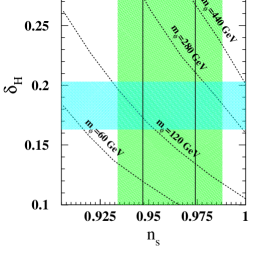
We can Taylor expand the potential about as discussed in section II.3.4, and analyze the CMB constraints as shown in Fig. 2.
II.4.3 D-term inflation
In Refs. Stewart (1995a); Binétruy and Dvali (1996); Halyo (1996), it was noticed that a perfectly flat inflaton potentials can be constructed using a constant contribution coming from the -term. In addition, the SUGRA- problem arising in -term models does not appear for -terms driven inflation because the -sector of the potential does not receive exponential contributions from non-minimal SUGRA. The model however requires the presence of a Fayet-Iliopoulos (FI) term , and therefore a symmetry which generates it. For a Kähler potential , the -terms
(where ) give rise to a scalar potential:
| (70) |
where and are respectively the gauge coupling constants and the generators of each factors of the symmetry of the action, running over all factors of the symmetry, and is the gauge kinetic function. If this symmetry contains a factor , the most general action then allows for the presence of a constant contribution .
The simplest realization of -term inflation reproduces the hybrid potential with three chiral superfields, , , and with non-anomalous (an abelian theory is said to be anomalous if the trace of the generator is non-vanishing ) charges Binétruy and Dvali (1996); Halyo (1996). The superpotential can be written as
| (71) |
In what follows, we assume the minimal structure for (i.e., =1) and take the minimal Kähler potential, i.e. .. Then the scalar potential reads
| (72) |
where is the gauge coupling of . The global minimum of the potential is obtained for and , which is SUSY preserving but induces the breaking of . For the potential is minimized for and therefore, at the tree level, the potential exhibits a flat inflationary valley, with vacuum energy .
The radiative corrections depend on the splitting between the effective masses of the components of the superfields and , because of the transient -term SUSY breaking. The radiative corrections are given by the Coleman-Weinberg expression Coleman and Weinberg (1973) and the full potential inside the inflationary valley reads
| (73) |
with . Inflation ends when the slow-roll conditions break down, that is for , and the predictions for the inflationary parameters are very similar to the previous discussion on -term inflation.
II.5 MSSM flat direction inflation
So far we have discussed inflationary models where the inflaton sector belongs to the hidden sector (not charged under the SM gauge group), such models will have at least one SM gauge singlet component, whose couplings to other fields and mass are chosen just to match the CMB observations. These models are simple but lack proper embedding within MSSM or its minimal extensions.
In order to construct a predictable hidden sector model of inflation, one must know all the inflaton couplings to the hidden and visible matter. One such unique model has been constructed within type IIB string theory, where it was found that all the inflaton energy is transferred to exciting the hidden matter Cicoli and Mazumdar (2010b, a), and the universe could be prematurely dominated by the hidden sector dark matter. Such obstacles do not arise if the last phase of inflation occurs within MSSM.
II.5.1 Introducing MSSM and its flat directions
In addition to the usual quark and lepton superfields, MSSM has two Higgs fields, and . Two Higgses are needed because is forbidden in the superpotential. The superpotential for the MSSM is given by, see Nilles (1984); Haber and Kane (1985); Martin (1997); Chung et al. (2005)
| (74) |
where in Eq. (74) are chiral superfields, and the dimensionless Yukawa couplings are matrices in the family space. We have suppressed the gauge and family indices. The fields are doublets, while are singlets. The last term is the term, which is a SUSY version of the SM Higgs boson mass. Terms proportional to or are forbidden in the superpotential, since must be analytic in the chiral fields. and are required not only because they give masses to all the quarks and leptons, but also for the cancellation of gauge anomalies. The Yukawa matrices determine the masses and CKM mixing angles of the ordinary quarks and leptons through the neutral components of and . Since the top quark, bottom quark and tau lepton are the heaviest fermions in the SM, we assume that only the third family, element of the matrices are important.
The term provides masses to the Higgsinos
| (75) |
and contributes to the Higgs terms in the scalar potential through
| (76) |
Note that Eq. (76) is positive definite. Therefore, it cannot lead to electroweak symmetry breaking without including SUSY breaking soft terms for the Higgs fields, which can be negative. Hence, should almost cancel the negative soft term in order to allow for a Higgs VEV of order GeV. That the two different sources of masses should be precisely of same order is a puzzle for which many solutions has been suggested Kim and Nilles (1984); Giudice and Masiero (1988); Casas and Munoz (1993).
Within MSSM one can construct gauge invariant -and -flat directions, for the list of MSSM flat directions see Dine et al. (1996b); Gherghetta et al. (1996). A flat direction can be represented by a composite gauge invariant operator, , formed from the product of chiral superfields making up the flat direction: . The scalar component of the superfield is related to the order parameter through Dine et al. (1996b).
An example of a -and -flat direction is provided by Enqvist and Mazumdar (2003); Dine and Kusenko (2004)
| (77) |
where is a complex field parameterizing the flat direction, or the order parameter, or the AD field. All the other fields are set to zero. In terms of the composite gauge invariant operators, we would write . Note that a flat direction necessarily carries a global quantum number, which corresponds to an invariance of the effective Lagrangian for the order parameter under phase rotation . In the MSSM the global symmetry is . For example, the -direction has .
From Eq. (80) one clearly obtains for all . However there exists a non-zero F-component given by . Since can not be much larger than the electroweak scale TeV, this contribution is of the same order as the soft SUSY breaking masses, which are going to lift the degeneracy. Therefore, following Dine et al. (1996b), one may nevertheless consider to correspond to a F-flat direction. The relevant -terms read
| (78) |
Therefore the direction is also -flat.
II.5.2 Gauge invariant inflatons of MSSM
A simple observation was first made in Allahverdi et al. (2006, 2007e, 2007c), where the inflaton properties are directly related to the soft SUSY breaking mass term and the A-term of the MSSM. Within MSSM, it is possible to lift the flatness of the gauge invariant combinations of squarks and sleptons away from the point of enhanced gauge symmetry by the -term, while maintaining the -flatness.
Squarks and sleptons driven inflation:
Let us consider a non-renormalizable superpotential term Enqvist and Mazumdar (2003); Dine and Kusenko (2004):
| (79) |
Where , while is the phase term is a gauge invariant superfield which contains the flat direction. Within MSSM (with conserved -parity) all the flat directions are lifted by the non-renormalizable operators with Gherghetta et al. (1996). Two distinct directions are: and , up to an overall phase factor they are parameterized by:
| (80) | |||
| (85) |
where () are color indices, and () denote the quark families for , and () are the weak isospin indices and () denote the lepton families for . Both these directions are lifted by non-renormalizable operators Gherghetta et al. (1996),
| (86) |
Rest of the directions within MSSM are lifted by hybrid operators of type, , which does not lead to cosmologically flat potential viable for slow-roll inflation Allahverdi et al. (2006, 2007e, 2008).
The scalar potential along these directions includes softly broken SUSY mass term for and an -term gives rise to a specific potential Allahverdi et al. (2006, 2007e, 2008)
| (87) |
The -term is a positive quantity with dimension of mass. Note that the first and third terms in Eq. (87) are positive definite, while the -term leads to a negative contribution along the directions whenever . The above potential is similar to Eq.(44). It is possible to find a point of inflection, , provided that , where , and at the lowest orders in , we obtain:
| (88) |
In the case of gravity-mediated SUSY breaking scenarios, . Therefore the condition can indeed be satisfied. Inflation occurs within an interval , in the vicinity of the point of inflection, . Within which the slow-roll parameters, . The Hubble expansion rate during inflation is given by
| (89) |
The amplitude of density perturbations (see Eqs. (II.2.1, 50,51) and the scalar spectral index are given by Allahverdi et al. (2006, 2007e); Bueno Sanchez et al. (2007); Allahverdi and Mazumdar (2006a):
| (90) | |||||
| (91) |
where , and . Running in the tilt is very small. In this case the universe thermalizes in to MSSM radiation instantly in less than one Hubble time after the end of inflation Allahverdi et al. (2011b), see the discussion in Sect. II.6.3.
For GeV, there is an apparent fine-tuning in the parameters , which may look unpleasant. However note that this fine tuning between the two MSSM parameters in the ratio is energy dependent and valid only at the scale of inflation at GeV, but at the TeV scale where the soft masses would be measured at the collider there is no apparent fine tuning in the parameters Allahverdi et al. (2010c).
As shown in Sect. II.4.2, see Fig. 2, the SUGRA corrections will ameliorate the tuning down to , virtually addressing any fine tuning required for the success of MSSM inflation. It was shown in Refs. Allahverdi et al. (2007d, 2008), that the inflection point for the MSSM inflaton is an attractor solution, provided there exists a phase of inflation prior of that of the MSSM with e-foldings. Such large e-foldings can be generated within string theory landscape Allahverdi et al. (2007d), or within MSSM Allahverdi et al. (2008).
Renormalizable superpotential:
The left handed neutrinos can be of Dirac type with an appropriate Yukawa coupling. The simplest way to obtain this would be to augment the SM symmetry by, , where is gauged. The relevant superpotential term is
| (92) |
Here , and are superfields containing the RH neutrinos, left-handed (LH) leptons and the Higgs which gives mass to the up-type quarks, respectively. Note that the monomial represents a -flat direction under the , as well as the SM gauge group.
The value of needs to be small, i.e. , in order to explain the light neutrino mass, corresponding to the atmospheric neutrino oscillations detected by Super-Kamiokande experiment. The potential along this direction, after the minimization along the angular direction, is found to be Allahverdi et al. (2007e, b),
| (93) |
For , there exists an inflection point for which , where inflation takes place
| (94) |
The amplitude of density perturbations follows from Eqs. (II.2.1,50,51) Allahverdi et al. (2007e, b).
| (95) |
Here denotes the loop-corrected value of the inflaton mass at the scale in Eqs. (II.5.2,95). The spectral tilt as usual has a range of values Allahverdi et al. (2007e, b).
MSSM Higgses as inflaton:
The MSSM Higgses are another fine example of a visible sector inflaton provided some restrictions are met Chatterjee and Mazumdar (2011). The required superpotential is given by
| (96) |
This is the -term which were considered an ideal candidate to generate the density perturbations Enqvist et al. (2004a, b), but now they can also provide the required vacuum energy to inflate the universe Chatterjee and Mazumdar (2011). The scalar potential along the -flat direction is given by,
| (97) | |||||
where , and , and
| (98) | |||||
| (99) |
For simplicity, we may assume and to be real. This choice is compatible with the experimental constraints, mainly from the Electron Dipole Moment measurements Pospelov and Ritz (2005). The inflection point can be obtained for , for simplicity let us consider the case for , and when the following condition is satisfied, , where is the tuning required to maintain the flatness of the potential. Although, this tuning could be harsh at the inflationary scale, GeV, but the ratio evolves to at the electroweak scale by virtue of running of the renormalization group equations Chatterjee and Mazumdar (2011). The amplitude of the CMB perturbations can be obtained for and , it is possible to obtain a similar plot like Fig. (3) for Higgs mass GeV, which yields the spectral tilt in the range .
II.6 Preheating, reheating, thermalization
Reheating at the end of inflation is an important aspect of inflationary cosmology. Without reheating the universe would be empty of matter, for a review see Allahverdi et al. (2010a). Reheating occurs through coupling of the inflaton field , to the SM matter. Such couplings must be present at least via gravitational interactions. In particular, if the inflaton is a SM gauge singlet, the relevant couplings to SM are: , where is the scale below which all these effective operators are valid, , is the SM Higgs doublet, and are the left and the right handed SM fermions Allahverdi and Mazumdar (2007b).
Similar couplings would arise if is replaced by right handed sneutrinos, axions, moduli, or any other hidden sector field. Being a SM singlet, can as well couple to other hidden sectors, moduli, axions, etc. Since the hidden sectors are largely unknown, it becomes a challenge for a singlet inflaton to decay solely into the SM d.o.f Cicoli and Mazumdar (2010b, a).
After the end of inflation, the inflaton starts coherent oscillations around its minimum. The frequency of oscillations are determined by the frequency of oscillations, . During this epoch the inflaton can decay perturbatively Albrecht et al. (1982); Turner (1983); Dolgov and Kirilova (1990); Kolb and Turner (1988). Averaging over many oscillations results in a pressureless equation of state where vanishes, so that the energy density starts evolving like a matter domination (in a quadratic potential) with (subscript denotes the quantities right after the end of inflation). For potential the coherent oscillations yield an effective equation of state similar to that of a radiation epoch. If represents the total decay width of the inflaton to pairs of fermions. This releases the energy into the thermal bath of relativistic particles when . The energy density of the thermal bath is determined by the reheat temperature , given by:
| (100) |
where denotes the effective relativistic d.o.f in the plasma. However the inflaton decay products need to thermalize, which requires acquiring kinetic and chemical equilibrium.
II.6.1 Non-perturbative particle creation
If the inflaton coupling to the matter field is large, a completely new channel of reheating opens up due to the coherent nature of the inflaton field, proposed by Traschen and Brandenberger (1990); Shtanov et al. (1995); Kofman et al. (1994, 1997), known as preheating. Let us first consider a simple toy model with interaction Lagrangian
| (101) |
where is another scalar field, in a realistic set-up could take the role of the SM Higgs. We can neglect the effect of expansion provided that the time period of preheating is small compared to the Hubble expansion time , this is reasonable in many cases.
The quantum theory of particle production in the external classical inflaton background begins by expanding the quantum field into creation and annihilation operators and as:
| (102) |
where is the momentum. Since the equation of motion for is linear it can be studied simply mode by mode in Fourier space. The mode functions then satisfy:
| (103) |
where is the amplitude of oscillation in . This is the Mathieu equation which is written in the form
| (104) |
where the dimensionless time variable is and a prime now denotes the derivative with respect to . Comparing the coefficients, we find
| (105) |
The growth of the mode function corresponds to particle production Birrell and Davies (1982). It is well known that the above Mathieu equation Eq. (104) has instabilities for certain ranges of :
| (106) |
where is called the Floquet exponent. For small values of , i.e. , resonance occurs in a narrow instability band about , known as a “narrow resonance” band Traschen and Brandenberger (1990). The resonance is much more efficient if Kofman et al. (1994, 1997). In this case, resonance occurs in broad bands, i.e. the bands include all long wavelength modes , known as broad resonance. This can be understood by studying the condition for particle production in the WKB approximation for the evolution of field which is violated. In the WKB approximation: , which is valid as long as the adiabaticity condition
| (107) |
is satisfied. In the above, the effective frequency is given by
| (108) |
By inserting the effective frequency Eq. (108) into the condition Eq. (107) and following some algebra, the adiabaticity condition is violated for momenta
| (109) |
For modes with these values of , the adiabaticity condition breaks down in each oscillation period when is close to zero. The particle number does not increase smoothly, but rather in “bursts” Kofman et al. (1994, 1997).
The above analysis of neglecting the expansion of the universe is self-consistent. However, as discussed in detail in Kofman et al. (1997), the expansion of space can be included. The equation of motion for becomes
| (110) |
The adiabaticity condition is now violated for momenta satisfying:
| (111) |
Note that the expansion of space makes broad resonance more effective since more modes are red-shifted into the instability band as time proceeds. The detailed analysis yields the same expression for the resonance band except for the exact value of the numerical coefficient of the first term on the r.h.s.. Broad parametric resonance ends when .
In principle, it is also possible to excite the fermions non-perturbatively, in spite of the fact that the occupation number of any fixed state cannot be greater than one (because of the Pauli exclusion principle) Greene and Kofman (1999); Baacke et al. (1998); Giudice et al. (1999a); Greene and Kofman (2000); Peloso and Sorbo (2000), and higher spin gravitinos Maroto and Mazumdar (2000); Kallosh et al. (2000a); Giudice et al. (1999b); Nilles et al. (2001c, b); Kallosh et al. (2000b).
Tachyonic prehetaing:
It is possible that effective frequency of certain mode can be negative. For example in a symmetry breaking potential: , for small field values, the effective mass of the fluctuations of is negative and hence a “tachyonic” resonance will occur, as studied in Felder et al. (2001). For small field values, the equation for the fluctuations of is
| (112) |
The modes with grow with an exponent which approaches in the limit . Given initial vacuum amplitudes for the modes at the intial time of the resonance, the field dispersion at a later time will be given by
| (113) |
The growth of the fluctuations modes terminates once the dispersion becomes comparable to the symmetry breaking scale.
Tachyonic preheating also occurs in hybrid inflation models, see Eq. (39). In this case, it is the fluctuations of which have tachyonic form and which grow exponentially Felder et al. (2001). Preheating in hybrid inflation was first studied in Garcia-Bellido and Linde (1998) using the tools of broad parametric resonance.
End of preheating:
In the above analysis we have neglected the back-reaction of the produced and particles on the dynamics. The presence of particles changes the effective mass of the inflaton oscillations. This back-reaction effect is negligible as long as the change in the square mass of the inflaton is smaller than . In the Hartree approximation, the change in the inflaton mass due to particles is given by Kofman et al. (1997). Another important condition is that the energy in the particles should be sub-dominant. Therefore, , It was found that is smaller than the potential energy of the inflaton field at the time as long as the value at the time is larger than , i.e. . This is roughly speaking the same as the condition for the effectiveness of broad resonance Kofman et al. (1997).
II.6.2 Thermalization
Neither the perturbative decay of the inflaton nor the preheating mechanism produce a thermal spectrum of decay products. In a full thermal equilibrium the energy density and the number density of relativistic particles scale as: and , where is the temperature of the thermal bath. Thus, in full equilibrium the average particle energy is given by: , which obeys the scaling, .
Perturbative reheating and thermalization:
If the inflaton decays perturbatively, then right after the inflaton has decayed completely, the energy density of the universe is given by: . From conservation of energy, the number density of decayed particles is: . Hence, perturbative decay results in a dilute plasma that contains a small number of very energetic particles. A local thermal equilibrium requires re-distribution of the energy among different particles, kinetic equilibrium, as well as increasing the total number of particles, chemical equilibrium. Therefore both number-conserving and number-violating reactions must be involved.
The most important processes for kinetic equilibration are scatterings with gauge boson exchange in the -channel. Due to an infrared singularity, these scatterings are very efficient even in a dilute plasma Davidson and Sarkar (2000); Allahverdi and Mazumdar (2006b). Chemical equilibrium is achieved by changing the number of particles in the reheat plasma. In order to reach full equilibrium the total number of particles must increase by a factor of , where and the equilibrium value is: . This can be a very large number, i.e. . It was recognized in Davidson and Sarkar (2000); Allahverdi and Drees (2002), see also Jaikumar and Mazumdar (2004); Allahverdi (2000) that the most relevant processes are scatterings with gauge-boson exchange in the channel. When these scattering become efficient, the number of particles increases very rapidly, and full thermal equilibrium is established shortly after that Enqvist and Sirkka (1993).
Non-perturbative preheating and thermalization:
In this case the occupation numbers of the excited quanta are typically very high after the initial stages of preheating, Once the occupation numbers of the resonant modes become sufficiently large, re-scattering of the fluctuations begins Khlebnikov and Tkachev (1996); Khlebnikov and Tkachev (1997b, a); Micha and Tkachev (2003, 2004) which terminates the phase of exponential growth of the occupation numbers. The evolution of the field fluctuations evolves to a regime of turbulent scaling which is characterized by the spectrum Micha and Tkachev (2003, 2004), which is non-thermal (for a thermal distribution we would expect ). The phase of turbulence ends once most of the energy has been drained from the inflaton field. At this time quantum processes take over and lead to the thermalization of the spectrum.
II.6.3 Calculation of within MSSM
In the case of MSSM inflation, the inflaton couplings to MSSM d.o.f are known Allahverdi et al. (2011b). It is therefore possible to track the thermal history of the universe from the end of inflation. When the MSSM inflaton passes through minimum, i.e. , the entire gauge symmetry gets restored and all the d.o.f associated with the MSSM gauge group become massless, which is known as the point of enhanced gauge symmetry.
These are the massless modes which couple to the inflaton directly, for instance the d.o.f corresponding to , or that of . At VEVs away from the minimum, the same modes become heavy and therefore it is kinematically unfavorable to excite them. The actual process of excitation depends on how strongly the adiabaticity condition for the time dependent vacuum is violated for the inflaton zero mode.
Couplings for LLe inflaton:
Let us illustrate this with flat direction as an inflaton. The inflaton non-zero VEV completely breaks the symmetry. This results in four massive real scalars, whose masses are obtained from the -terms Allahverdi et al. (2011b)
| (114) |
Here are the and gauge couplings respectively, and denote the inflaton, see Eq. (85). The ’s are Goldstone bosons from breakdown of . They are eaten by the Higgs mechanism and give rise to longitudinal components of the electroweak gauge fields. In the unitary gauge, they are completely removed from the spectrum. The particles decay to squarks, the Higgs particles, and the sleptons with the decay rates given by: . Note that the decay rate is proportional to the VEV of the inflaton, which sets the mass of fields. Couplings of the inflaton to the gauge fields are obtained from the flat direction kinetic terms Allahverdi et al. (2011b)
| (115) |
where , where and are the and gauge fields respectively. The gauge fields decay to (s)quarks, Higgs and Higgsino particles, and (s)leptons with the total decay widths: . Couplings of the inflaton to fermions can also be found in a similar way Allahverdi et al. (2011b).
Instant preheating and thermalization:
The fields that are coupled to the inflaton acquire a VEV-dependent mass that varies in time due to the inflaton oscillations. For illustration, we first focus on the scalar, which are produced every time the inflaton goes through zero. The Fourier eigenmodes of have the corresponding energy
| (116) |
where is the bare mass of the field. The growth of the occupation number of mode can be computed exactly for the first zero-crossing, , where the inflaton near the zero-crossing is given by , from the conservation of energy, where is the amplitude of the inflaton oscillations, GeV, where is the inflection point for inflation, Eq. (88). Note that after a few oscillations, , since the expansion rate during the inflaton oscillations is negligible by virtue of GeV and GeV. The total number density of particles thus produced follows
| (117) |
where . This expression corresponds to the asymptotic value and assumes there is no perturbative decay of the produced particles. However, immediately after adiabaticity is restored, , particles decay into lighter particles (i.e. those particles that have no gauge coupling to the inflaton). In the case of inflaton these are the (s)quarks, Higgs(ino), and (s)leptons.
Thus the fraction that is transferred from the inflaton to ’s, and through their prompt decay into relativistic squarks, at every inflaton zero-crossing, can be computed analytically, and they are given by,
| (118) |
The total number of d.o.f coupled to the inflaton is ( from scalars, from gauge fields, and from fermions). Therefore the fraction of the inflaton energy density that is transferred to relativistic quarks and squarks, see Eq. (118), for , has to be multiplied by (1+3+4)=8 Allahverdi et al. (2011b):
| (119) |
Note that this fraction is independent from the amplitude of oscillations. The draining the inflaton energy is quite efficient, nearly of the inflaton energy density gets transferred to the relativistic species – but not all the SM d.o.f are in thermal equilibrium after one oscillation. It takes near about 120 oscillations to reach the full chemical and kinetic equilibrium via processes requiring and interactions. However due to the hierarchy between , this happens within a single Hubble time after the end of inflation. One can estimate the final reheat temperature Allahverdi et al. (2011b)
| (120) |
where and , see Eq. (88).
III Matter-anti-matter asymmetry
If (p)reheating can provide a thermal bath where all the SM quarks and leptons are excited, it is then an important question to ask – why the present day galaxies and intergalactic medium is primarily made up of baryons rather than anti-baryons?
The baryon abundance in the universe is denoted by , which defines the fractional baryon density with respect to the critical energy density of the universe: . The observational uncertainties in the present value of the Hubble constant; are encoded in Kessler et al. (2009). It is useful to write in terms of the baryon and photon number densities
| (121) |
where is the baryon number density and is for anti-baryons. The photon number density is given by . The best present estimation of the baryon density comes from BBN, which is based on SM physics with 3 neutrino species Fields and Sarkar (2006); Cyburt et al. (2008)
| (122) | |||
| (123) |
The observational data on and are consistent with each other and the expectations from the BBN analysis, but both prefer slightly higher value compared to the abundance , which is smaller than and by at least . The abundance is primarily measured in the stellar systems such as globular clusters.
From the acoustic peaks of the CMB the baryon fraction can be deduced. The WMAP data imply or Komatsu et al. (2011). The WMAP data relies on priors and the choice of number of parameters, it is possible to yield baryon abundance as low as Hunt and Sarkar (2010). In spite of systematic uncertainties the WMAP data is consistent with that of theoretical predictions from BBN. The major unresolved problem is the abundance, stellar measurements are inconsistent with both WMAP and BBN data, and this could be an useful probe of new physics at BBN, see for a review Jedamzik and Pospelov (2009).
Often in the literature the baryon asymmetry is given in relation to the entropy density , where measures the effective number of relativistic species which itself a function of temperature. At the present time , while during BBN , rising up to at GeV. In the presence of supersymmetry at GeV, the number of effective relativistic species are nearly doubled to . The baryon asymmetry defined as the difference of baryon and anti-baryon number densities relative to the entropy density, is bounded by
| (124) |
at , where the numbers are CMB Komatsu et al. (2011), and BBN bounds Fields and Sarkar (2006); Cyburt et al. (2008), respectively.
If at the beginning , then the origin of this small number can not be understood in a CPT invariant universe by a mere thermal decoupling of nucleons and anti-nucleons at MeV. The resulting asymmetry would be too small by at least nine orders of magnitude, see Kolb and Turner (1988). Therefore it is important to seek mechanisms for generating baryon asymmetry, for reviews see Rubakov and Shaposhnikov (1996); Riotto (1998); Dine and Kusenko (2004).
III.1 Requirements for baryogenesis
As pointed out first by Sakharov Sakharov (1967), baryogenesis requires three ingredients: baryon number non-conservation, and violation, and out-of-equilibrium condition. All these conditions are believed to be met in the very early universe.
Baryon number non-conservation:
In the SM, baryon number is violated by non-perturbative instanton processes ’t Hooft (1976b, a). Due to chiral anomalies both baryon number and lepton number currents are not conserved Adler (1969); Bell and Jackiw (1969). However the anomalous divergences come with an equal amplitude and an opposite sign. Therefore remains conserved, while may change via processes which interpolate between the multiple non-Abelian vacua of . The probability for the violating transition is however exponentially suppressed ’t Hooft (1976b, a), but at finite temperatures when , baryon violating transitions are in fact copious Manton (1983).
The violation also leads to proton decay in GUTs Langacker (1981). The dimension operator generates observable proton decay unless GeV. In the MSSM the bound is GeV because the decay can take place via a dimension operator. In the MSSM superpotential there are also terms which can lead to and . Similarly there are other processes such as neutron-anti-neutron oscillations in SM and in SUSY theories which lead to and transitions. These operators are constrained by the measurements of the proton lifetime, which yield the bound years Nakamura et al. (2010).
and violation:
The maximum violation occurs in weak interactions while neutral Kaon is an example of violation in the quark sector which has a relative strength Nakamura et al. (2010). violation is also expected to be found in the neutrino sector. Beyond the SM there are many sources for violation. An example is the axion proposed for solving the strong problem in Peccei and Quinn (1977b, a).
Departure from thermal equilibrium:
If -violating processes are in thermal equilibrium, the inverse processes will wash out the pre-existing asymmetry Weinberg (1979). This is a consequence of -matrix unitarity and -theorem. However there are several ways of obtaining an out-of-equilibrium process in the early universe. Departure from a thermal equilibrium cannot be achieved by mere particle physics considerations but is coupled to the dynamical evolution of the universe.
Out-of-equilibrium decay or scattering:
The condition for out-of-equilibrium decay or scattering is that the rate of interaction must be smaller than the expansion rate of the universe, i.e. . The universe in a thermal equilibrium can not produce any asymmetry, rather it tries to equilibrate any pre-existing asymmetry.
Phase transitions:
They are ubiquitous in the early universe. The transition could be of first, or of second (or of still higher) order. First order transitions proceed by barrier penetration and subsequent bubble nucleation resulting in a temporary departure from equilibrium. The QCD and possibly electroweak phase transitions are examples of first order phase transitions. The nature and details of QCD phase transition is still an open debate Rajagopal and Wilczek (1993); Karsch et al. (2001). Second order phase transitions have no barrier between the symmetric and the broken phase. They are continuous and equilibrium is maintained throughout the transition.
Non-adiabatic motion of a scalar field:
Any complex scalar field carries and , but the symmetries can be broken by terms in the Lagrangian. This can lead to a non-trivial trajectory of a complex scalar field in the phase space. If a coherent scalar field is trapped in a local minimum of the potential and if the shape of the potential changes to become a maximum, then the field may not have enough time to readjust with the potential and may experience completely non-adiabatic motion. This is similar to a second order phase transition but it is the non-adiabatic classical motion which prevails over the quantum fluctuations, and therefore, departure from equilibrium can be achieved. If the field condensate carries a global charge such as the baryon number, the motion can charge up the condensate. This is the basis for the Affleck-Dine baryogenesis Affleck and Dine (1985).
III.2 Sphalerons
At finite temperatures violation in the SM can be large due to sphaleron transitions between degenerate gauge vacua with different Chern-Simons numbers Manton (1983); Klinkhamer and Manton (1984). Thermal scattering produces sphalerons which in effect decay in non-conserving ways below GeV Bochkarev and Shaposhnikov (1987), and thus can exponentially wash away asymmetry. The three important ingredients which play important role are following.
Chiral anomalies:
In the SM there is classical conservation of the baryon and lepton number currents and , but because of chiral anomaly (at the quantum level) the currents are not conserved Adler (1969); Bell and Jackiw (1969). Instead ’t Hooft (1976b),
| (125) |
where is the number of generations, and ( and ) are respectively the and gauge couplings (field strengths). Note that at the quantum level is violated, but is still conserved.
Gauge theory vacua:
in the gauge group, the vacua are classified by their homotopy class , characterized by the winding number which labels the so called -vacua ’t Hooft (1976a); Polyakov (1977). A gauge invariant quantity is the difference in the winding number (Chern-Simons number)
| (126) |
In the electroweak sector the field density is related to the divergence of current. Therefore a change in reflects a change in the vacuum configuration determined by the difference in winding number
| (127) |
For three generations of SM leptons and quarks the minimal violation is . Note that the proton decay requires , so that despite -violation, proton decay is completely forbidden in the SM. The probability amplitude for tunneling from an vacuum at to an vacuum at can be estimated by the WKB method ’t Hooft (1976a)
| (128) |
The baryon number violation rate is negligible at zero temperature, but as argued at finite temperatures the situation is completely different Manton (1983); Kuzmin et al. (1985).
Thermal tunneling:
below the critical temperature of the electroweak phase transition, the sphaleron rate is exponentially suppressed Carson et al. (1990):
| (129) |
where is the functional determinant which can take the values Dine et al. (1992). Above the critical temperature the rate is however unsuppressed. Since the Chern-Simons number changes at most by , one can estimate from Eq. (126) that . Therefore a typical energy of the sphaleron configuration is given by . At temperatures greater than the critical temperature there is no Boltzmann suppression, so that the thermal energy . This determines the size of the sphaleron: Based on this coherence length scale one can estimate the baryon number violation per volume , and per unit time . On dimensional grounds the transition probability would then be given by
| (130) |
where is a constant which incorporates various uncertainties. However, the process is inherently non-perturbative, and it has been argued that damping of the magnetic field in a plasma suppresses the sphaleron rate by an extra power of Arnold et al. (1997), with the consequence that . Lattice simulations with hard thermal loops also give Moore (1999).
Washing out :
Assuming that in the early universe the SM d.o.f are in equilibrium, the transitions and are equally probable. The ratio of rates for the two transitions is given by , where is the free energy difference between the two vacua. Because of a finite density, there is a net chemical potential . Therefore one obtains Bochkarev and Shaposhnikov (1987)
| (131) |
It then follows that an exponential depletion of due to sphaleron transitions remains active as long as
| (132) |
This result imply that below GeV, the sphaleron transitions can wash out any asymmetry being produced earlier in a time scale . This seems to wreck GUT baryogenesis based on conserving groups such as the minimal .
III.3 Mechanisms for baryogenesis
There are several scenarios for baryogenesis, the main contenders being GUT baryogenesis, electroweak baryogenesis, leptogenesis, and baryogenesis through the decay of a field condensate, or Affleck-Dine baryogenesis. Here we give a brief description of these various alternatives.
III.3.1 GUT-baryogenesis
This model relied on out-of-equilibrium decays of heavy GUT gauge bosons , and , for reviews see Dolgov (1992); Kolb and Turner (1988). The decay rate of the gauge boson goes as , where is the mass of the gauge boson and is the GUT gauge coupling. Assuming that the universe was in thermal equilibrium at the GUT scale, the decay temperature is given by
| (133) |
which is smaller than the gauge boson mass. Thus, at , one expects , and hence the net baryon density is proportional to the photon number density . However below the gauge boson abundances decrease and eventually they go out-of-equilibrium. The net entropy generated due to their decay heats up the universe with a temperature which we denote here by . Let us naively assume that the energy density of the universe at is dominated by the bosons with , and their decay products lead to radiation with an energy density , where for . Equating the expressions for the two energy densities one obtains
| (134) |
Therefore the net baryon number comes out to be
| (135) |
is determined from the relation . Thus,
| (136) |
Uncertainties in and violation are now hidden in , but can be tuned to yield total in many models.
Above we have assumed that the universe is in thermal equilibrium when . This might not be true, since for processes the scattering rate is given by , which becomes smaller than at sufficiently high temperatures. Elastic processes maintain thermal contact typically only up to a maximum temperature GeV, while chemical equilibrium is lost already at GeV Enqvist and Eskola (1990); Elmfors et al. (1994).
III.3.2 Electroweak baryogenesis
A popular baryogenesis candidate is based on the electroweak phase transition, during which one can in principle meet all the Sakharov conditions. There is the sphaleron-induced baryon number violation above the critical temperature, various sources of violation, and an out-of-equilibrium environment if the phase transition is of the first order. In that case bubbles of broken are nucleated into a symmetric background with a Higgs field profile that changes through the bubble wall Kuzmin et al. (1985, 1987).
There are two possible mechanisms which work in different regimes: local and non-local baryogenesis. In the local case both violation and baryon number violation takes place near the bubble wall. This requires the velocity of the bubble wall to be greater than the speed of the sound in the plasma Ambjorn et al. (1990); Turok and Zadrozny (1990, 1991), and the electroweak phase transition to be strongly first order with thin bubble walls.
In the non-local case the bubble wall velocity speed is small compared to the sound speed in the plasma. In this mechanism the fermions, mainly the top quark and the tau-lepton, undergo violating interactions with the bubble wall, which results in a difference in the reflection and the transmission probabilities for the left and right chiral fermions. The net outcome is an overall chiral flux into the unbroken phase from the broken phase. The flux is then converted into baryons via sphaleron transitions inside the unbroken phase. The interactions are taking place in a thermal equilibrium except for the sphaleron transitions, the rate of which is slower than the rate at which the bubble sweeps the space Nelson et al. (1992); Cohen et al. (1993).
For a constant velocity profile of the bubble, , the net baryon asymmetry is generated by:
| (137) |
where is the chemical potential, which determines the tilt in the free energy of the sphaleron transitions, and numerically it is equivalent to: . Here determines the profile of the bubble, and denotes the number of Higgs doublets. The net baryon asymmetry can be calculated by following Eq. (130):
| (138) |
where is the transport time of the scattered fermions off the bubble wall, and . For the maximum wall velocity and a typical: for top quarks, the maximum baryon asymmetry is given by: . The function also takes into account the phase, in the favorable scenario one would expect . The details of the transport equations can be found in Refs. Nelson et al. (1992); Kainulainen et al. (2001).
One great challenge for the electroweak baryogenesis is the smallness of violation in the SM at finite temperatures. It has been pointed out that an additional Higgs doublet McLerran et al. (1991); Turok and Zadrozny (1991) would provide an extra source for violation in the Higgs sector. However, the situation is much improved in the MSSM where there are two Higgs doublets and , and two important sources of violation Ellis et al. (1982). The Higgses couple to the charginos and neutralinos at one loop level leading to a violating contribution. There is also a new source of violation in the mass matrix of the top squarks which can give rise to considerable violation Huet and Nelson (1996).
Bubble nucleation depends on the thermal tunneling rate, and the expansion rate of the universe. The tunneling rate has to overcome the expansion rate in order to have a successful phase transition via bubble nucleation at a given critical temperature . The effective potential for the Higgs at finite temperatures can be computed, which takes the form:
| (139) |
The order parameter is given by the ratio of , which has to be larger than one for first order phase transition. For GeV, one obtains the condition for the sphaleron energy Shaposhnikov (1987); Rubakov and Shaposhnikov (1996)
| (140) |
which implies Bochkarev et al. (1991)
| (141) |
In terms of the Higgs field value at ,
| (142) |
where is gauge coupling of , and . Then the bounds in Eqs. (141) translate to
| (143) |
which implies that the phase transition should be strongly first order in order that sphalerons do not wash away all the produced baryon asymmetry. This result is the main constraint on electroweak baryogenesis.
Lattice studies suggest that in the SM the phase transition is strongly first order only below Higgs mass GeV Kajantie et al. (1996); Rummukainen et al. (1998). Above this scale the transition is just a cross-over. Such a Higgs mass is clearly excluded by the LEP measurements Nakamura et al. (2010), thus excluding electroweak baryogenesis within the SM. However, this opens up a possibility to include new physics beyond the SM.
Electroweak baryogenesis induced by new physics:
it was pointed out that by modifying the SM Higgs self-interactions, especially the cubic term, it is possible to enhance the first order phase transition Anderson and Hall (1992). One such example has been considered in Mohapatra and Zhang (1992); Grojean et al. (2005) where non-renormalizable contribution to the Higgs potential has been considered of type:
| (144) |
where is the SM electroweak Higgs doublet and is the scale of new physics which induces the corrections below the energy scale of TeV. At zero temperature the CP-even scalar state can be expanded in terms of its zero-temperature VEV, GeV, and the physical Higgs boson : .
The finite temperature effects are taken into account by adding a thermal mass to the potential:
| (145) |
where is given in the high-temperature expansion of the one-loop thermal potential:
| (146) |
where and are the and gauge couplings, and is the top Yukawa coupling. Note that there is no trilinear term in the effective potential.
The critical temperature at which the minima and are degenerate is given by
| (147) |
The VEV of the Higgs field at the critical temperature in terms of , and is
| (148) |
From Eqs. (147) and (148), one finds that for any given there is an upper bound on to make sure that the phase transition is always first order (), and there is a lower bound on to make sure that the minimum at is a global minimum (). These two combinations chart out a region where the phase transition is indeed first order:
| (149) |
where GeV. In order to ensure that the thermal mass correction is positive: . For these ranges of the ratio , ensuring a successful sphaleron transition for the Higgs mass GeV. One nice aspect of this model is that the non-renormalizable scale can also be constrained from the precision electroweak observable, which can be tested in near future by the LHC Grojean et al. (2005).
III.3.3 Electroweak baryogenesis in MSSM
In the MSSM the ratio can be increased by virtue of the scalar loops which can make the cubic term in the temperature dependent Higgs potential large; . In particular the right handed stop coupling to the Higgs with a large Yukawa coupling. This leads to a strong first order phase transition – as the ratio of , where determines the order parameter Carena et al. (1996); Laine (1996); Cline et al. (1998); Laine and Rummukainen (1998); Cline et al. (2000).
The finite temperature cubic term is given by: , where the lightest right handed stop mass
| (150) |
where is the stop mixing parameter, is the trilinear term in the MSSM superpotential, and is the soft-SUSY breaking mass parameter for the right-handed stop. The coefficient of the cubic term in the effective potential reads
| (151) |
and can be at least one order of magnitude larger than . The implications for the particle spectrum are:
-
•
A light right-handed stop: .
-
•
A heavy left-handed stop: TeV.
-
•
A light SM-like Higgs: GeV, for .
The present LEP constraint on the lightest -even Higgs mass is GeV Nakamura et al. (2010). Note that within MSSM, the lightest Higgs mass is bounded by: . Hence, even an MSSM-based electroweak baryogenesis may be at the verge of being ruled out.
MSSM also provides new violating complex phases in the Higgsino sector, i.e. , with GeV. The -violating phases are also constrained by the electric dipole moments. To match the observational limit on e cm Regan et al. (2002), one requires first and second generation sfermion masses greater than TeV. while the 2-loop electron dipole moment contribution comes out to be: e cm.
III.3.4 Electroweak baryogenesis beyond MSSM
Some of these problems of MSSM can be resolved in nMSSM (next-to minimal SUSY SM), with the help of introducing an extra singlet in the MSSM superpotential: . The field gets a VEV to explain the -term, but it also generates a singlet tadpole – its contribution to the vacuum energy, , can be suppressed with the help of discrete symmetries, or , where Abel et al. (1995); Panagiotakopoulos and Tamvakis (1999). As a result the soft-SUSY breaking Higgs potential becomes:
| (152) |
Note that the trilinear, now contributes to the -term at the tree level, indicating potentially stronger first order phase transition even without a light stop and for GeV. The phases are distributed in gaugino masses as well as in the singlet, but not in the tree level of .
One can similarly proceed with 4 SM singlets, and the Higgs doublet as in the case of electroweak baryogenesis discussed in Ref. Kang et al. (2005), for a review see Kang et al. (2009), where the superpotential contains:
| (153) |
It is assumed that the is broken at higher VEVs, such as TeV, and then the electroweak symmetry is broken at lower scales. The singlets have VEVs greater than those of and, and . The mass of bosons are TeV. The tree level Higgs potential can now contain violating contributions from the phases Kang et al. (2005, 2009):
| (154) |
The potential can yield strong first order phase transition without large stop masses, and the new contributions to electron dipole moments can be tamed by tuning the Yukawa sector Kang et al. (2005, 2009).
III.3.5 Thermal Leptogenesis
At temperatures GeV, the is completely erased by the sphaleron transitions, a net baryon asymmetry in the universe can still be generated from a non-vanishing Harvey and Kolb (1981); Fukugita and Yanagida (1986); Luty (1992), even if there were no baryon number violating interactions. The lepton number violating interactions can produce baryon asymmetry, a process which is known as leptogenesis, for recent reviews, see Buchmuller et al. (2005a, b); Davidson et al. (2008).
The lepton number violation requires physics beyond the SM. The most attractive mechanism arises in which is left-right symmetric (for details, see Langacker (1981)), and has a natural foundation for the see-saw mechanism Minkowski (1977); Mohapatra and Senjanovic (1980); Yanagida (1979); Gell-Mann and Slansky (1980) as it incorporates a singlet right-handed Majorana neutrino with a mass . A lepton number violation appears when the Majorana right handed neutrino decays into the SM lepton doublet and Higgs doublet, and their conjugate state through
| (155) |
where () is the SM (Higgs) lepton. The relevant violating interaction is then given by
| (156) |
where . The above interaction is also responsible for generating the observed neutrino masses via the canonical seesaw mechanism Buchmuller and Plumacher (1998, 2000); Buchmuller et al. (2002); Akhmedov et al. (2003), as required by the neutrino oscillation data Gonzalez-Garcia et al. (2010). This mass turns out to be with GeV, what implies right-handed neutrino mass scale of GeV for and eV.
Assuming a normal hierarchy in the heavy right handed neutrino sector, (corresponding to ). The asymmetry can be estimated from the decay, the asymmetry is generated through the interference between tree level and one-loop diagrams, which is given by Fukugita and Yanagida (1986); Luty (1992); Flanz et al. (1995); Covi et al. (1996); Plumacher (1998)
| (157) | |||||
| (158) |
where is a function which represents radiative corrections. In the case of SM, , and in the case of MSSM, .
Let us take an example of the SM where the phase can be labeled by, , where is the atmospheric mass scale of light neutrinos Gonzalez-Garcia et al. (2010) and is the effective violating phase. The total lepton asymmetry is then given by
| (159) |
where is the abundance of the right handed Majorana neutrino and is a thermal wash-out factor, which takes into account that the scatterings such as tend to wash out any lepton asymmetry being created.
In order to process the total lepton asymmetry into baryons, we need to know the chemical potentials Khlebnikov and Shaposhnikov (1988)
| (160) |
where denotes three leptonic generations. The Yukawa interactions establish an equilibrium between the different generations ( and , etc.), and one obtains expressions for and in terms of the number of colors , and the number of charged Higgs fields
| (161) |
together with a relationship between and Khlebnikov and Shaposhnikov (1988)
| (162) |
The final asymmetry is then given by in the case of SM and for the MSSM Khlebnikov and Shaposhnikov (1988)
The baryon asymmetry based on the decays of right handed neutrinos in a thermal bath has been computed within MSSM Buchmuller et al. (2002, 2005a); Giudice et al. (2004), where besides the right handed neutrinos the right handed (s)neutrinos also participate in the interactions. The decay of a RH (s)neutrino with mass results in a lepton asymmetry via one-loop self-energy and vertex corrections, see Eq. (157). If the asymmetry is mainly produced from the decay of the lightest right handed states, and assuming hierarchical right handed (s)neutrinos , we will have Davidson and Ibarra (2002)
| (163) |
for -violating phases ( are the masses of light mostly light handed neutrinos). Here is the efficiency factor accounting for the decay, inverse decay and scattering processes involving the right handed states Buchmuller et al. (2002, 2003, 2005a); Giudice et al. (2004).
A decay parameter can be defined as
| (164) |
where is the decay width of the lightest right handed (s)neutrino. If , the decay of right handed states will be out of equilibrium at all times. In this case the right handed states, which are mainly produced via scatterings of the left handed (s)leptons off the top (s)quarks and electroweak gauge/gaugino fields, never reach thermal equilibrium. The cross-section for producing the right handed (s)neutrinos is , when , and hence most of them are produced when . The efficiency factor reaches its maximum value for when eV. For larger values of it drops again, because the inverse decays become important and suppress the generated asymmetry. Producing sufficient asymmetry then sets a lower bound, GeV Buchmuller et al. (2002, 2003, 2005a); Giudice et al. (2004). Successful thermal leptogenesis therefore requires that GeV.
Resonant leptogenesis:
If the mass splitting between, say , is comparable to their decay widths, the asymmetry resonantly gets enhanced, see Eq. (157). For example, let us consider and . The dominant contribution to the asymmetry arises in the mixing of and , and it is given by Plumacher (1998); Pilaftsis and Underwood (2004, 2005)
| (165) |
Now, assuming and Therefore, a large asymmetry can be produced even if the initial abundance of and is small.
Flavored leptogensis:
So far we have assumed that all the leptonic flavors, i.e. , behave alike in a thermal bath. Especially in a non-SUSY case, where we can imagine a thermal bath of SM d.o.f with a temperature GeV, the -Yukawa interactions are in thermal equilibrium, while temperatures below GeV the muon Yukawa interactions are faster than the expansion rate of the universe and the leptogenesis rate. Since the wash out factor is inversely proportional to the lepton violating interaction rates, so each of the flavored symmetries is subject to its own wash out effect Abada et al. (2006b, a). The above Eq. (159) gets modified to:
| (166) |
where corresponds to the number of active flavors participating in thermal interactions. For temperatures ranging GeV the flavored leptogenesis can enhance the net baryon asymmetry by a factor 2 or 3 Davidson et al. (2008).
Dirac leptogenesis:
It is possible that the decay of a heavy particle accompanied by the distributed the lepton number equally between left handed and right handed particles with the net lepton number zero. A specific example will be when the decay gives rise to a negative lepton number in left-handed neutrinos, and a positive lepton number of equal magnitude in right-handed neutrinos. If the observed neutrinos are Dirac in nature with a small Yukawa couplings , then the left and right handed neutrinos will not come to thermal equilibrium before the electroweak scale, . Since the sphalerons interact with the left-handed neutrinos, violating and conserving , part of the lepton number in left handed neutrinos get converted into baryon number. Ar lower temperatures, the universe contains a total positive baryon number, total positive lepton number, and Dick et al. (2000).
Leptogenesis via scattering:
If there exists a shadow world similar to the SM sector, but hidden, and the only mediator is the heavy singlet neutrinos , then it is possible to realize leaking the lepton number from the hidden to the visible sector Bento and Berezhiani (2001); Bastero-Gil et al. (2002). Let us consider a simple interaction between hidden (lepton doublet and Higgs ) and visible sector fields (SM lepton doublet , and the SM Higgs ) via
| (167) |
where the Yukawa interactions are given by and . After integrating out the heavy neutrinos with a mass , where being the overall mass scale and are order one real constants, we obtain an effective dimensional operators
| (168) |
with coupling constant matrices of the form , and . Let us suppose that the reheat temperatures in both hidden, , and visible sector, , are below . The only way the two sectors can interact via the lepton number violating scatterings mediated by the heavy neutrinos which stay out of equilibrium, since . The phase can be obtained in and . the net asymmetry is given by , where is the -violation parameter and is the c.m. of energy square. The final asymmetry of the universe is given by Bento and Berezhiani (2001)
| (169) | |||||
where is the entropy density, and for Yukawa constants spreading in the range can achieve the right lepton asymmetry.
Non-thermal leptogenesis:
There exist various scenarios of non-thermal leptogenesis Lazarides and Shafi (1991); Murayama et al. (1993); Giudice et al. (1999a); Asaka et al. (1999); Asaka et al. (2000b); Allahverdi and Mazumdar (2003) which can work for . One classic example is when the right handed sneutrino, a scalar field, with mass , dominates the energy density of the universe and decays into the SM leptons and Higgs to reheat the universe and simultaneously creating the lepton asymmetry. The asymmetry can be created again from the interference between a tree level and one-loop quantum corrections, which yields the net asymmetry:
| (170) |
A similar expression can be used if any sneutrino condensate decays after inflation Berezhiani et al. (2001); Postma and Mazumdar (2004); Mazumdar and Perez-Lorenzana (2004b, a); Mazumdar (2004a, b), in which case is replaced by the decay temperature of the sneutrino condensate, i.e. . The right handed neutrinos and sneutrinos could also be excited non-thermally during preheating if they couple to the inflaton, which would generate non-thermal leptogenesis Giudice et al. (1999a).
Soft leptogenesis:
In a perfect SUSY preserving limit the mass and the width of the right-handed neutrino and sneutrino would be the same. Let us consider a single generation, where the mass is , and their width is given by , where GeV is the Higgs VEV, and is the Yukawa coupling. However, in a realistic scenario we would expect soft SUSY breaking terms which would be relevant for soft-leptogenesis Allahverdi et al. (2003); Grossman et al. (2003, 2005); D’Ambrosio et al. (2003):
| (171) |
This model has one physical CP violating phase given by: . The soft SUSY breaking terms introduce mixing between the sneutrino and the anti-sneutrino in a similar fashion to the and systems. The mass and width difference of the two sneutrino mass eigenstates are given by
| (172) |
The CP violation in the mixing is responsible for generating the lepton-number asymmetry in the final states of the decay. This lepton asymmetry is converted into the baryon asymmetry through the sphaleron process. The baryon to entropy ratio is given by D’Ambrosio et al. (2003):
| (173) |
where the efficiency parameter depends on the mechanism that produces the right-handed sneutrinos. In a thermal production, the largest conceivable value could be of order for the light neutrino mass eV D’Ambrosio et al. (2003). It may be slightly challenging to fix the parameters to obtain the right lepton asymmetry either making or small. The above requirement gives a non-trivial constraint on the parameters Grossman et al. (2003); D’Ambrosio et al. (2003):
| (174) |
Small value of cannot be obtained in gravity mediated SUSY breaking scenarios, but it might be possible to arrange within gauge mediated SUSY breaking Grossman et al. (2004).
III.3.6 Affleck-Dine Baryogenesis
As we discussed already, within MSSM there exists cosmologically flat directions Dine et al. (1996b); Gherghetta et al. (1996). Field fluctuations along such flat directions are smoothed out by inflation Enqvist and Mazumdar (2003), which effectively stretches out any gradients, and only the zero mode of the scalar condensate remains. Baryogenesis can then be achieved by the perturbative decay of a condensate Allahverdi and Mazumdar (2007a); Allahverdi and Mazumdar (2008) that carries baryonic charge, as was first pointed out by Affleck and Dine (AD) Affleck and Dine (1985). As we will discuss, the flat direction condensate can get dynamically charged with a large and/or by virtue of -violating self-couplings.
In the original version Affleck and Dine (1985) baryons were produced by a direct decay of the condensate. It was however pointed out that in the case of gauge mediated SUSY breaking Kusenko and Shaposhnikov (1998); Kusenko (1997b), and in the case of gravity mediated SUSY breaking Enqvist and McDonald (1998, 1999, 2000); Enqvist et al. (2000), that the AD flat direction condensate in most cases is not stable but fragments and eventually forms non-topological solitons called -balls Coleman (1985). In gauge mediated SUSY breaking scenarios these Q-balls can be made a long lived dark matter candidate Kusenko et al. (1998); Kusenko and Shoemaker (2009). For reviews see Enqvist and Mazumdar (2003); Dine and Kusenko (2004).
Since, SUSY is broken by the finite energy density of the inflaton, the AD condensate receives corrections in the case of F-term inflation. Let us consider a generic superpotential for the AD field given by Eq. (79), then the effective potential for the AD field will be given by Dine et al. (1995b, 1996b)
| (175) | |||||
The first and the third terms are the Hubble-induced and low-energy soft mass terms, respectively, while the second and the fourth terms are the Hubble-induced and low-energy terms. The last term is the contribution from the non-renormalizable superpotential. The coefficients , and the coupling . Note that low-energy term has a mass dimension. The -terms in Eq. (175) violate the global symmetry carried by . If is , the phase of is related to the phase of through ; otherwise will take some random value, which will generally be of . This is the initial -violation which is required for baryogenesis/leptogenesis. The AD baryogenesis is quite robust and can occur even in presence of positively large Hubble-induced corrections Kasuya and Kawasaki (2006).
At large VEVs the first term dictates the dynamics of the AD field. If , the absolute minimum of the potential is and during inflation the condensate will evolve to its global minimum in one Hubble time. On the other hand if , the absolute value of the AD field settles during inflation to the minimum given by . After the end of inflation the minimum of the condensate evolves from its initial large VEV to its global minimum , note that the dynamics is non-trivial when the condensate starts oscillating when GeV. The dynamics of the AD condensate is non-trivial as shown in Fig. (4).
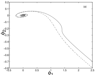
If inflation is driven by D-term, one does not get the Hubble induced mass correction to the flat direction so that . Also the Hubble induced -term is absent. However the Hubble induced mass correction eventually dominates once D-term induced inflation comes to an end.
The baryon/lepton number density is related to the dynamics of the AD field by
| (176) |
where is corresponding baryon and/or lepton charge of the AD field.The equation of motion for the AD field is given by
| (177) |
The above two equations give rise to
| (178) | |||||
The net baryon and/or lepton number can be obtained by integrating the above equation
| (179) |
Note that introduces an extra phase which can be parameterized by . Note that the asymmetry is not governed by the Hubble induced term, the amplitude of the oscillations will be damped and so the -term, which is proportional to a large power of will become gradually negligible. The net baryon and/or lepton asymmetry is given by Dine et al. (1996b)
| (180) | |||||
where . When the inflaton decay products have completely thermalized with a reheat temperature , the baryon and/or lepton asymmetry is given by
| (181) | |||||
where we have used , and is the entropy density of the universe at the time of reheating. For , the baryon-to-entropy ratio is
| (182) |
and for
| (183) |
where we have taken the net phase to be . The asymmetry remains frozen unless there is additional entropy production afterwards.
The lepton asymmetry calculated above in Eqs. (182,183) can be transformed into baryon number asymmetry via sphalerons . AD leptogenesis has important implications in neutrino physics also, because in the MSSM, the direction is lifted by the non-renormalizable operator which also gives rise to neutrino masses Dine et al. (1996b); Asaka et al. (2000a):
| (184) |
where we have assumed the see-saw relation with diagonal entries for the neutrinos , . The final can be related to the lightest neutrino mass since the flat direction moves furthest along the eigenvector of which corresponds to the smallest eigenvalue of the neutrino mass matrix Dine et al. (1996b); Asaka et al. (2000a).
| (185) |
where denotes the lightest neutrino. Similarly the case corresponds to the flat direction Enqvist and McDonald (2000); McDonald (1997).
III.3.7 Baryogenesis below the electroweak scale
At temperatures below the electroweak scale, the sphaleron transitions are rather inactive. If the universe reheats below the electroweak scale then it is a challenge to generate the required baryon asymmetry. The leptogenesis based scenarios are hard to implement below the electroweak scale. However within SM there exists a possibility of realizing cold electroweak baryogenesis as discussed in Garcia-Bellido et al. (1999); Cornwall and Kusenko (2000); Cornwall et al. (2001); Krauss and Trodden (1999); Tranberg and Smit (2003, 2006); Tranberg et al. (2010); Enqvist et al. (2010b). SUSY further opens a door to realize baryon asymmetry at temperatures even close to the BBN via R-parity violating interactions Cline and Raby (1991); Scherrer et al. (1991); Kitano et al. (2008); Kohri et al. (2009). Here we will discuss both the scenarios.
Cold electroweak baryogenesis:
There are mechanisms to obtain cold electroweak baryogenesis where it is assumed that the SM d.o.f are not in thermal equilibrium. Moreover in a cold environment the CP-violation in SM is much larger than at the electroweak temperatures, and most of the baryon asymmetry is produced at the initial quench when the Higgs field is rolling down the potential. Baryon production essentially stops after the first few oscillations, after which the coherent Higgs field will start decaying, thereby reheating the universe. However, the hurdle is to obtain this fast quench without the presence of strong first order phase transition.
There are couple of possibilities of realizing cold initial condition and out of equilibrium condition. There could be a very low scale of inflation which might not be responsible for generating the seed perturbations, or the universe could be simply trapped in a vacuum where the SM d.o.f are not even excited. The out-of-equilibrium condition can be obtained during the coherent oscillations of the scalar fields. In order to realize this idea, we would require a scalar field coupled to the SM Higgs, . During the coherent oscillations, it is possible to have the baryon number violating sphaleron transitions Garcia-Bellido et al. (1999); Tranberg and Smit (2003); Cornwall and Kusenko (2000). This can happen since the Higgs oscillations can excite the electroweak gauge bosons from the time dependent vacuum fluctuations with a very large occupation number, similar to case of preheating. These long wavelength fluctuations of the gauge fields are responsible for overcoming the sphaleron barriers which leads to the baryon number violation. Furthermore, there could be extra sources of CP-violations during the oscillations as pointed out in Cornwall and Kusenko (2000); Cornwall et al. (2001); Tranberg et al. (2010).
R-parity violation and baryogenesis:
The current limits on some of the -parity violating interactions are poorly understood. Let us now consider a scenario where B and L are violated within MSSM, with a superpotential:
| (186) |
where , , , , etc are doublets and , are singlet quarks. In Eq.(186), the first three terms violate lepton number by one unit (), while the last term violates baryon number by one unit (). For the stability of proton we assume that . This can be accomplished if there exists any conservation of lepton number, which then forces to be zero. However, the electric dipole moment of neutron gives Barbier et al. (2005)
| (187) |
and the non-observation of oscillation gives an upper bound on to be Barbier et al. (2005)
| (188) |
While is hardly constrained and can be taken to be as large as . Let us consider that a scalar field decays to MSSM d.o.f right before BBN primarily into gauge bosons and gauginos via -parity violating couplings .
Let us assume that the gauginos are heavier than the quarks and squarks. As a result their decay to a pair of quark and squark through one loop quantum correction gives rise to a net CP violation. The magnitude of CP violation in the decay: can be estimated as Cline and Raby (1991):
| (189) |
where is the trilinear SUSY breaking term and we also assume a maximal CP violation. As a result the decay of gauginos produce more squarks (antisqarks) than antisquarks (squarks). The baryon number violating () decay, induced by of squarks (antisquarks) to quarks (antiquarks) then gives rise to a net baryon asymmetry. Note that the decay of squarks (anti-squarks) are much faster than any other processes that would erase the produced baryon asymmetry. Hence the B-asymmetry can simply be given by:
| (190) |
where is the branching ratio of the decay of to , and in the above equation is the entropy density resulted through the decay of . For and GeV. Therefore a reasonable CP violation of order could accommodate the desired baryon asymmetry of close to the temperature of MeV Cline and Raby (1991); Kohri et al. (2009).
IV Dark matter
There is a conclusive evidence that a considerable fraction of the current energy density is in the form of a non-baryonic dark matter. The dynamical motions of astronomical objects such as rotation curves for spiral galaxies Begeman et al. (1991), velocity dispersion of individual galaxies in galaxy clusters, large x-ray temperatures of clusters Flores et al. (2007), bulk flows and the peculiar motion of our own local group Dressler et al. (1987), all implies the presence of a dark matter. The mass of galaxy clusters inferred by their gravitational lensing of background images is also consistent with the large dark-to-visible mass ratios Bolton et al. (2006). Perhaps the most compelling evidence, at a statistical significance of comes from the two colliding clusters of galaxies, known as the Bullet cluster Clowe et al. (2006); Markevitch et al. (2004). It was found that the spatial offset of the center of the total mass from the center of the baryonic mass peaks cannot be explained with an alteration of gravitational force law. Furthermore, the large scale structure formation from the initial seed perturbations from inflation requires a significant non-baryonic dark matter component Abazajian et al. (2009). In terms of the critical density, g cm-3 and with Hubble constant km sec-1Mpc-1, the dark matter density inferred from WMAP and large scale structure data is Komatsu et al. (2011).
The dark matter is assumed to be a weakly interacting massive particle (WIMP), yet undiscovered. There are many well motivated particle physics candidates, e.g. Jungman et al. (1996); Taoso et al. (2008); Bertone et al. (2005); Kusenko (2009), all of which arise from beyond the SM physics. The dark matter is assumed to be stable on the scale of cosmological structure formation. By virtue of new symmetries, for example R-parity conservation in SUSY allows the lightest SUSY particle (LSP) to be absolutely stable Goldberg (1983); Ellis et al. (1984a), or in the case of extra dimensions, the Kaluza-Klein (KK) parity leaves the lightest KK particle (LKP) stable Servant and Tait (2003).
In many cases some of these symmetries which protect the dark matter particle from decaying are broken by sufficiently suppressed higher-dimensional operators, such that the dark matter might as well have a finite life time comparable to the age of the universe. In the context of SUSY grand unification, operators with mass dimension are expected to make SUSY dark matter unstable, with a time-scale
| (191) |
where GeV, and is the dark matter particle. The lower dimensional operators would yield much shorter time scale, as it would lead to dark matter decay long before the structure formation. Within SUSY one compelling candidate could be the gravitino with R-parity weakly broken in the hadronic sector, yielding the required baryon asymmetry also in the process Kohri et al. (2009).
The widely accepted lore is that after radiation-matter equality, when the universe becomes matter dominated, the density perturbations in the dark matter begin to grow, and drive the oscillations of the photon-baryonic fluid around the dark matter gravitational potential wells. Immediately after the epoch of recombination the baryons kinematically decouple from photons, which then free-stream through the universe; the baryons on the other hand slowly fall into the potential wells created by the dark matter particles, eventually becoming light emitting galaxy, see for more details Kolb and Turner (1988); Peebles (1994); Dodelson (2003). There are three broad categories of dark matter which have been central to our discussion.
IV.1 Types of dark matter
IV.1.1 Hot Dark Matter
If the dark matter particle is collisionless, then they can damp the fluctuations from higher to lower density regions above the free-streaming scale. This hot dark matter consists of particles which are relativistic at the time of structure formation and therefore lead to large damping scales Bond and Szalay (1983).
The SM neutrinos are the simplest examples of hot dark matter. In the early universe they can be decoupled from a relativistic bath at MeV, leading to a relic abundance today that depends on the sum of the flavor masses:
| (192) |
Various observational constraints combining Ly- forest, CMB, SuperNovae and Galaxy Clusters data leads to Seljak et al. (2006); Fogli et al. (2008): . Similar limits can be applied to any generic hot dark matter candidate, such as axions Hannestad et al. (2010) or to hot sterile neutrinos Dodelson et al. (2006); Kusenko (2009). The free-streaming length for neutrinos is Kolb and Turner (1988):
| (193) |
For instance, the universe dominated by the eV neutrinos would lead to suppressed structures at Mpc scale, roughly the size of supercluster. Furthermore, hot dark matter would predict a top-down hierarchy in the formation of structures, with small structures forming by fragmentation of larger ones, while observations show that larger galaxies have formed from the mergers of the initially small galaxies.
IV.1.2 Cold Dark Matter
The standard theory of structure formation requires cold dark matter (CDM), whose free-streaming length is such that only fluctuations roughly below the Earth mass scale are suppressed Hofmann et al. (2001); Green et al. (2005); Loeb and Zaldarriaga (2005); Bertschinger (2006); Green et al. (2004). The CDM candidates are heavy and non-relativistic at the time of their freeze-out from thermal plasma. The current paradigm of CDM is falsifiable whose predictive power can be used to probe the structures at various cosmological scales, such as the abundance of clusters at and the galaxy-galaxy correlation functions have proven it a successful and widely accepted cosmological model of large scale structure formation.
The N-body simulations based on CDM provide a strong hint of a universal dark matter profile, with the same shape for all masses, and initial power spectrum. The halo density can be parametrized by:
| (194) |
where and the radius vary from halo to halo. the parameters and vary slightly from one profile to other. The four most popular ones are:
Amongst all the four profiles, the scales where deviations are most pronounced (the inner few kiloparsecs) are also the most compromised by numerical uncertainties. The power-law index value, , in the inner most regions is part of the numerical uncertainties and still under debate, as all four simulations provide different numbers. The simulations hint towards a cuspy profile, as the density in the inner regions becomes large, while from the rotation curves of low surface brightness (LSB) galaxies point towards uniform dark matter density profile with constant density cores Gentile et al. (2004). In our own galaxy the situation is even more murky, as the observations of the velocity dispersion of stars near the core suggests a supermassive black hole at the center of our Galaxy, with a mass Ghez et al. (1998). Many galaxies have been found to host supermassive blackholes of . It has been argued that if supermassive blackhole exists at the galactic center, the accretion of dark matter by the blackhole would enhance the dark matter density Peebles (1994). To alleviate some of these problems, dark matter with a strong elastic scattering cross section Spergel and Steinhardt (2000); Dave et al. (2001), or large annihilation cross sections Kaplinghat et al. (2000) have been proposed.
There are further discrepancies between observations and numerical simulations. The number of satellite halos as predicted by simulations exceeds the number of observed Dwarf galaxies in a typical galaxy like Milky-Way Moore et al. (1999); Klypin et al. (1999). However recent hydrodynamical simulations with CDM, including the supernovae induced outflows suggest a fall in the dark-matter density to less than half of what it would otherwise be within the central Kpc.
IV.1.3 Warm Dark Matter
Besides hot and cold dark matter, the early universe can also provide warm dark matter (WDM) candidates whose velocity dispersion lies between that of hot and CDM. The presence of WDM reduces the power at small scales due to larger free-streaming length compared to that of a CDM Bode et al. (2001); Sommer-Larsen and Dolgov (2001).
The origin of WDM can be found within sterile states. For instance, the see-saw mechanism for the active neutrino masses from the SM singlet states Minkowski (1977); Yanagida (1979); Gell-Mann and Slansky (1980); Mohapatra and Senjanovic (1981) would naturally generate masses to the active , and sterile neutrinos () in Eq. (156), if we take . The typical mixing angles in this case are: . In order to explain the neutrino masses from atmospheric and solar neutrino data, is sufficient, however for pulsar kicks Kusenko and Segre (1996, 1999); Kusenko (2006), supernovae explosion Fryer and Kusenko (2006); Hidaka and Fuller (2006, 2007), as well as sterile neutrino as a dark matter candidate Dodelson and Widrow (1994); Shi and Fuller (1999); Dolgov and Hansen (2002); Asaka et al. (2005); Abazajian et al. (2001); Petraki and Kusenko (2008), we require at least , so in total sterile Majorana states, for a review on all these effects, see Kusenko (2009). The presence of such extra sterile neutrinos is also supported by oscillations observed at LSND Aguilar et al. (2001), and the recent results by MiniBoone Aguilar-Arevalo et al. (2010).
A sterile neutrino with a KeV mass can be an ideal WDM candidate which can be produced in the early universe by oscillation/conversion of thermal active neutrinos, with a momentum distribution significantly suppressed from a thermal spectrum Dodelson and Widrow (1994); Abazajian et al. (2001). A typical free-streaming scale is given by, see Abazajian and Koushiappas (2006)
| (195) |
where is the mass of the sterile flavor eigenstate, is the mean momentum over temperature of the neutrino distribution and ranges from (for a thermal) to (for a non-thermal) distribution. Very stringent bounds on the mass of WDM particles have been obtained by different groups. Typically, the bounds range from , see Kusenko (2009). It is quite plausible to imagine a mixed dark matter scenario, where more than one species contributed to the total dark matter abundance. If there is a fraction of sterile neutrinos or WDM, then the above bounds can even be relaxed.
IV.2 WIMP production
IV.2.1 Thermal relics
At early times it is assumed that the dark matter particle, denoted by is in chemical and kinetic equilibrium, i.e. in local thermodynamic equilibrium. The dark matter will be in equilibrium as long as reactions can keep in chemical equilibrium and the reaction rate can proceed rapidly enough as compared to the expansion rate of the universe, . When the reaction rate becomes smaller than the expansion rate, then the particle can no longer be in its equilibrium, and thereafter its abundance with respect to the entropy density becomes constant. When this occurs the dark matter particle is said to be “frozen out.”
The equilibrium abundance of relative to the entropy density depends upon the ratio of the mass of the particle to the temperature. Let us define the variable , where is the number density of with mass , and is the entropy density, where counts the number of relativistic d.o.f. The equilibrium value of , for , while constant for .
The precise value of can be computed exactly by solving the Boltzmann equation Kolb and Turner (1988):
| (196) |
where dot denotes time derivative, is the total annihilation cross section, is the velocity, bracket denotes thermally averaged quantities, and is the number density of in thermal equilibrium:
| (197) |
where is the temperature. In terms of and , and using the conservation of entropy per comoving volume ( constant), we rewrite Eq. (196) as:
| (198) |
In the case of heavy , the cross section can be expanded with respect to the velocity in powers of , , where and are expressed in . Typically for s-wave annihilation, and for p-wave annihilation. We can rewrite Eq. (198) in terms of a new variable: ,
| (199) |
where prime denotes , and
| (200) |
One can find a simple analytic solution for Eq. (199) for two extreme regimes
| (201) | |||
| (202) |
Integrating the last equation for , and using , we find
| (203) |
In terms of the present energy density, , where cm-3 is the present entropy density, the relic abundance of dark matter particle in terns of the critical energy density is given by:
| (204) |
where the freeze-out temperature is defined by solving this equation iteratively for early and late time solutions, for
| (205) |
An approximate order of magnitude estimation of the abundance can be written as:
| (206) |
For a WIMP interacting with a heavy gauge boson, would naturally yield an upper bound on . From the above Eq. (206), on dimensional grounds, for , where is the mass of the new gauge boson. For TeV, abundance of the dark matter becomes of order of unity, , for . Actually, the unitarity bound limits the dark matter mass to be below TeV Griest and Kamionkowski (1990). For a realistic scenario , the unitarity bound would yield TeV.
Note that the above non-relativistic expansion of may not hold universally. When a mass of second particle becomes nearly degenerate with the dark matter particle as in the case of coannihilation Binetruy et al. (1984); Griest and Seckel (1991), or the cross section is strongly varying function of the center of mass energy as in the case of a resonant annihilation Griest and Seckel (1991). In the latter case, , gets a boost by resonant annihilation when , where annihilates with an exchange of particle, , with a mass .
IV.2.2 Coannihilating WIMPs
If there are particles, () with the lightest one, , which have nearly degenerated masses , such that , and internal d.o.f (statistical weights) . The next to lightest dark matter particle will be . In this case the above calculation of relic density, Eq. (196), gets modified Binetruy et al. (1984); Griest and Seckel (1991); Servant and Tait (2003).
| (207) |
where is the number density of the relic particle, since all other particles decay much before the long-lived . The total annihilation rate for into a SM particle is given by:
| (208) | |||||
| (209) |
is the relative particle velocity, with and are the four-momentum and energy of particle . One requires to define a thermal averaged , which is defined by:
| (210) |
where are distribution functions in the Maxwell-Boltzmann approximation.
Typically, when the scattering rate of particles off SM particles in a thermal background is much faster than their annihilation rate, then in the above Eq. (196), is replaced by:
| (211) |
where , and . In the case of co-annihilation, the freeze-out temperature is determined by
| (212) |
where and are the coefficients of the Taylor expansion of . The relic abundance for is now given by
| (213) | |||||
In any realistic framework there are many particles which interact with the dark matter candidate . They all eventually decay into , and at the time of freeze-out the density of all heavy particles is exponentially suppressed except when there is mass degeneracy occurs between heavy particles and the . The details of coannihilation has been studied extensively within SUSY Edsjo and Gondolo (1997), and publicly available numerical codes include coannihilations with all SUSY particles Gondolo et al. (2004).
IV.2.3 Non-thermal relics
The dark matter particle, , can also be created in an out of equilibrium condition, i.e. must not have been equilibrium when it froze out. A sufficient condition for non-equilibrium is that the annihilation rate (per particle) must be smaller than the expansion rate of the universe: .
Let us assume that were non-relativistic at the time of production and they were never in local thermodynamical equilibrium. The largest dark matter density will thus be determined by the largest freeze out temperature, which can be attainable in the universe. Assuming this to be the reheat temperature, and the universe follows a radiation domination, then the ratios of energy densities will be given by Kolb et al. (1998):
| (214) |
where is the present temperature and corresponds to the present time, is the energy density in radiation, and denotes the energy density in the dark matter with the number density . If we further assume that particles were created at time , sometime during the coherent oscillations of the inflaton and before the completion of reheating, then both the particle energy density and the inflaton energy density would redshift approximately at the same rate until reheating is completed. Therefore,
| (215) |
assuming that the inflaton energy density dominated the universe. Since, , where and km sec-1 Mpc-1, then using Eq. (214), one obtains Kolb et al. (1998):
| (216) | |||||
| (217) |
where is the fraction of critical energy density in radiation today, and GeV. The above expression tells us that a non-thermal creation would require a very small fraction of the inflaton energy density to be transferred to the dark matter particle , otherwise the universe would be dominated by the dark matter particles.
For a singlet hidden sector dark matter, it is really a challenge not to overproduce them directly from the decay of the inflaton. If the inflaton sector belongs to the hidden sector, then it is natural to have inflaton couplings to such hidden sector dark matter field. There are three possible ways to obtain a small fraction of in order to match the current observations.
(a) Gravitational production
The dark matter can be created from the transition of the equation of state of the universe from inflation to matter domination or radiation domination, due to non-adiabatic evolution of the vacuum Kolb et al. (1998); Chung et al. (1999b); Chung et al. (2001, 2000). The underlying mechanism is similar to the metric fluctuations which seed the structure formation, except now the excitations can create massive particles. The gravitational production of dark matter is universal, and it can occur even if the dark matter coupling to the inflaton is vanishingly small.
Let us consider a simple action for field with a metric , where is a conformal time.
| (218) |
where is the Ricci scalar. Let us expand the field in terms of creation and annihilation operators which obey: , and
| (219) |
where the mode functions obey the identity , and prime denotes derivative w.r.t. . The mode equation is given by:
| (220) |
The parameter for conformal and for minimal coupling. Here we will consider the conformal coupling for simplicity. The number density of particles can be estimated by a Bogoliubov transformation:
| (221) |
where , and . The energy density of produced particles is given by Chung et al. (1999b):
| (222) |
where the number operator is defined at . Assuming that the transition from inflation-radiation or matter domination is smooth, the largest energy density can be obtained if . If . If GeV and is the mass of the inflaton, then particles produced gravitationally can match the density today of the order of the critical density provided they are long lived. Such super heavy massive dark matter particle is known as Wimpzillas!
(b) Direct decay of the inflaton
The dark matter can also be created from direct inflaton decay if , with a rate , where is the interaction strength. The total inflaton decay rate is given by , while the inflaton number density at the time of decay is given by . This constrains the overall coupling to
| (223) |
where is in units of GeV. This is required due to the fact that the produced must not overclose the universe which, for and km , reads
| (224) |
when is expressed in units of GeV Allahverdi et al. (2002). It is evident from the overclosure bound that needs to be very small.
(c) Creation during reheating
If the process of reheating is slow and not instantaneous, then it is possible to create WIMP from the ambient plasma which is in the process of acquiring thermalization via scatterings. The Boltzmann equations for inflaton energy density, , radiation energy density, , and dark matter energy density are given by Kolb and Turner (1988); Chung et al. (1999a):
| (225) |
where dot denotes time derivative, and thermal averaged cross section is given by: . The equilibrium energy density for the particles, , is determined by the radiation temperature, . Following Chung et al. (1999a); Kolb and Turner (1988), it is useful to introduce two dimensionless constants, and , defined in terms of , , and . With these parameters the Boltzmann equations are:
| (226) |
where , prime denotes , and the constants , , and are given by
The equilibrium value of is given in terms of the temperature and Eq. (197): .
It is straightforward to solve the system of equations in Eq. (IV.2) with initial conditions at , , and . At early time solution for can be easily obtained:
| (227) |
By maximizing the above equation, which is obtained at , the largest temperature of the ambient plasma can be even larger than the reheat temperature Kolb and Turner (1988)
| (228) |
From Eq. (227) when , scales as , which implies that entropy is created in the early-time regime. For the choices of , , , and , and Chung et al. (1999a):
| (229) |
(d) Non-perturbative creation of dark matter
The dark matter can be created non-perturbatively during the coherent oscillations of the inflaton.
Superheavy dark matter during preheating:
If the dark matter couples to the inflaton directly, then it is more efficient to excite them from the coherent oscillations of the inflaton during preheating. One of the most interesting applications of preheating is the copious production of particles which have a mass greater than the inflaton mass . Such processes are impossible in perturbation theory and in the theory of narrow parametric resonance.
Following Eq. (101), let us suppose that the dark matter is coupled to the inflaton with an interaction term: . During the broad resonance regime, as we have discussed in section II.6.1, superheavy -particles with mass can be produced. The momentum dependent frequency violates the adiabatic condition of time dependent vacuum, see Eq. (107), when
| (230) |
where is the amplitude of the inflaton oscillations. The maximal range of momenta for which particle production occurs corresponds to , where . The maximal value of momentum for particles produced at that epoch can be estimated by . The resonance becomes efficient for . Thus, the inflaton oscillations may lead to a copious production of superheavy particles with if the amplitude of the field is large enough, Kofman et al. (1997).
Dark matter from the fragmentation of a scalar condensate:
Let us assume that coherent oscillations of a scalar condensate in a potential has a frequency which is large compared to the expansion rate of the universe. The equation of state is obtained by averaging, , over one oscillation cycle . The result is: , where Turner (1983). For the case , one finds , so that one effectively obtains the usual case of pressureless, non-relativistic cold matter. When the motion of the condensate is not simply oscillatory, such as in the case of a rotating trajectory with a phase, one can generalize the above calculation by integrating over the orbit of the condensate. Let us consider the potential
| (231) |
one finds that . There arises a negative pressure whenever . This is a sign of an instability of the scalar field under arbitrarily small perturbations. The quantum fluctuations in the condensate grow according to when effective mass of the scalar field is much larger than the expansion
| (232) |
If , quantum fluctuations of the condensate at the scale, , will grow exponentially in time:
| (233) |
In reality the onset of non-linearity sets the scale at which the spatial coherence of the field can no longer be maintained and the condensate fragments. The initial fluctuations in the condensate owes to the inflationary perturbations. If the condensate carries a global charge, due to charge conservation the energy-to-charge ratio changes as the the condensate fragments. This is what happens in the case of MSSM. The AD condensate which was responsible for generating the baryon asymmetry at the first instance could fragment Kasuya and Kawasaki (2000b, a); Kusenko et al. (2009). The ground state of these fragmented lumps is a non-topological soliton with a fixed charge, called the -ball Coleman (1985); Lee and Pang (1992); Kusenko (1997b). In gauge mediated SUSY breaking scenarios the -balls can absolutely stable and can be a candidate for CDM Kusenko et al. (1998); Kusenko and Shaposhnikov (1998); Kusenko and Shoemaker (2009). The -balls can also be formed from the fragmentation of the inflaton Enqvist et al. (2002a, b). The slow surface evaporation of a -ball will also create SUSY LSP, which we will discuss below.
IV.3 Candidates
In this subsection we will discuss some of the dark matter candidates which are well motivated, and the challenges they face.
IV.3.1 Primordial blackholes
The primordial blackholes (PBH) can be created in the early universe Hawking (1971); Carr and Hawking (1974), and they can survive the age of the universe with a typical lifetime of an evaporating blackhole which is given by:
| (234) |
If the initial mass g, the blackhole will be evaporating now, for heavier blackholes the Hawking evaporation is negligible, and they can be a CDM candidate. When g, the blackholes would decay at the time of BBN. The PBHs are formed from the collapse of order one perturbations, , inside the Hubble patch. The detailed numerical simulation suggest Niemeyer and Jedamzik (1998, 1999); Jedamzik and Niemeyer (1999). In a radiation dominated epoch the blackhole mass is bounded by the Hubble mass
| (235) |
where is temperature of the thermal bath during radiation. In spite of novelty in this idea, the detailed calculations suggest that it is hard to form primordial blackholes just from the collapse of sub-Hubble over densed regions - one requires more power on small scales in Carr and Lidsey (1993); Green and Liddle (1997); Drees and Erfani (2011), while the CMB data points towards . It was shown in a hydrodynamical simulation Jedamzik and Niemeyer (1999) that primordial blackholes can also be produced in a first order phase transition, and during preheating Green and Malik (2001).
The abundance of PBH contains many uncertainties, as the details of the initial gravitational collapse and the initial number density of depends on many physical circumstances. These uncertainties can however be encoded in terms of the ratio determined by the initial time, ; , by assuming ,
| (236) |
where corresponds to present time. In terms of this fraction , the PBH abundance is given by Carr (1975); Green and Liddle (1999)
| (237) |
The value of can be constrained from , which yields , for mass g. A tighter constrain on arises from a range of astrophysical observations, such as BBN, CMB anisotropy, and -ray backgrounds for g, the bound weakens for larger mass blackholes Carr et al. (2010).
IV.3.2 Axions
The axions were introduced to solve the strong CP problem Peccei and Quinn (1977b, a) which requires a new global chiral symmetry that is broken spontaneously at the Peccei-Quinn (PQ) scale (for reviews, see Kim (1987); Turner (1990); Raffelt (1990); Sikivie (2008)). The corresponding pseudo-Nambu-Goldstone boson is the axion Weinberg (1978); Wilczek (1978), which couples to the gluons
| (238) |
where is the color anomaly of the PQ symmetry depends on the interactions. This interaction term compensates the vacuum contribution in the QCD Lagrangian , in a way that Nakamura et al. (2010), in order to match the electric dipole moment of the neutron. The dynamical solution yields when , at which the effective potential for the axion has its minimum.
The axion can interact via heavy quark while all other SM fields do not carry any PQ charge, in which case Kim (1979); Shifman et al. (1980). The axion can directly couple to the SM, and at the lowest order it will induce non-renormalizable coupling with the gluons, where Dine et al. (1981); Zhitnitsky (1980).
The axion searches, various astrophysical and cosmological observations suggest that the PQ scale Sikivie (2000); Raffelt (2008); Nakamura et al. (2010) must be large,
| (239) |
and the axion mass must be very small, eV. The cosmological constraints on GeV ( eV) arises from BBN, accounting for the current bound on the relativistic species, Iocco et al. (2009). Another interesting bound arises from isocurvature perturbations from CMB. At best one can allow less than of the total perturbations to arise from sources other than the inflaton fluctuations–the axions being massless during inflation can account for such fluctuations, which limits GeV, however, it depends on the scale of inflation Beltran et al. (2007); Steffen (2009).
The axion life time depends on the axion-photon interaction, which gives a long life time compared to the age of the universe, i.e., s for Kolb and Turner (1988).
Axion is massless for and it acquires mass only through instanton effects for . For GeV (corresponding to eV), the axion is a thermal relic that decouples after the quark–hadron transition, MeV. The axion is kept in thermal equilibrium with . The relic thermal abundance is given by , where denotes the number of effectively massless degrees of freedom.
In an opposite limit, when is very large, the axions are never in thermal equilibrium, and in particular when the PQ symmetry is never restored. The main production mechanism is due to the coherent oscillations of the axion due to the initial misalignment angle of the axion. At , the axion obtains a temperature dependent effective mass and oscillate coherently around its minimum when . These oscillations of the axion condensate behaves as cold dark matter Preskill et al. (1983); Abbott and Sikivie (1983); Dine and Fischler (1983) with a relic density that is governed by the initial misalignment angle Beltran et al. (2007); Sikivie (2008):
| (240) |
with parametrizing theoretical uncertainties related to details of the quark–hadron transition and accounting for anharmonicity in – for . For GeV, this “misalignment mechanism” can provide the correct dark matter abundance.
IV.4 SUSY WIMP
The most general gauge invariant and renormalizable superpotential would also include baryon number or lepton number violating terms, with each violating by one unit: and , where represents the family indices. The chiral supermultiplets carry baryon number assignments for , for , and for all others. The total lepton number assignments are for , for , and for all the others. Unless and terms are very much suppressed, one would obtain rapid proton decay which violates both and by one unit.
There exists a discrete symmetry, which can forbid baryon and lepton number violating terms, known as -parity Fayet (1979). For each particle:
| (241) |
with for the SM particles and the Higgs bosons, while for all the sleptons, squarks, gauginos, and Higgsinos. Here is spin of the particle. Besides forbidding and violation from the renormalizable interactions, -parity has interesting phenomenological and cosmological consequences. The lightest sparticle with , the LSP, must be absolutely stable. If electrically neutral, the LSP is a natural candidate for dark matter Ellis et al. (1984a); Dimopoulos and Hall (1988). The advantage here is that their cross sections are governed by the SM gauge group – and therefore the dark matter paradigm is embedded within a visible sector. However, there are some exceptions which we will discuss first.
IV.4.1 Gravitino
The gravitino is a spin- supersymmetric partner of the graviton, which is coupled to all the sectors universally, e.g. visible and hidden sectors, with a Planck suppressed interaction. In this respect gravitino is truly a singlet dark matter candidate, if it happens to be the LSP. The gravitino mass can vary ( KeV) depending on the details of the SUSY breaking schemes, for instance, in gauge and gravity-mediated SUSY breaking scenarios Dine et al. (1995a, 1996a); Giudice and Rattazzi (1999). Indeed, without considering the SUSY breaking mechanisms and the SUSY breaking scale, we can treat the gravitino mass as a free parameter.
Production: Gravitinos with both the helicities can be produced from a thermal bath, they are never in thermal equilibrium. They are produced mainly through the scatterings–within MSSM there are many scattering channels which include fermion, sfermion, gauge and gaugino quanta all of which have a cross-section . The thermal abundance is given by (up to a logarithmic correction) for as in the case of MSSM: Ellis et al. (1984b), and Bolz et al. (2001), where is the gluino mass.
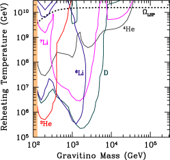
Note that for both the helicity states have essentially the same abundance, while for production of helicity states is enhanced due to their Goldstino nature. The net abundance can be approximated by the convenient expression for the universal gaugino masses at and Pradler and Steffen (2008)
| (242) |
Thermally produced gravitinos have a negligible free-streaming velocity today. However, the gravitinos created from decays can be warm or hot dark matter.
Besides thermal production, gravitino can be produced non-thermally from the decay of the NLSP (next-to-lightest SUSY particle). Obviously different NLSP’s give slightly different abundances. For sneutrino, see Refs. Feng et al. (2004); Arina and Fornengo (2007); Ellis et al. (2008), for stop NLSP, see Kang et al. (2008); Diaz-Cruz et al. (2007); Berger et al. (2008). A simple approximation yields Steffen (2006); Pospelov et al. (2008)
| (243) |
where the total slepton number density is given by assuming an equal number density of positively and negatively charged slepton’s. The NLSP’s can have a long lifetime . For a slepton NLSP, one finds in the limit ,
| (244) |
which holds not only for a charged slepton NLSP but also for the sneutrino NLSP. Similar expressions for the lifetimes for the neutralino NLSP Feng et al. (2004) and the stop NLSP can be found inDiaz-Cruz et al. (2007). If the NLSP decays into the gravitino LSP after BBN, the SM particles emitted in addition to the gravitino can affect the abundances of the primordial light elements. Also the presence of a long-lived negatively charged particle, champ, i.e. , can lead to bound states that catalyze BBN reactions Dimopoulos et al. (1990); De Rujula et al. (1990). The new acceptable limits on champs: TeV, virtually ruled out any low scale SUSY champs Chuzhoy and Kolb (2009). It was suggested in Ref. Pospelov (2007) that bound-state formation of champ with can lead to a substantial production of primordial , which puts the constraint sec. Pospelov (2007); Hamaguchi et al. (2007); Bird et al. (2008); Takayama (2008); Pradler and Steffen (2008); Pospelov et al. (2008).
Uncertainties: The main uncertainties on gravitino abundance arise from the hidden sectors. If the inflaton sector is embedded within a hidden sector then there are many more sources of gravitino production–the inflaton could decay directly into gravitino during reheating or preheating Maroto and Mazumdar (2000); Giudice et al. (1999b); Nilles et al. (2001a); Kallosh et al. (2000a, b); Nilles and Peloso (2001); Frey et al. (2006), the inflaton couplings to other hidden sectors can similarly excite gravitinos giving rise to large uncertainties in their total abundance.
| (245) |
All these contributions can easily overproduce gravitinos, i.e. , especially the last two sectors are largely unconstrained by particle physics. These uncertainties can be minimized if the last phase of inflation occurs within MSSM, as discussed in Sect. LABEL:GGIOM, then the only predominant source of gravitino production arises from the decay of the MSSM inflaton and from the MSSM thermal bath.
Another solution has been put forward – for high scale and hidden sector models of inflation – since the flat directions of MSSM can be displaced from their minimum during inflation, the flat direction VEV at early times would generate time dependent masses to the MSSM fields which are coupled to the flat direction. As a result, the inflaton might not even decay into all the MSSM d.o.f due to kinematical blocking Allahverdi and Mazumdar (2005); Allahverdi and Mazumdar (2006b, 2007b). Furthermore, the flat direction VEV also generates masses to gauge bosons and gauginos which participate in scatterings, therefore delaying the actual thermalization process and lowering the reheating temperature, i.e. . Both these effects address the thermal gravitino overproduction problem without any need of extra assumptions Allahverdi and Mazumdar (2005).
Unstable gravitino: An unstable gravitino decays to particle-sparticle pairs, and its decay rate is given by . If TeV, the gravitinos decay during or after BBN, which can ruin its successful predictions for the primordial abundance of light elements Cyburt et al. (2003); Kawasaki et al. (2005). If the gravitinos decay radiatively, the most stringent bound, , arises for TeV Cyburt et al. (2003). On the other hand, much stronger bounds are derived if the gravitinos mainly decay through the hadronic modes. In particular, for a hadronic branching ratio , and in the same mass range, will be required Kawasaki et al. (2005, 2008). This puts constraint on reheat temperature of the universe, i.e. , at which these unstable gravitinos are produced, see Fig. 5. An intriguing possibility arises if R-parity is broken. The gravitino LSP with GeV can still be a long-lived cold dark matter, while evading the bounds on from Fig. 5. The gravitino in this case cannot decay into hadrons which is kinematically suppressed, and the three-body decay life time is typically larger than the age of the universe Kohri et al. (2009). For a GeV mass gravitino, the present day free-streaming velocity is km/s, which corresponds to that of a cold dark matter.
Detection: The direct detection of gravitino will be impossible at the LHC, their production will be extremely suppressed. If the NLSP is long lived (quasi-stable) as in the case of stau then they would penetrate the collider detector in a way similar to muons Drees and Tata (1990); Nisati et al. (1997); Feng and Moroi (1998). If the produced staus are slow, then from the associated highly ionizing tracks and time of flight measurements one can determine their mass Ellis et al. (2006). This might give some indirect handle on gravitinos.
IV.4.2 Axino
The axino, , is a superpartner of the axion, is another example of a gauge singlet dark matter candidate Nilles and Raby (1982); Kim and Nilles (1984); Kim (1984). It interacts extremely weakly since its couplings are suppressed by the PQ scale GeV Sikivie (2008); Raffelt (2007, 2008), and its mass can range from eV to GeV. In the hadronic axion model Kim (1979); Shifman et al. (1980) in a SUSY setting, the axino couples to MSSM field indirectly via loops of heavy (s)quarks. Typically decouples early at a temperature GeV, below this temperature, they are mainly created from scatterings of MSSM fields in an kinetic equilibrium. The thermal abundance is given by Brandenburg and Steffen (2004); Covi et al. (2001); Choi et al. (2008)
| (246) | |||||
with the axion-model-dependent color anomaly of the PQ symmetry breaking scale . Thermally produced axinos can be hot, warm, and cold dark matter Covi et al. (2001) as shown in Fig. 6.
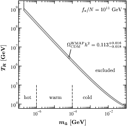
Non-thermal production of has many uncertainties. The can be created from the decay of the NLSP, direct decay from the inflaton or moduli, or any other hidden sector. The expression for the final abundance is similar to that of Eq. (245), where . In this regard faces similar challenges as that of a gravitino dark matter.
The LSP is inaccessible in direct/indirect dark matter searches if R-parity is conserved. Their direct production at collider is strongly suppressed. Nevertheless, quasi-stable ’s could appear in collider detectors (and neutrino telescopes Albuquerque et al. (2007); Ahlers et al. (2006)) as a possible signature of the LSP.
IV.4.3 Neutralino
In the MSSM the binos (superpartner of B), winos (superpartner of ) and Higgsinos ( and ) mix into Majorana fermion eigenstates, called neutralinos with mass eigenstates: , ordered with increasing mass. The LSP is thus denoted by . The gaugino fraction, , and Higgsino fraction, , are determined by the mixing matrix, , which diagonalizes the neutralino mass matrix Kane et al. (1994); Jungman et al. (1996).

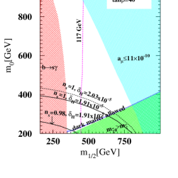
The ’s were in thermal equilibrium for primordial temperatures of . At , the annihilation rate of the (by then) non-relativistic ’s becomes smaller than the Hubble rate so that they decouple from the thermal plasma, see Sect. IV.2.1.
It is easy to work with a limited set of parameters, the mSUGRA model is a simple model which contains only five parameters:
| (247) |
is the universal scalar soft breaking parameter, is the universal gaugino mass, is the universal cubic soft breaking mass, measures at , and at the electroweak scale.
The model parameters are already constrained by different experimental results. (i) the light Higgs mass bound of GeV from LEP Barate et al. (2003), (ii) the branching ratio bound of (we assume here a relatively broad range, since there are theoretical errors in extracting the branching ratio from the data) Alam et al. (1995), (iii) the 2 bound on the dark matter relic density: Komatsu et al. (2009), (iv) the bound on the lightest chargino mass of 104 GeV from LEP Nakamura et al. (2010) and (v) the muon magnetic moment anomaly , where one gets a 3.3 deviation from the SM from the experimental result Bennett et al. (2004).
The allowed mSUGRA parameter space, at present, has mostly three distinct regions: (i) the stau-neutralino (), coannihilation region where is the lightest SUSY particle (LSP), (ii) the having a dominant Higgsino component (focus point) and (iii) the scalar Higgs (, ) annihilation funnel (2). These three regions have been selected out by the CDM constraint. There stills exists a bulk region where none of these above properties is observed, but this region is now very small due to the existence of other experimental bounds. The allowed parameter space for the neutralino dark matter (blue region) for is shown in the left panel of Fig. 7.
Detection: In general the observable signals for SUSY at LHC are: leptons+ jets + (missing transverse energy), where either or could be . The existence of missing energy in the signal will tell us the possibility of dark matter candidate. There are SM backgrounds, e.g. and bosons decaying to neutrinos providing . The clean signal for SUSY would be jets + , without isolated leptons. One of the key analysis for mSUGRA is to measure the which is the sum of the transverse momenta of the four leading jets and the missing transverse energy: . One has to further measure the masses (squarks, sleptons), and , and the mixing matrices which lead to the calculation of the relic density. One particularly favored parameter space is the coannihilation region where the stau and the neutralino masses are close for smaller values of . The mass difference, , governs the relic abundance due to the Boltzmann suppression factor , see section IV.2.2. Therefore measuring directly gives handle on measuring the relic abundance at the LHC, see for a detailed discussion in Nath et al. (2010).
MSSM inflation and dark matter: After considering all these bounds it was found that there exists an interesting overlap between the constraints from MSSM inflation and the abundance, see the right hand panel of Fig. 7 for . The constraints on the parameter space arising from the inflation appearing to be consistent with the constraints arising from the dark matter content of the universe and other experimental results.
It is also interesting to note that the allowed region for as an MSSM inflaton with a mass , required by the CMB observations for , see Fig. 3 in Sect. II.5.2, lies in the stau-neutralino coannihilation region which requires smaller values of the SUSY particle masses Allahverdi et al. (2007a). Similar analysis were performed in Balazs et al. (2005, 2004), where the authors studied the overlap between MSSM parameters for the electroweak baryogenesis and the dark matter abundance.
IV.4.4 Sneutrino
The lightest right handed (RH) sneutrino can be a good dark matter candidate when the SM gauge group is augmented to , with a superpotential Allahverdi et al. (2007b, 2010b)
| (248) |
The model introduces new gauge boson , two Higgs fields , and their superpartners, the Yukawa coupling is denoted by . The spontaneous breaking of will generate Majorana neutrino masses, or if , then Dirac neutrino masses, or a mixture of both Dirac and Majorana Allahverdi et al. (2011a). If the right handed sneutrino is the LSP then it provides another compelling candidate which is well motivated from particle theory and can be embedded with least unknown uncertainties Allahverdi et al. (2007b); Arina and Fornengo (2007); Lee et al. (2007).
Scatterings via the new gauge interactions bring the RH sneutrino into thermal equilibrium. In order to calculate the relic abundance of the RH sneutrino, we need to know the masses of the additional gauge boson and its SUSY partner , the new Higgsino masses, Higgs VEVs which break the new gauge symmetry, the RH sneutrino mass, the new gauge coupling, and the charge assignments for the additional . The primary diagrams responsible to provide the right amount of relic density are mediated by in the -channel
By assuming that the new gauge symmetry is broken around TeV in Fig. 8, we show the relic density values for smaller masses of sneutrino where the lighter stop mass is TeV. The smaller stop mass will be easily accessible at the LHC. By varying new gaugino and Higgsino masses and the ratio of the VEVs of new Higgs fields, the WMAP Komatsu et al. (2009) allowed values of the relic density, i.e., is satisfied for many points. In the case of a larger sneutrino mass in this model, the correct dark matter abundance can be obtained by annihilation via pole Lee et al. (2007); Allahverdi et al. (2007b).

Detection: Since the dark matter candidate, the RH sneutrino, interacts with quarks via the boson, it is possible to see it via the direct detection experiments. The detection cross sections are not small as the interaction diagram involves in the -channel. The typical cross section is about 2 pb for a mass around 2 TeV. It is possible to probe this model in the upcoming dark matter detection experiments. The signal for this scenario at the LHC will contain standard jets plus missing energy and jets plus leptons plus missing energy. The jets and the leptons will be produced from the cascade decays of squarks and gluinos into the final state containing the sneutrino.
IV.4.5 Stable and evaporating Q-ball, LSP dark matter
The AD condensate fragments to form Q-balls, for reviews see Enqvist and Mazumdar (2003); Dine and Kusenko (2004), and a finite size Q-ball has a minimum of energy and it is stable with respect to decay into free quanta if min, for .
For a sufficiently large , the energy of a soliton is then given by Coleman (1985); Kusenko (1997b); Lee and Pang (1992): , which ensures its stability against decay into plane wave solutions with inside and outside the soliton, where . The value of was computed in Kusenko (1997a, b). Note that the global symmetry is thus broken inside the soliton by the VEV, however, remains unbroken outside the soliton. The most crucial piece is the presence of a global charge of the -ball which actually prevents it from decaying and makes the soliton stable.
In the context of gauge mediated SUSY breaking the AD potential takes the form Kusenko and Shaposhnikov (1998); Dvali et al. (1998), where , represents the SUSY breaking scale. The profile of the -ball is given by , where the energy, radius and the VEV of a -ball goes as Kusenko and Shaposhnikov (1998); Enqvist and Mazumdar (2003)
| (249) |
This allows for the existence of some entirely stable Q-balls with a large baryon number (B-balls). Indeed, if the mass of a B-ball is , then the energy per baryon number is less than 1 GeV for . Such large B-balls cannot dissociate into protons and neutrons and are entirely stable – thanks to the conservation of energy and the baryon number. If they were produced in the early universe, they would exist at present as a form of dark matter Kusenko and Shaposhnikov (1998). There are astrophysical and terrestrial lilmits Kusenko et al. (1998); Kusenko and Shoemaker (2009), and direct searches for the Q-balls, which places a lower limit on Arafune et al. (2000).
In the gravity mediated case the -balls are not stable, but they evaporate via surface evaporation. In this process AD condensate can generate the required baryon asymmetry and also create dark mater. The appropriate candidate will be the flat direction, lifted by operator, which carries the baryon number and the right dark matter abundance, see Eq. (183).
When a -ball decays, for each unit of produced, corresponding to the decay of squarks to quarks, there will be at least three units of -parity produced, corresponding to at least LSPs (depending on the nature of the cascade produced by the squark decay and the LSP mass, more LSP pairs could be produced). Let be the number of LSPs produced per baryon number and be the fraction of the total asymmetry contained in -balls. Then the baryon to dark matter ratio, , and the dark matter abundance are given by Enqvist and McDonald (1998, 1999),
| (250) |
where is the nucleon mass and is the LSP mass. It is rather natural to have .
The LSPs produced in -ball decays will collide with themselves and with other weakly interacting particles in the background and settle locally into a kinetic equilibrium. Thermal contact can be maintained until , and a rough freeze-out condition for LSPs (if they were initially in thermal equilibrium) will be given by: , where is the LSP annihilation cross-section and the subscript refers to the freeze-out values. The thermally averaged cross section can be written as , where and depend on the couplings and the masses of the light fermions Jungman et al. (1996).
Assuming an efficient LSP production, so that , one finds for the LSP density for , where . The LSPs produced in -ball decays will spread out by a random walk with a rate determined by the collision frequency divided by a thermal velocity . Since the decay is spherically symmetric, it is very likely that the LSPs have a Gaussian distribution. In terms of the density parameter , the neutralino abundance can be written as Fujii and Hamaguchi (2002)
| (251) |
where the decay temperature of the B-ball is given by
| (252) |
Below this temperature the annihilations of are negligible. Similar analysis can be performed for other LSP candidates. For example, if the gravitino is an LSP, the gravitino abundance from the Q-balls decay will be given by Shoemaker and Kusenko (2009):
| (253) |
where and . The above expression is valid for temperatures below GeV. Similar expression can be derived for the Q-balls decaying into axino dark matter Roszkowski and Seto (2007).
IV.5 Detection of WIMP
The direct detection of WIMP is the cleanest way to seek the identity of the dark matter, their detection is possible through elastic collision with the nuclei at terrestrial targets Goodman and Witten (1985). This method is especially promising for detecting SUSY WIMP candidates, such as neutralino or sneutrino. There are also ways of inferring WIMP in the sky by using the galaxy itself as a detector in the indirect dark matter searches via studying the gamma rays, high energy neutrinos, charged leptons, proton, anti-proton background from the decay or annihilation of the dark matter particles.
IV.5.1 Direct detection of WIMPs
Important quantity is the recoil energy deposited by the WIMP interaction with the nucleus of mass in an elastic collision, , where is the WIMP nucleus reduced mass, is the scattering angle in the dark matter-nucleus center-of-mass frame, and is the velocity relative to the detector, and it is of the order of the galactic rotation velocity km/s. Typical recoil energies are keV.
The differential rate for WIMP elastic scattering off nuclei is given by Lewin and Smith (1996)
| (254) |
where represents the number of the target nuclei, is the dark matter mass and is the local WIMP density in the galactic halo, and are the WIMP velocity and velocity distribution function in the Earth frame, which we take it to be Maxwellian, and is the WIMP-nucleus differential cross section. The velocity , and is the escape velocity of the WIMP in the Earth frame, km/s.
In fact, the Earth velocity with respect to the dark matter halo must be written as where is the galactic velocity of the Sun and year. The modulation is due to the rotation of the Earth around the Sun Drukier et al. (1986); Freese et al. (1988). In the above expression, must be replaced by . There also exists a forward-backward asymmetry in a directional signal as first pointed out in Spergel (1988); Copi et al. (1999).
For a given momentum transfer , the differential cross section depends on the nuclear form factor
| (255) |
where is a dimensionless form factor such that , in which case corresponds to the total cross-section. It is possible to estimate the parameters and , for example in the case of neutralino WIMP, which is a Majorana fermion therefore it only has axial and scalar couplings Jungman et al. (1996).
Spin-dependent cross-section:
The axial part of the neutralino-quark interaction is mediated via Z boson and squark exchange . At the level of nutralino-nucleon interaction by considering the nucleon matrix element , the effective Lagrangian is given by: , where is the Fermi constant and is a dimensionless parameter. For a nucleus of spin J, with and being the average spins “carried” by protons and neutrons respectively, the cross-section at zero momentum transfer is given by Jungman et al. (1996)
| (256) |
where . Additional corrections to the form factor is required to take into account of the non-zero momentum transfer. There are many experiments which are sensitive to spin-dependent cross section with pure proton couplings, DAMA Bernabei et al. (2004), PICASSO Archambault et al. (2009), KIMS Lee et al. (2007). Recently COUPP Behnke et al. (2011) has set the best constraint on spin-dependent cross section down to for a WIMP mass GeV.
Spin-independent cross-section:
The scalar part of the neutralino-quark interaction is mediated via Higgses and squark exchanges: . To express the neutralino-nucleon coupling one needs the nucleon matrix element , the effective interaction has the form: , where contains the information about hadron physics, and typically it is the same for proton or neutron, i.e., . In the case of right handed sneutrino also there exists no spin-dependent part as it has no axial-vector interactions, and the cross-section is dominated by the spin-independent part. One can define a single spin-independent WIMP-nucleon cross section , independent of the spin of the nucleon Jungman et al. (1996).
| (257) |
In the spin-independant case, for low nuclear recoil energies , there is a coherence effect which boosts the WIMP-nucleus cross section by a factor . As a result this technique is better suited to detect the WIMP candidate with heavy nucleus targets. Recently the most stringent limits on the elastic spin-independent WIMP-nucleon cross-section has been given by number of experiments, such as CDMS-II Ahmed et al. (2010), EDELWEISS-II Armengaud et al. (2011) and XENON100 Aprile et al. (2011). These limits are shown in Fig. 9. The shaded gray area also shows the expected region of CMSSM for the WIMP mass and the cross section are indicated at and CL Buchmueller et al. (2011). The current results also covers the CL areas favored by CoGeNT (green) Aalseth et al. (2011) and DAMA (light red) Savage et al. (2009).
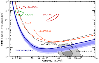
It should be noted that CoGeNT Aalseth et al. (2011), and DAMA/NaI Bernabei et al. (2004) and DAMA/LIBRA Bernabei et al. (2008) collaborations have observed an annual modulation signal. The combined results of the latter group stands at greater than statistical significance. The modulation signal phase matches well with the expected annual signal of WIMPS, and subsequent data Bernabei et al. (2010) has increased the statistical significance of the modulation signal. However the annual modulation claim has not been verified by any other experiments, especially the null results from CDMS, XENON10, and XENON100 data. The CDMS data Ahmed et al. (2010) shows signal events with events expected as background, but due to low statistics this result has not provided sufficient evidence for the dark matter.
IV.5.2 Indirect detection
The indirect dark matter detection depends on the nature of the WIMP. If the WIMP belongs to the visible sector, or if it has some SM interactions, then their annihilation or decay would yield to the known particle physics spectrum, for a recent review on indirect detection, see Porter et al. (2011). However the spectrum would depend on where they are produced, their energy deposition, and what are their final states, e.g. etc. The signal could be a hard spectrum with a monochromatic line if WIMPS annihilate directly into photons Bergstrom et al. (1998), or a continuum spectrum if they annihilate into a pair of intermediate particles (). The former process is generically suppressed compared to the latter. Most of these latter particles, i.e. decay into , , and a tiny fraction of deuterium or anti-deuterium /. The s decay to gamma rays, while the decays produce . If the final states of decay or annihilations are s or s, they dominantly produce a hard spectrum, with the decays into and . If the final states have , they produce a softer spectrum and a strong neutrino signal. The can also decay hadronically to pions and thus can also produce a strong -ray signal.
The source spectrum is generically given by
| (258) |
where denotes the annihilating final states, each with branching fraction with being the energy of secondary particles. The production rate per annihilation of species is given by . For a decaying dark matter can be replaced by , where is the decay rate.
The flux of such final states would depend on the annihilation or decay rate, which in turn would depend on the dark matter density . Therefore, the natural sources to look at in the sky are the nearby galactic centers – where there are large astrophysical uncertainties, dwarf galaxies – which have small astrophysical background, and galactic centers – where the dark matter density is very large but distant sources would yield a local tiny flux.
Gamma rays and neutrinos are perhaps the cleanest signals if they are produced as a result of WIMP annihilations or decays as they are undeflected by magnetic fields and effectively indicating the direction to their source. The flux is given by the integral of the WIMP density-squared along the line of sight from the observer to the source, multiplied by the production spectrum
| (259) |
where denotes the final states and the coordinate runs along the line of sight, is the gamma-ray energy, and is the elongation angle with respect to the center of the source. The astrophysics related term is hidden in Bergstrom et al. (1998)
| (260) |
where the integration is in the direction along the line . The above expression is also valid for neutrinos if the source is not far away from us.
On the other hand the charged particles do not have the directional sensitivity, they lose it in their course of path in a random motion due to the interstellar magnetic field. The motion of are deflected by the interstellar radiation field by synchroton radiation in presence of magnetic field. If produced at energies GeV and if their sources are within few kiloparsecs, then they can reach the solar system. Furthermore, the cosmic rays from the primary and secondary products can also generate rays during their course through the ISM, all these effects can be captured numerically in the publically available code GALPROP Strong and Moskalenko (1998); Strong et al. (2000, 2004), for a review see Strong et al. (2007).
The main challenge is to disentangle the WIMP signals from astrophysical backgrounds, the powerful discriminator is the spectral tilt in the power spectrum. It is quite possible to have a significant fraction of WIMP annihilation or decay into monoenergetic photons, giving rise a distinctive line in the gamma-ray spectrum Bergstrom et al. (1998), but the likely signal would be to have a relatively hard continuum spectrum with a bump or edge near the WIMP mass that is above the astrophysical background.
In recent years there have been many new experiments which have propelled the indirect search for dark matter research vigorously. For instance, the ATIC data – which shows a significant bump in the electron flux around GeV Chang et al. (2008), where conventional astrophysical sources would have predicted a decaying power law spectrum, and the PAMELA – which shows a positron fraction which has a rising slope above GeV Adriani et al. (2009, 2010), but the anti-proton flux and the fraction matches well with the expectations of the astrophysical origins. The Fermi-LAT collaboration which has also produced an electron spectrum from GeV to TeV Abdo et al. (2009); Ackermann et al. (2010) does not confirm the rising slope of the ATIC, see Fig. 10, rather the data matches well with the HESS at higher end of the spectrum Aharonian et al. (2008, 2009).
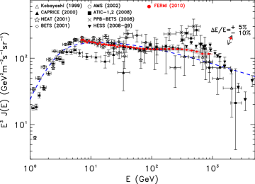
The rise in the fraction in the PAMELA data may have its roots in the astrophysical objects such as nearby pulsars, Monogem at a distance of pc, and Geminga at a distance of pc. Both are nearby objects to Earth which can contribute significantly to the flux, and can match both the PAMELA and Fermi-LAT data sets, see Grasso et al. (2009). A dark matter interpretation of these data sets requires an ad-hoc assumption on the leptohilic nature of the WIMP with an annihilation cross-section , more than orders of magnitude enhancement from thermally produced WIMPS at the TeV scale, se Eq. (206). Such an enhancement in the cross-section is possible at low energies and with low velocities of dark matter provided that the range of the interaction responsible for annihilation is much shorter than the long-range attractive potential, known as a Sommerfeld enhancement Arkani-Hamed et al. (2009), see for a detailed derivation Slatyer (2010) in the mass range of GeV Grasso et al. (2009). It is also possible to conceive a scenario of non-thermal dark matter production in order to evade the strict bound on cross-section, or decaying dark matter scenarios, i.e. Fairbairn and Zupan (2009); Arvanitaki et al. (2009).
Finally, one would also expect a gamma ray signal from the galactic center, the typical signature for a WIMP annihilation will be a line at the WIMP mass, due to the 2s, or production channels. The Fermi-LAT collaboration has released a diffused galactic and extra galactic -ray background Abdo et al. (2010b), however no lines were observed yet Abdo et al. (2010a).
The high energy neutrinos are being another frontier for the indirect dark matter searches as the construction of new experiment IceCube with large volume is underway, in which case even Earth could be used as a detector to study the nature of dark matter, e.g. Albuquerque et al. (2004), or neutrino emission from the passage of Q-balls Kusenko and Shoemaker (2009). Searching for WIMPs in more than one type of experiments; direct, indirect, and the LHC will be necessary in order to stamp the origin of such elusive particles.
V Acknowledgements
The author would like to thank A. Kusenko for many useful discussions and collaborating at the initial stages of this review. He would also like to thank R. Allahverdi, R. Brandenberger, C. Boehm, A. Chatterjee, P. Dayal, B. Dutta, K. Enqvist, A. Ferrantelli, J. Garcia-Bellido, S. Hotchkiss, K. Kazunori, D. Lyth, S. Nadathur, K. Petraki, N. Sahu, Q. Shafi, and P. Stephens for helpful discussions.
References
- Aalseth et al. (2011) Aalseth, C. E., et al. (CoGeNT), 2011, Phys. Rev. Lett. 106, 131301.
- Abada et al. (2006a) Abada, A., S. Davidson, A. Ibarra, F.-X. Josse-Michaux, M. Losada, et al., 2006a, JHEP 0609, 010.
- Abada et al. (2006b) Abada, A., S. Davidson, F.-X. Josse-Michaux, M. Losada, and A. Riotto, 2006b, JCAP 0604, 004.
- Abazajian et al. (2001) Abazajian, K., G. M. Fuller, and M. Patel, 2001, Phys. Rev. D64, 023501.
- Abazajian and Koushiappas (2006) Abazajian, K., and S. M. Koushiappas, 2006, Phys. Rev. D74, 023527.
- Abazajian et al. (2009) Abazajian, K. N., et al. (SDSS), 2009, Astrophys. J. Suppl. 182, 543.
- Abbott and Sikivie (1983) Abbott, L. F., and P. Sikivie, 1983, Phys. Lett. B120, 133.
- Abdo et al. (2009) Abdo, A. A., et al. (The Fermi LAT), 2009, Phys. Rev. Lett. 102, 181101.
- Abdo et al. (2010a) Abdo, A. A., et al., 2010a, Phys. Rev. Lett. 104, 091302.
- Abdo et al. (2010b) Abdo, A. A., et al. (The Fermi-LAT), 2010b, Phys. Rev. Lett. 104, 101101.
- Abel et al. (1995) Abel, S. A., S. Sarkar, and P. L. White, 1995, Nucl. Phys. B454, 663.
- Ackermann et al. (2010) Ackermann, M., et al. (Fermi LAT), 2010, Phys. Rev. D82, 092004.
- Adler (1969) Adler, S. L., 1969, Phys.Rev. 177, 2426.
- Adriani et al. (2009) Adriani, O., et al. (PAMELA), 2009, Nature 458, 607.
- Adriani et al. (2010) Adriani, O., et al. (PAMELA), 2010, Phys. Rev. Lett. 105, 121101.
- Affleck and Dine (1985) Affleck, I., and M. Dine, 1985, Nucl. Phys. B249, 361.
- Aguilar et al. (2001) Aguilar, A., et al. (LSND), 2001, Phys. Rev. D64, 112007.
- Aguilar-Arevalo et al. (2010) Aguilar-Arevalo, A. A., et al. (The MiniBooNE), 2010, Phys. Rev. Lett. 105, 181801.
- Aharonian et al. (2008) Aharonian, F., et al. (H.E.S.S.), 2008, Phys. Rev. Lett. 101, 261104.
- Aharonian et al. (2009) Aharonian, F., et al. (H.E.S.S.), 2009, Astron. Astrophys. 508, 561.
- Ahlers et al. (2006) Ahlers, M., J. Kersten, and A. Ringwald, 2006, JCAP 0607, 005.
- Ahmed et al. (2010) Ahmed, Z., et al. (The CDMS-II), 2010, Science 327, 1619.
- Akhmedov et al. (2003) Akhmedov, E. K., M. Frigerio, and A. Y. Smirnov, 2003, JHEP 09, 021.
- Alam et al. (1995) Alam, M. S., et al. (CLEO), 1995, Phys. Rev. Lett. 74, 2885.
- Albrecht et al. (1982) Albrecht, A. J., P. J. Steinhardt, M. S. Turner, and F. Wilczek, 1982, Phys. Rev. Lett. 48, 1437.
- Albuquerque et al. (2004) Albuquerque, I., G. Burdman, and Z. Chacko, 2004, Phys. Rev. Lett. 92, 221802.
- Albuquerque et al. (2007) Albuquerque, I. F. M., G. Burdman, and Z. Chacko, 2007, Phys. Rev. D75, 035006.
- Allahverdi (2000) Allahverdi, R., 2000, Phys. Rev. D62, 063509.
- Allahverdi et al. (2010a) Allahverdi, R., R. Brandenberger, F.-Y. Cyr-Racine, and A. Mazumdar, 2010a, eprint 1001.2600.
- Allahverdi and Drees (2002) Allahverdi, R., and M. Drees, 2002, Phys. Rev. D66, 063513.
- Allahverdi et al. (2003) Allahverdi, R., B. Dutta, and A. Mazumdar, 2003, Phys. Rev. D67, 123515.
- Allahverdi et al. (2007a) Allahverdi, R., B. Dutta, and A. Mazumdar, 2007a, Phys. Rev. D75, 075018.
- Allahverdi et al. (2007b) Allahverdi, R., B. Dutta, and A. Mazumdar, 2007b, Phys. Rev. Lett. 99, 261301.
- Allahverdi et al. (2008) Allahverdi, R., B. Dutta, and A. Mazumdar, 2008, Phys. Rev. D78, 063507.
- Allahverdi et al. (2011a) Allahverdi, R., B. Dutta, and R. N. Mohapatra, 2011a, Phys. Lett. B695, 181.
- Allahverdi et al. (2010b) Allahverdi, R., B. Dutta, and Y. Santoso, 2010b, Phys. Lett. B687, 225.
- Allahverdi et al. (2010c) Allahverdi, R., B. Dutta, and Y. Santoso, 2010c, Phys.Rev. D82, 035012.
- Allahverdi et al. (2007c) Allahverdi, R., K. Enqvist, J. Garcia-Bellido, A. Jokinen, and A. Mazumdar, 2007c, JCAP 0706, 019.
- Allahverdi et al. (2006) Allahverdi, R., K. Enqvist, J. Garcia-Bellido, and A. Mazumdar, 2006, Phys. Rev. Lett. 97, 191304.
- Allahverdi et al. (2002) Allahverdi, R., K. Enqvist, and A. Mazumdar, 2002, Phys. Rev. D65, 103519.
- Allahverdi et al. (2011b) Allahverdi, R., A. Ferrantelli, J. Garcia-Bellido, and A. Mazumdar, 2011b, eprint 1103.2123.
- Allahverdi et al. (2007d) Allahverdi, R., A. R. Frey, and A. Mazumdar, 2007d, Phys. Rev. D76, 026001.
- Allahverdi et al. (2007e) Allahverdi, R., A. Kusenko, and A. Mazumdar, 2007e, JCAP 0707, 018.
- Allahverdi and Mazumdar (2003) Allahverdi, R., and A. Mazumdar, 2003, Phys. Rev. D67, 023509.
- Allahverdi and Mazumdar (2005) Allahverdi, R., and A. Mazumdar, 2005, eprint hep-ph/0505050.
- Allahverdi and Mazumdar (2006a) Allahverdi, R., and A. Mazumdar, 2006a, eprint hep-ph/0610069.
- Allahverdi and Mazumdar (2006b) Allahverdi, R., and A. Mazumdar, 2006b, JCAP 0610, 008.
- Allahverdi and Mazumdar (2007a) Allahverdi, R., and A. Mazumdar, 2007a, JCAP 0708, 023.
- Allahverdi and Mazumdar (2007b) Allahverdi, R., and A. Mazumdar, 2007b, Phys. Rev. D76, 103526.
- Allahverdi and Mazumdar (2008) Allahverdi, R., and A. Mazumdar, 2008, Phys. Rev. D78, 043511.
- Allen (1988) Allen, B., 1988, Phys. Rev. D37, 2078.
- Ambjorn et al. (1990) Ambjorn, J., T. Askgaard, H. Porter, and M. Shaposhnikov, 1990, Phys.Lett. B244, 479.
- Anderson and Hall (1992) Anderson, G. W., and L. J. Hall, 1992, Phys. Rev. D45, 2685.
- Antusch et al. (2009a) Antusch, S., M. Bastero-Gil, K. Dutta, S. F. King, and P. M. Kostka, 2009a, JCAP 0901, 040.
- Antusch et al. (2009b) Antusch, S., K. Dutta, and P. M. Kostka, 2009b, Phys. Lett. B677, 221.
- Aprile et al. (2011) Aprile, E., et al. (XENON100), 2011, eprint 1104.2549.
- Arafune et al. (2000) Arafune, J., T. Yoshida, S. Nakamura, and K. Ogure, 2000, Phys.Rev. D62, 105013.
- Archambault et al. (2009) Archambault, S., et al., 2009, Phys. Lett. B682, 185.
- Arina and Fornengo (2007) Arina, C., and N. Fornengo, 2007, JHEP 11, 029.
- Arkani-Hamed et al. (2000) Arkani-Hamed, N., S. Dimopoulos, N. Kaloper, and J. March-Russell, 2000, Nucl. Phys. B567, 189.
- Arkani-Hamed et al. (2009) Arkani-Hamed, N., D. P. Finkbeiner, T. R. Slatyer, and N. Weiner, 2009, Phys. Rev. D79, 015014.
- Armendariz-Picon et al. (1999) Armendariz-Picon, C., T. Damour, and V. F. Mukhanov, 1999, Phys. Lett. B458, 209.
- Armengaud et al. (2011) Armengaud, et al. (EDELWEISS), 2011, eprint 1103.4070.
- Arnold et al. (1997) Arnold, P. B., D. Son, and L. G. Yaffe, 1997, Phys.Rev. D55, 6264.
- Arvanitaki et al. (2009) Arvanitaki, A., et al., 2009, Phys. Rev. D80, 055011.
- Asaka et al. (2005) Asaka, T., S. Blanchet, and M. Shaposhnikov, 2005, Phys. Lett. B631, 151.
- Asaka et al. (2000a) Asaka, T., M. Fujii, K. Hamaguchi, and T. Yanagida, 2000a, Phys.Rev. D62, 123514.
- Asaka et al. (1999) Asaka, T., K. Hamaguchi, M. Kawasaki, and T. Yanagida, 1999, Phys. Lett. B464, 12.
- Asaka et al. (2000b) Asaka, T., K. Hamaguchi, M. Kawasaki, and T. Yanagida, 2000b, Phys. Rev. D61, 083512.
- Baacke et al. (1998) Baacke, J., K. H. , and C. Patzold, 1998, Phys. Rev. D58, 125013.
- Balazs et al. (2005) Balazs, C., M. S. Carena, A. Menon, D. E. Morrissey, and C. E. M. Wagner, 2005, Phys. Rev. D71, 075002.
- Balazs et al. (2004) Balazs, C., M. S. Carena, and C. E. M. Wagner, 2004, Phys. Rev. D70, 015007.
- Barate et al. (2003) Barate, R., et al. (LEP Working Group for Higgs boson searches), 2003, Phys. Lett. B565, 61.
- Barbier et al. (2005) Barbier, R., et al., 2005, Phys. Rept. 420, 1.
- Bastero-Gil et al. (2002) Bastero-Gil, M., E. J. Copeland, J. Gray, A. Lukas, and M. Plumacher, 2002, Phys. Rev. D66, 066005.
- Bastero-Gil et al. (2003) Bastero-Gil, M., V. Di Clemente, and S. F. King, 2003, Phys. Rev. D67, 083504.
- Bastero-Gil and King (1998) Bastero-Gil, M., and S. F. King, 1998, Phys. Lett. B423, 27.
- Bastero-Gil and King (1999) Bastero-Gil, M., and S. F. King, 1999, Nucl. Phys. B549, 391.
- Becker et al. (2005) Becker, K., M. Becker, and A. Krause, 2005, Nucl. Phys. B715, 349.
- Begeman et al. (1991) Begeman, K., A. Broeils, and R. Sanders, 1991, Mon.Not.Roy.Astron.Soc. 249, 523.
- Behnke et al. (2011) Behnke, E., et al., 2011, Phys. Rev. Lett. 106, 021303.
- Bell and Jackiw (1969) Bell, J., and R. Jackiw, 1969, Nuovo Cim. A60, 47.
- Beltran et al. (2007) Beltran, M., J. Garcia-Bellido, and J. Lesgourgues, 2007, Phys. Rev. D75, 103507.
- Beltran et al. (2004) Beltran, M., J. Garcia-Bellido, J. Lesgourgues, and A. Riazuelo, 2004, Phys. Rev. D70, 103530.
- Ben-Dayan and Brustein (2010) Ben-Dayan, I., and R. Brustein, 2010, JCAP 1009, 007.
- Bennett et al. (2004) Bennett, G. W., et al. (Muon g-2), 2004, Phys. Rev. Lett. 92, 161802.
- Bento and Berezhiani (2001) Bento, L., and Z. Berezhiani, 2001, Phys. Rev. Lett. 87, 231304.
- Berezhiani et al. (2001) Berezhiani, Z., A. Mazumdar, and A. Perez-Lorenzana, 2001, Phys. Lett. B518, 282.
- Berg et al. (2005a) Berg, M., M. Haack, and B. Kors, 2005a, Phys. Rev. D71, 026005.
- Berg et al. (2005b) Berg, M., M. Haack, and B. Kors, 2005b, JHEP 11, 030.
- Berg et al. (2006) Berg, M., M. Haack, and B. Kors, 2006, Phys. Rev. Lett. 96, 021601.
- Berger et al. (2008) Berger, C. F., L. Covi, S. Kraml, and F. Palorini, 2008, JCAP 0810, 005.
- Bergstrom et al. (1998) Bergstrom, L., P. Ullio, and J. H. Buckley, 1998, Astropart. Phys. 9, 137.
- Bernabei et al. (2004) Bernabei, R., et al., 2004, Int. J. Mod. Phys. D13, 2127.
- Bernabei et al. (2008) Bernabei, R., et al. (DAMA), 2008, Eur. Phys. J. C56, 333.
- Bernabei et al. (2010) Bernabei, R., et al., 2010, Eur. Phys. J. C67, 39.
- Bertolami and Ross (1987) Bertolami, O., and G. G. Ross, 1987, Phys. Lett. B183, 163.
- Bertone et al. (2005) Bertone, G., D. Hooper, and J. Silk, 2005, Phys. Rept. 405, 279.
- Bertschinger (2006) Bertschinger, E., 2006, Phys. Rev. D74, 063509.
- Bevis et al. (2008) Bevis, N., M. Hindmarsh, M. Kunz, and J. Urrestilla, 2008, Phys. Rev. Lett. 100, 021301.
- Bezrukov and Shaposhnikov (2008) Bezrukov, F. L., and M. Shaposhnikov, 2008, Phys. Lett. B659, 703.
- Binétruy and Dvali (1996) Binétruy, P., and G. R. Dvali, 1996, Phys. Lett. B388, 241.
- Binetruy et al. (1984) Binetruy, P., G. Girardi, and P. Salati, 1984, Nucl.Phys. B237, 285.
- Bird et al. (2008) Bird, C., K. Koopmans, and M. Pospelov, 2008, Phys. Rev. D78, 083010.
- Birrell and Davies (1982) Birrell, N. D., and P. C. W. Davies, 1982, cambridge, Uk: Univ. Pr. 340p.
- Biswas et al. (2010) Biswas, T., T. Koivisto, and A. Mazumdar, 2010, JCAP 1011, 008.
- Biswas and Mazumdar (2009) Biswas, T., and A. Mazumdar, 2009, eprint 0901.4930.
- Biswas et al. (2006) Biswas, T., A. Mazumdar, and W. Siegel, 2006, JCAP 0603, 009.
- Bochkarev and Shaposhnikov (1987) Bochkarev, A., and M. Shaposhnikov, 1987, Mod.Phys.Lett. A2, 417.
- Bochkarev et al. (1991) Bochkarev, A. I., S. V. Kuzmin, and M. E. Shaposhnikov, 1991, Phys. Rev. D43, 369.
- Bode et al. (2001) Bode, P., J. P. Ostriker, and N. Turok, 2001, Astrophys. J. 556, 93.
- Bolton et al. (2006) Bolton, A. S., S. Burles, L. V. E. Koopmans, T. Treu, and L. A. Moustakas, 2006, Astrophys. J. 638, 703.
- Bolz et al. (2001) Bolz, M., A. Brandenburg, and W. Buchmuller, 2001, Nucl. Phys. B606, 518.
- Bond and Szalay (1983) Bond, J. R., and A. S. Szalay, 1983, Astrophys. J. 274, 443.
- Borde et al. (2003) Borde, A., A. H. Guth, and A. Vilenkin, 2003, Phys. Rev. Lett. 90, 151301.
- Borde and Vilenkin (1994) Borde, A., and A. Vilenkin, 1994, Phys. Rev. Lett. 72, 3305.
- Brandenberger and Kung (1990) Brandenberger, R. H., and J. H. Kung, 1990, Phys. Rev. D42, 1008.
- Brandenburg and Steffen (2004) Brandenburg, A., and F. D. Steffen, 2004, JCAP 0408, 008.
- Brax and Martin (2005) Brax, P., and J. Martin, 2005, Phys. Rev. D72, 023518.
- Buchmueller et al. (2011) Buchmueller, O., et al., 2011, Eur. Phys. J. C71, 1634.
- Buchmuller et al. (2002) Buchmuller, W., P. Di Bari, and M. Plumacher, 2002, Nucl.Phys. B643, 367.
- Buchmuller et al. (2003) Buchmuller, W., P. Di Bari, and M. Plumacher, 2003, Nucl. Phys. B665, 445.
- Buchmuller et al. (2005a) Buchmuller, W., P. Di Bari, and M. Plumacher, 2005a, Ann. Phys. 315, 305.
- Buchmuller et al. (2005b) Buchmuller, W., R. D. Peccei, and T. Yanagida, 2005b, Ann. Rev. Nucl. Part. Sci. 55, 311.
- Buchmuller and Plumacher (1998) Buchmuller, W., and M. Plumacher, 1998, Phys. Lett. B431, 354.
- Buchmuller and Plumacher (2000) Buchmuller, W., and M. Plumacher, 2000, Int. J. Mod. Phys. A15, 5047.
- Bueno Sanchez et al. (2007) Bueno Sanchez, J. C., K. Dimopoulos, and D. H. Lyth, 2007, JCAP 0701, 015.
- Bustamante et al. (2009) Bustamante, M., L. Cieri, and J. Ellis, 2009, eprint 0911.4409.
- Carena et al. (2003) Carena, M. S., M. Quiros, M. Seco, and C. Wagner, 2003, Nucl.Phys. B650, 24.
- Carena et al. (1996) Carena, M. S., M. Quiros, and C. Wagner, 1996, Phys.Lett. B380, 81.
- Carr (1975) Carr, B. J., 1975, Astrophys. J. 201, 1.
- Carr and Hawking (1974) Carr, B. J., and S. W. Hawking, 1974, Mon. Not. Roy. Astron. Soc. 168, 399.
- Carr et al. (2010) Carr, B. J., K. Kohri, Y. Sendouda, and J. Yokoyama, 2010, Phys. Rev. D81, 104019.
- Carr and Lidsey (1993) Carr, B. J., and J. E. Lidsey, 1993, Phys. Rev. D48, 543.
- Carson et al. (1990) Carson, L., X. Li, L. D. McLerran, and R.-T. Wang, 1990, Phys.Rev. D42, 2127.
- Casas and Munoz (1993) Casas, J. A., and C. Munoz, 1993, Phys. Lett. B306, 288.
- Chang et al. (2008) Chang, J., et al., 2008, Nature 456, 362.
- Chatterjee and Mazumdar (2011) Chatterjee, A., and A. Mazumdar, 2011, eprint 1103.5758.
- Choi et al. (2008) Choi, K.-Y., L. Roszkowski, and R. Ruiz de Austri, 2008, JHEP 04, 016.
- Chung et al. (2001) Chung, D. J. H., P. Crotty, E. W. Kolb, and A. Riotto, 2001, Phys. Rev. D64, 043503.
- Chung et al. (2009) Chung, D. J. H., B. Garbrecht, M. J. Ramsey-Musolf, and S. Tulin, 2009, Phys. Rev. Lett. 102, 061301.
- Chung et al. (1999a) Chung, D. J. H., E. W. Kolb, and A. Riotto, 1999a, Phys. Rev. D60, 063504.
- Chung et al. (1999b) Chung, D. J. H., E. W. Kolb, and A. Riotto, 1999b, Phys. Rev. D59, 023501.
- Chung et al. (2000) Chung, D. J. H., E. W. Kolb, A. Riotto, and I. I. Tkachev, 2000, Phys. Rev. D62, 043508.
- Chung et al. (2005) Chung, D. J. H., et al., 2005, Phys. Rept. 407, 1.
- Chuzhoy and Kolb (2009) Chuzhoy, L., and E. W. Kolb, 2009, JCAP 0907, 014.
- Cicoli and Mazumdar (2010a) Cicoli, M., and A. Mazumdar, 2010a, eprint 1010.0941.
- Cicoli and Mazumdar (2010b) Cicoli, M., and A. Mazumdar, 2010b, JCAP 1009, 025.
- Clesse and Rocher (2008) Clesse, S., and J. Rocher, 2008, eprint 0809.4355.
- Cline et al. (1998) Cline, J. M., M. Joyce, and K. Kainulainen, 1998, Phys.Lett. B417, 79.
- Cline et al. (2000) Cline, J. M., M. Joyce, and K. Kainulainen, 2000, JHEP 0007, 018, erratum added online, Oct/2/2001.
- Cline and Raby (1991) Cline, J. M., and S. Raby, 1991, Phys. Rev. D43, 1781.
- Cline and Stoica (2005) Cline, J. M., and H. Stoica, 2005, Phys. Rev. D72, 126004.
- Clowe et al. (2006) Clowe, D., et al., 2006, Astrophys. J. 648, L109.
- Cohen et al. (1993) Cohen, A. G., D. Kaplan, and A. Nelson, 1993, Ann.Rev.Nucl.Part.Sci. 43, 27.
- Coleman (1985) Coleman, S. R., 1985, Nucl.Phys. B262, 263.
- Coleman and Weinberg (1973) Coleman, S. R., and E. J. Weinberg, 1973, Phys. Rev. D7, 1888.
- Copeland et al. (2001) Copeland, E. J., A. R. Liddle, and J. E. Lidsey, 2001, Phys. Rev. D64, 023509.
- Copeland et al. (1994) Copeland, E. J., A. R. Liddle, D. H. Lyth, E. D. Stewart, and D. Wands, 1994, Phys. Rev. D49, 6410.
- Copeland et al. (1999) Copeland, E. J., A. Mazumdar, and N. J. Nunes, 1999, Phys. Rev. D60, 083506.
- Copi et al. (1999) Copi, C. J., J. Heo, and L. M. Krauss, 1999, Phys. Lett. B461, 43.
- Cornwall et al. (2001) Cornwall, J. M., D. Grigoriev, and A. Kusenko, 2001, Phys. Rev. D64, 123518.
- Cornwall and Kusenko (2000) Cornwall, J. M., and A. Kusenko, 2000, Phys. Rev. D61, 103510.
- Covi et al. (2001) Covi, L., H.-B. Kim, J. E. Kim, and L. Roszkowski, 2001, JHEP 05, 033.
- Covi et al. (1996) Covi, L., E. Roulet, and F. Vissani, 1996, Phys. Lett. B384, 169.
- Cyburt et al. (2003) Cyburt, R. H., J. R. Ellis, B. D. Fields, and K. A. Olive, 2003, Phys. Rev. D67, 103521.
- Cyburt et al. (2008) Cyburt, R. H., B. D. Fields, and K. A. Olive, 2008, JCAP 0811, 012.
- D’Ambrosio et al. (2003) D’Ambrosio, G., G. F. Giudice, and M. Raidal, 2003, Phys. Lett. B575, 75.
- Damour and Mukhanov (1998) Damour, T., and V. F. Mukhanov, 1998, Phys. Rev. Lett. 80, 3440.
- Dave et al. (2001) Dave, R., D. N. Spergel, P. J. Steinhardt, and B. D. Wandelt, 2001, Astrophys. J. 547, 574.
- Davidson and Ibarra (2002) Davidson, S., and A. Ibarra, 2002, Phys. Lett. B535, 25.
- Davidson et al. (2008) Davidson, S., E. Nardi, and Y. Nir, 2008, Phys. Rept. 466, 105.
- Davidson and Sarkar (2000) Davidson, S., and S. Sarkar, 2000, JHEP 11, 012.
- De Rujula et al. (1990) De Rujula, A., S. L. Glashow, and U. Sarid, 1990, Nucl. Phys. B333, 173.
- Diaz-Cruz et al. (2007) Diaz-Cruz, J. L., J. R. Ellis, K. A. Olive, and Y. Santoso, 2007, JHEP 05, 003.
- Dick et al. (2000) Dick, K., M. Lindner, M. Ratz, and D. Wright, 2000, Phys. Rev. Lett. 84, 4039.
- Dimopoulos et al. (1990) Dimopoulos, S., D. Eichler, R. Esmailzadeh, and G. D. Starkman, 1990, Phys. Rev. D41, 2388.
- Dimopoulos and Hall (1988) Dimopoulos, S., and L. J. Hall, 1988, Phys. Lett. B207, 210.
- Dimopoulos et al. (2005) Dimopoulos, S., S. Kachru, J. McGreevy, and J. G. Wacker, 2005, eprint hep-th/0507205.
- Dine and Fischler (1983) Dine, M., and W. Fischler, 1983, Phys. Lett. B120, 137.
- Dine et al. (1984) Dine, M., W. Fischler, and D. Nemeschansky, 1984, Phys. Lett. B136, 169.
- Dine et al. (1981) Dine, M., W. Fischler, and M. Srednicki, 1981, Phys. Lett. B104, 199.
- Dine and Kusenko (2004) Dine, M., and A. Kusenko, 2004, Rev. Mod. Phys. 76, 1.
- Dine et al. (1992) Dine, M., R. G. Leigh, P. Huet, A. D. Linde, and D. A. Linde, 1992, Phys.Lett. B283, 319.
- Dine et al. (1996a) Dine, M., A. E. Nelson, Y. Nir, and Y. Shirman, 1996a, Phys. Rev. D53, 2658.
- Dine et al. (1995a) Dine, M., A. E. Nelson, and Y. Shirman, 1995a, Phys.Rev. D51, 1362.
- Dine et al. (1995b) Dine, M., L. Randall, and S. D. Thomas, 1995b, Phys. Rev. Lett. 75, 398.
- Dine et al. (1996b) Dine, M., L. Randall, and S. D. Thomas, 1996b, Nucl. Phys. B458, 291.
- Dodelson (2003) Dodelson, S., 2003, amsterdam, Netherlands: Academic Pr. (2003) 440 p.
- Dodelson et al. (2006) Dodelson, S., A. Melchiorri, and A. Slosar, 2006, Phys. Rev. Lett. 97, 04301.
- Dodelson and Widrow (1994) Dodelson, S., and L. M. Widrow, 1994, Phys. Rev. Lett. 72, 17.
- Dolgov (1992) Dolgov, A. D., 1992, Phys. Rept. 222, 309.
- Dolgov and Hansen (2002) Dolgov, A. D., and S. H. Hansen, 2002, Astropart. Phys. 16, 339.
- Dolgov and Kirilova (1990) Dolgov, A. D., and D. P. Kirilova, 1990, Sov. J. Nucl. Phys. 51, 172.
- Drees and Erfani (2011) Drees, M., and E. Erfani, 2011, eprint 1102.2340.
- Drees and Tata (1990) Drees, M., and X. Tata, 1990, Phys. Lett. B252, 695.
- Dressler et al. (1987) Dressler, A., et al., 1987, Astrophys. J. 313, L37.
- Drukier et al. (1986) Drukier, A. K., K. Freese, and D. N. Spergel, 1986, Phys. Rev. D33, 3495.
- Dvali et al. (1998) Dvali, G. R., A. Kusenko, and M. E. Shaposhnikov, 1998, Phys. Lett. B417, 99.
- Dvali et al. (1994) Dvali, G. R., Q. Shafi, and R. K. Schaefer, 1994, Phys. Rev. Lett. 73, 1886.
- Edsjo and Gondolo (1997) Edsjo, J., and P. Gondolo, 1997, Phys.Rev. D56, 1879.
- Ellis et al. (1982) Ellis, J. R., S. Ferrara, and D. V. Nanopoulos, 1982, Phys.Lett. B114, 231.
- Ellis et al. (1984a) Ellis, J. R., J. S. Hagelin, D. V. Nanopoulos, K. A. Olive, and M. Srednicki, 1984a, Nucl. Phys. B238, 453.
- Ellis et al. (1984b) Ellis, J. R., J. E. Kim, and D. V. Nanopoulos, 1984b, Phys. Lett. B145, 181.
- Ellis et al. (2008) Ellis, J. R., K. A. Olive, and Y. Santoso, 2008, JHEP 10, 005.
- Ellis et al. (2006) Ellis, J. R., A. R. Raklev, and O. K. Oye, 2006, JHEP 10, 061.
- Elmfors et al. (1994) Elmfors, P., K. Enqvist, and I. Vilja, 1994, Phys.Lett. B326, 37.
- Enqvist and Eskola (1990) Enqvist, K., and K. Eskola, 1990, Mod.Phys.Lett. A5, 1919.
- Enqvist et al. (2000) Enqvist, K., A. Jokinen, and J. McDonald, 2000, Phys.Lett. B483, 191.
- Enqvist et al. (2002a) Enqvist, K., S. Kasuya, and A. Mazumdar, 2002a, Phys. Rev. D66, 043505.
- Enqvist et al. (2002b) Enqvist, K., S. Kasuya, and A. Mazumdar, 2002b, Phys. Rev. Lett. 89, 091301.
- Enqvist et al. (2004a) Enqvist, K., S. Kasuya, and A. Mazumdar, 2004a, Phys. Rev. Lett. 93, 061301.
- Enqvist and Mazumdar (2003) Enqvist, K., and A. Mazumdar, 2003, Phys. Rept. 380, 99.
- Enqvist et al. (2004b) Enqvist, K., A. Mazumdar, and A. Perez-Lorenzana, 2004b, Phys. Rev. D70, 103508.
- Enqvist et al. (2010a) Enqvist, K., A. Mazumdar, and P. Stephens, 2010a, JCAP 1006, 020.
- Enqvist and McDonald (1998) Enqvist, K., and J. McDonald, 1998, Phys.Lett. B425, 309.
- Enqvist and McDonald (1999) Enqvist, K., and J. McDonald, 1999, Nucl.Phys. B538, 321.
- Enqvist and McDonald (2000) Enqvist, K., and J. McDonald, 2000, Nucl.Phys. B570, 407.
- Enqvist and Sirkka (1993) Enqvist, K., and J. Sirkka, 1993, Phys. Lett. B314, 298.
- Enqvist et al. (2010b) Enqvist, K., P. Stephens, O. Taanila, and A. Tranberg, 2010b, JCAP 1009, 019.
- Fairbairn and Zupan (2009) Fairbairn, M., and J. Zupan, 2009, JCAP 0907, 001.
- Fayet (1979) Fayet, P., 1979, Phys. Lett. B86, 272.
- Felder et al. (2001) Felder, G. N., et al., 2001, Phys. Rev. Lett. 87, 011601.
- Feng and Moroi (1998) Feng, J. L., and T. Moroi, 1998, Phys. Rev. D58, 035001.
- Feng et al. (2004) Feng, J. L., S. Su, and F. Takayama, 2004, Phys. Rev. D70, 075019.
- Fields and Sarkar (2006) Fields, B., and S. Sarkar, 2006, eprint astro-ph/0601514.
- Flanz et al. (1995) Flanz, M., E. A. Paschos, and U. Sarkar, 1995, Phys. Lett. B345, 248.
- Flores et al. (2007) Flores, R. A., et al., 2007, Mon. Not. Roy. Astron. Soc. 377, 883.
- Fogli et al. (2008) Fogli, G. L., et al., 2008, Phys. Rev. D78, 033010.
- Freese et al. (1988) Freese, K., J. A. Frieman, and A. Gould, 1988, Phys. Rev. D37, 3388.
- Freese et al. (1990) Freese, K., J. A. Frieman, and A. V. Olinto, 1990, Phys. Rev. Lett. 65, 3233.
- Frey et al. (2006) Frey, A. R., A. Mazumdar, and R. C. Myers, 2006, Phys. Rev. D73, 026003.
- Fryer and Kusenko (2006) Fryer, C. L., and A. Kusenko, 2006, Astrophys. J. Suppl. 163, 335.
- Fujii and Hamaguchi (2002) Fujii, M., and K. Hamaguchi, 2002, Phys.Rev. D66, 083501.
- Fukugita and Yanagida (1986) Fukugita, M., and T. Yanagida, 1986, Phys. Lett. B174, 45.
- Garcia-Bellido et al. (1999) Garcia-Bellido, J., D. Y. Grigoriev, A. f, and M. E. Shaposhnikov, 1999, Phys. Rev. D60, 123504.
- Garcia-Bellido and Linde (1998) Garcia-Bellido, J., and A. D. Linde, 1998, Phys. Rev. D57, 6075.
- Gell-Mann and Slansky (1980) Gell-Mann, R., M. Ramond, and S. Slansky, 1980, supergravity (P. van Nieuwenhuizen et al. eds.), North Holland, Amsterdam, p. 315.
- Gentile et al. (2004) Gentile, G., P. Salucci, U. Klein, D. Vergani, and P. Kalberla, 2004, Mon. Not. Roy. Astron. Soc. 351, 903.
- Gherghetta et al. (1996) Gherghetta, T., C. F. Kolda, and S. P. Martin, 1996, Nucl. Phys. B468, 37.
- Ghez et al. (1998) Ghez, A., B. Klein, M. Morris, and E. Becklin, 1998, Astrophys.J. 509, 678, * Fermilab Library Only *.
- Giudice and Masiero (1988) Giudice, G. F., and A. Masiero, 1988, Phys. Lett. B206, 480.
- Giudice et al. (2004) Giudice, G. F., A. Notari, M. Raidal, A. Riotto, and A. Strumia, 2004, Nucl. Phys. B685, 89.
- Giudice et al. (1999a) Giudice, G. F., M. Peloso, A. Riotto, and I. Tkachev, 1999a, JHEP 08, 014.
- Giudice and Rattazzi (1999) Giudice, G. F., and R. Rattazzi, 1999, Phys. Rept. 322, 419.
- Giudice et al. (1999b) Giudice, G. F., A. Riotto, and I. Tkachev, 1999b, JHEP 11, 036.
- Goldberg (1983) Goldberg, H., 1983, Phys. Rev. Lett. 50, 1419.
- Gondolo et al. (2004) Gondolo, P., et al., 2004, JCAP 0407, 008.
- Gonzalez-Garcia et al. (2010) Gonzalez-Garcia, M. C., M. Maltoni, and J. Salvado, 2010, JHEP 04, 056.
- Goodman and Witten (1985) Goodman, M. W., and E. Witten, 1985, Phys. Rev. D31, 3059.
- Grasso et al. (2009) Grasso, D., et al. (FERMI-LAT), 2009, Astropart. Phys. 32, 140.
- Green et al. (2004) Green, A. M., S. Hofmann, and D. J. Schwarz, 2004, Mon. Not. Roy. Astron. Soc. 353, L23.
- Green et al. (2005) Green, A. M., S. Hofmann, and D. J. Schwarz, 2005, JCAP 0508, 003.
- Green and Liddle (1997) Green, A. M., and A. R. Liddle, 1997, Phys. Rev. D56, 6166.
- Green and Liddle (1999) Green, A. M., and A. R. Liddle, 1999, Phys. Rev. D60, 063509.
- Green and Lidsey (2000) Green, A. M., and J. E. Lidsey, 2000, Phys. Rev. D61, 067301.
- Green and Malik (2001) Green, A. M., and K. A. Malik, 2001, Phys. Rev. D64, 021301.
- Green and Mazumdar (2002) Green, A. M., and A. Mazumdar, 2002, Phys. Rev. D65, 105022.
- Greene and Kofman (1999) Greene, P. B., and L. Kofman, 1999, Phys. Lett. B448, 6.
- Greene and Kofman (2000) Greene, P. B., and L. Kofman, 2000, Phys. Rev. D62, 123516.
- Griest and Kamionkowski (1990) Griest, K., and M. Kamionkowski, 1990, Phys. Rev. Lett. 64, 615.
- Griest and Seckel (1991) Griest, K., and D. Seckel, 1991, Phys. Rev. D43, 3191.
- Grisaru et al. (1979) Grisaru, M. T., W. Siegel, and M. Rocek, 1979, Nucl. Phys. B159, 429.
- Grishchuk (1975) Grishchuk, L. P., 1975, Sov. Phys. JETP 40, 409.
- Grishchuk and Sidorov (1989) Grishchuk, L. P., and Y. V. Sidorov, 1989, Class. Quant. Grav. 6, L161.
- Grojean et al. (2005) Grojean, C., G. Servant, and J. D. Wells, 2005, Phys. Rev. D71, 036001.
- Grossman et al. (2003) Grossman, Y., T. Kashti, Y. Nir, and E. Roulet, 2003, Phys. Rev. Lett. 91, 251801.
- Grossman et al. (2004) Grossman, Y., T. Kashti, Y. Nir, and E. Roulet, 2004, JHEP 11, 080.
- Grossman et al. (2005) Grossman, Y., R. Kitano, and H. Murayama, 2005, JHEP 06, 058.
- Guth (1981) Guth, A. H., 1981, Phys. Rev. D23, 347.
- Haber and Kane (1985) Haber, H. E., and G. L. Kane, 1985, Phys. Rept. 117, 75.
- Halyo (1996) Halyo, E., 1996, Phys. Lett. B387, 43.
- Hamaguchi et al. (2007) Hamaguchi, K., T. Hatsuda, M. Kamimura, Y. Kino, and T. T. Yanagida, 2007, Phys. Lett. B650, 268.
- Hannestad et al. (2010) Hannestad, S., A. Mirizzi, G. G. Raffelt, and Y. Y. Y. Wong, 2010, JCAP 1008, 001.
- Harrison (1970) Harrison, E. R., 1970, Phys. Rev. D1, 2726.
- Harvey and Kolb (1981) Harvey, J. A., and E. W. Kolb, 1981, Phys.Rev. D24, 2090.
- Hawking (1971) Hawking, S., 1971, Mon. Not. Roy. Astron. Soc. 152, 75.
- Hidaka and Fuller (2006) Hidaka, J., and G. M. Fuller, 2006, Phys. Rev. D74, 125015.
- Hidaka and Fuller (2007) Hidaka, J., and G. M. Fuller, 2007, Phys. Rev. D76, 083516.
- Hofmann et al. (2001) Hofmann, S., D. J. Schwarz, and H. Stoecker, 2001, Phys. Rev. D64, 083507.
- ’t Hooft (1976a) ’t Hooft, G., 1976a, Phys.Rev. D14, 3432.
- ’t Hooft (1976b) ’t Hooft, G., 1976b, Phys.Rev.Lett. 37, 8.
- Hotchkiss et al. (2008) Hotchkiss, S., G. German, G. G. Ross, and S. Sarkar, 2008, JCAP 0810, 015.
- Hotchkiss et al. (2011) Hotchkiss, S., A. Mazumdar, and S. Nadathur, 2011, eprint 1101.6046.
- Huet and Nelson (1996) Huet, P., and A. E. Nelson, 1996, Phys.Rev. D53, 4578.
- Hunt and Sarkar (2010) Hunt, P., and S. Sarkar, 2010, Mon. Not. Roy. Astron. Soc. 401, 547.
- Iocco et al. (2009) Iocco, F., G. Mangano, G. Miele, O. Pisanti, and P. D. Serpico, 2009, Phys. Rept. 472, 1.
- Jaikumar and Mazumdar (2004) Jaikumar, P., and A. Mazumdar, 2004, Nucl. Phys. B683, 264.
- Jeannerot (1997) Jeannerot, R., 1997, Phys. Rev. D56, 6205.
- Jeannerot and Postma (2005) Jeannerot, R., and M. Postma, 2005, JHEP 05, 071.
- Jeannerot et al. (2003) Jeannerot, R., J. Rocher, and M. Sakellariadou, 2003, Phys. Rev. D68, 103514.
- Jedamzik and Niemeyer (1999) Jedamzik, K., and J. C. Niemeyer, 1999, Phys. Rev. D59, 124014.
- Jedamzik and Pospelov (2009) Jedamzik, K., and M. Pospelov, 2009, New J. Phys. 11, 105028.
- Jokinen and Mazumdar (2004) Jokinen, A., and A. Mazumdar, 2004, Phys. Lett. B597, 222.
- Jungman et al. (1996) Jungman, G., M. Kamionkowski, and K. Griest, 1996, Phys. Rept. 267, 195.
- Kainulainen et al. (2001) Kainulainen, K., T. Prokopec, M. G. Schmidt, and S. Weinstock, 2001, JHEP 0106, 031.
- Kajantie et al. (1996) Kajantie, K., M. Laine, K. Rummukainen, and M. E. Shaposhnikov, 1996, Phys.Rev.Lett. 77, 2887.
- Kallosh (2008) Kallosh, R., 2008, Lect. Notes Phys. 738, 119.
- Kallosh et al. (2000a) Kallosh, R., L. Kofman, A. D. Linde, and A. Van Proeyen, 2000a, Phys. Rev. D61, 103503.
- Kallosh et al. (2000b) Kallosh, R., L. Kofman, A. D. Linde, and A. Van Proeyen, 2000b, Class. Quant. Grav. 17, 4269.
- Kane et al. (1994) Kane, G. L., C. F. Kolda, L. Roszkowski, and J. D. Wells, 1994, Phys. Rev. D49, 6173.
- Kang et al. (2009) Kang, J., P. Langacker, T. Li, and T. Liu, 2009, eprint 0911.2939.
- Kang et al. (2005) Kang, J., P. Langacker, T.-j. Li, and T. Liu, 2005, Phys. Rev. Lett. 94, 061801.
- Kang et al. (2008) Kang, J., M. A. Luty, and S. Nasri, 2008, JHEP 09, 086.
- Kanti and Olive (1999a) Kanti, P., and K. A. Olive, 1999a, Phys. Lett. B464, 192.
- Kanti and Olive (1999b) Kanti, P., and K. A. Olive, 1999b, Phys. Rev. D60, 043502.
- Kaplinghat et al. (2000) Kaplinghat, M., L. Knox, and M. S. Turner, 2000, Phys. Rev. Lett. 85, 3335.
- Karsch et al. (2001) Karsch, F., E. Laermann, and A. Peikert, 2001, Nucl. Phys. B605, 579.
- Kasuya and Kawasaki (2000a) Kasuya, S., and M. Kawasaki, 2000a, Phys. Rev. D62, 023512.
- Kasuya and Kawasaki (2000b) Kasuya, S., and M. Kawasaki, 2000b, Phys. Rev. D61, 041301.
- Kasuya and Kawasaki (2006) Kasuya, S., and M. Kawasaki, 2006, Phys. Rev. D74, 063507.
- Kawasaki et al. (2005) Kawasaki, M., K. Kohri, and T. Moroi, 2005, Phys. Lett. B625, 7.
- Kawasaki et al. (2008) Kawasaki, M., K. Kohri, T. Moroi, and A. Yotsuyanagi, 2008, Phys. Rev. D78, 065011.
- Kawasaki et al. (2000) Kawasaki, M., M. Yamaguchi, and T. Yanagida, 2000, Phys. Rev. Lett. 85, 3572.
- Kawasaki et al. (2001) Kawasaki, M., M. Yamaguchi, and T. Yanagida, 2001, Phys. Rev. D63, 103514.
- Kessler et al. (2009) Kessler, R., et al., 2009, Astrophys. J. Suppl. 185, 32.
- Khlebnikov and Shaposhnikov (1988) Khlebnikov, S. Y., and M. E. Shaposhnikov, 1988, Nucl. Phys. B308, 885.
- Khlebnikov and Tkachev (1996) Khlebnikov, S. Y., and I. I. Tkachev, 1996, Phys. Rev. Lett. 77, 219.
- Khlebnikov and Tkachev (1997a) Khlebnikov, S. Y., and I. I. Tkachev, 1997a, Phys. Rev. Lett. 79, 1607.
- Khlebnikov and Tkachev (1997b) Khlebnikov, S. Y., and I. I. Tkachev, 1997b, Phys. Lett. B390, 80.
- Kim (1979) Kim, J. E., 1979, Phys. Rev. Lett. 43, 103.
- Kim (1984) Kim, J. E., 1984, Phys. Lett. B136, 378.
- Kim (1987) Kim, J. E., 1987, Phys. Rept. 150, 1.
- Kim and Nilles (1984) Kim, J. E., and H. P. Nilles, 1984, Phys. Lett. B138, 150.
- Kitano et al. (2008) Kitano, R., H. Murayama, and M. Ratz, 2008, Phys. Lett. B669, 145.
- Klinkhamer and Manton (1984) Klinkhamer, F. R., and N. Manton, 1984, Phys.Rev. D30, 2212.
- Klypin et al. (1999) Klypin, A. A., A. V. Kravtsov, O. Valenzuela, and F. Prada, 1999, Astrophys. J. 522, 82.
- Kofman et al. (2002) Kofman, L., A. D. Linde, and V. F. Mukhanov, 2002, JHEP 10, 057.
- Kofman et al. (1994) Kofman, L., A. D. Linde, and A. A. Starobinsky, 1994, Phys. Rev. Lett. 73, 3195.
- Kofman et al. (1997) Kofman, L., A. D. Linde, and A. A. Starobinsky, 1997, Phys. Rev. D56, 3258.
- Kohri et al. (2009) Kohri, K., A. Mazumdar, and N. Sahu, 2009, eprint 0905.1625.
- Kolb and Turner (1988) Kolb, E. ., Edward W., and E. . Turner, Michael S., 1988, redwood city, USA: Addison-Wesley, 719 P. (Frontiers in physics, 70).
- Kolb et al. (1998) Kolb, E. W., D. J. H. Chung, and A. Riotto, 1998, eprint hep-ph/9810361.
- Kolb et al. (1995) Kolb, E. W., J. E. Lidsey, M. Abney, E. J. Copeland, and A. R. Liddle, 1995, Nucl. Phys. Proc. Suppl. 43, 118.
- Komatsu et al. (2009) Komatsu, E., et al. (WMAP), 2009, Astrophys. J. Suppl. 180, 330.
- Komatsu et al. (2011) Komatsu, E., et al. (WMAP), 2011, Astrophys. J. Suppl. 192, 18.
- Kosowsky and Turner (1995) Kosowsky, A., and M. S. Turner, 1995, Phys. Rev. D52, 1739.
- Krauss and Trodden (1999) Krauss, L. M., and M. Trodden, 1999, Phys. Rev. Lett. 83, 1502.
- Kravtsov et al. (1998) Kravtsov, A. V., A. A. Klypin, J. S. Bullock, and J. R. Primack, 1998, Astrophys. J. 502, 48.
- Kusenko (1997a) Kusenko, A., 1997a, Phys.Lett. B404, 285.
- Kusenko (1997b) Kusenko, A., 1997b, Phys.Lett. B405, 108.
- Kusenko (2006) Kusenko, A., 2006, Phys. Rev. Lett. 97, 241301.
- Kusenko (2009) Kusenko, A., 2009, Phys. Rept. 481, 1.
- Kusenko et al. (1998) Kusenko, A., V. Kuzmin, M. E. Shaposhnikov, and P. Tinyakov, 1998, Phys.Rev.Lett. 80, 3185.
- Kusenko et al. (2009) Kusenko, A., A. Mazumdar, and T. Multamaki, 2009, Phys. Rev. D79, 124034.
- Kusenko and Segre (1996) Kusenko, A., and G. Segre, 1996, Phys. Rev. Lett. 77, 4872.
- Kusenko and Segre (1999) Kusenko, A., and G. Segre, 1999, Phys. Rev. D59, 061302.
- Kusenko and Shaposhnikov (1998) Kusenko, A., and M. E. Shaposhnikov, 1998, Phys.Lett. B418, 46.
- Kusenko and Shoemaker (2009) Kusenko, A., and I. M. Shoemaker, 2009, Phys. Rev. D80, 027701.
- Kuzmin et al. (1987) Kuzmin, V., V. Rubakov, and M. Shaposhnikov, 1987, Phys.Lett. B191, 171.
- Kuzmin et al. (1985) Kuzmin, V. A., V. A. Rubakov, and M. E. Shaposhnikov, 1985, Phys. Lett. B155, 36.
- Laine (1996) Laine, M., 1996, Nucl.Phys. B481, 43.
- Laine and Rummukainen (1998) Laine, M., and K. Rummukainen, 1998, Nucl.Phys. B535, 423.
- Langacker (1981) Langacker, P., 1981, Phys. Rept. 72, 185.
- Lazarides (2000) Lazarides, G., 2000, eprint hep-ph/0011130.
- Lazarides and Panagiotakopoulos (1995) Lazarides, G., and C. Panagiotakopoulos, 1995, Phys. Rev. D52, 559.
- Lazarides and Shafi (1991) Lazarides, G., and Q. Shafi, 1991, Phys. Lett. B258, 305.
- Lazarides and Vlachos (1997) Lazarides, G., and N. D. Vlachos, 1997, Phys. Rev. D56, 4562.
- Lee et al. (2007) Lee, H.-S., K. T. Matchev, and S. Nasri, 2007, Phys. Rev. D76, 041302.
- Lee et al. (2007) Lee, H. S., et al. (KIMS), 2007, Phys. Rev. Lett. 99, 091301.
- Lee and Pang (1992) Lee, T., and Y. Pang, 1992, Phys.Rept. 221, 251.
- Lewin and Smith (1996) Lewin, J. D., and P. F. Smith, 1996, Astropart. Phys. 6, 87.
- Liddle and Leach (2003) Liddle, A. R., and S. M. Leach, 2003, Phys. Rev. D68, 103503.
- Liddle and Lyth (1993) Liddle, A. R., and D. H. Lyth, 1993, Phys. Rept. 231, 1.
- Liddle and Lyth (2000) Liddle, A. R., and D. H. Lyth, 2000, iSBN-13-9780521828499.
- Liddle and Mazumdar (1998) Liddle, A. R., and A. Mazumdar, 1998, Phys. Rev. D58, 083508.
- Liddle et al. (1998) Liddle, A. R., A. Mazumdar, and F. E. Schunck, 1998, Phys. Rev. D58, 061301.
- Linde (2001) Linde, A., 2001, JHEP 11, 052.
- Linde (1983) Linde, A. D., 1983, Phys. Lett. B129, 177.
- Linde (1985) Linde, A. D., 1985, Phys. Lett. B162, 281.
- Linde (1986) Linde, A. D., 1986, Phys. Lett. B175, 395.
- Linde (1991) Linde, A. D., 1991, Phys. Lett. B259, 38.
- Linde (1994) Linde, A. D., 1994, Phys. Rev. D49, 748.
- Linde et al. (1994) Linde, A. D., D. A. Linde, and A. Mezhlumian, 1994, Phys. Rev. D49, 1783.
- Linde et al. (1996) Linde, A. D., D. A. Linde, and A. Mezhlumian, 1996, Phys. Rev. D54, 2504.
- Linde and Riotto (1997) Linde, A. D., and A. Riotto, 1997, Phys. Rev. D56, 1841.
- Loeb and Zaldarriaga (2005) Loeb, A., and M. Zaldarriaga, 2005, Phys. Rev. D71, 103520.
- Lukash (1980) Lukash, V. N., 1980, Sov. Phys. JETP 52, 807.
- Luty (1992) Luty, M. A., 1992, Phys. Rev. D45, 455.
- Lyth (1997) Lyth, D. H., 1997, Phys. Rev. Lett. 78, 1861.
- Lyth and Liddle (2009) Lyth, D. H., and A. R. Liddle, 2009, cambridge University Press.
- Lyth and Riotto (1999) Lyth, D. H., and A. Riotto, 1999, Phys. Rept. 314, 1.
- Lyth and Stewart (1995) Lyth, D. H., and E. D. Stewart, 1995, Phys. Rev. Lett. 75, 201.
- Lyth and Stewart (1996) Lyth, D. H., and E. D. Stewart, 1996, Phys. Rev. D53, 1784.
- Maggiore (2000) Maggiore, M., 2000, Phys. Rept. 331, 283.
- Manton (1983) Manton, N., 1983, Phys.Rev. D28, 2019.
- Markevitch et al. (2004) Markevitch, M., et al., 2004, Astrophys. J. 606, 819.
- Maroto and Mazumdar (2000) Maroto, A. L., and A. Mazumdar, 2000, Phys. Rev. Lett. 84, 1655.
- Martin (1997) Martin, S. P., 1997, eprint hep-ph/9709356.
- Mazumdar (1999) Mazumdar, A., 1999, Phys. Lett. B469, 55.
- Mazumdar (2004a) Mazumdar, A., 2004a, Phys. Rev. Lett. 92, 241301.
- Mazumdar (2004b) Mazumdar, A., 2004b, Phys. Lett. B580, 7.
- Mazumdar et al. (2011) Mazumdar, A., S. Nadathur, and P. Stephens, 2011, eprint 1105.0430.
- Mazumdar et al. (2001) Mazumdar, A., S. Panda, and A. Perez-Lorenzana, 2001, Nucl. Phys. B614, 101.
- Mazumdar and Perez-Lorenzana (2001) Mazumdar, A., and A. Perez-Lorenzana, 2001, Phys. Lett. B508, 340.
- Mazumdar and Perez-Lorenzana (2004a) Mazumdar, A., and A. Perez-Lorenzana, 2004a, Phys. Rev. Lett. 92, 251301.
- Mazumdar and Perez-Lorenzana (2004b) Mazumdar, A., and A. Perez-Lorenzana, 2004b, Phys. Rev. D70, 083526.
- Mazumdar and Rocher (2011) Mazumdar, A., and J. Rocher, 2011, Phys. Rept. 497, 85.
- McDonald (1997) McDonald, J., 1997, Phys.Rev. D55, 4240.
- McLerran et al. (1991) McLerran, L. D., M. E. Shaposhnikov, N. Turok, and M. B. Voloshin, 1991, Phys.Lett. B256, 451.
- Mendes and Liddle (2000) Mendes, L. E., and A. R. Liddle, 2000, Phys. Rev. D62, 103511.
- Micha and Tkachev (2003) Micha, R., and I. I. Tkachev, 2003, Phys. Rev. Lett. 90, 121301.
- Micha and Tkachev (2004) Micha, R., and I. I. Tkachev, 2004, Phys. Rev. D70, 043538.
- Minkowski (1977) Minkowski, P., 1977, Phys. Lett. B67, 421.
- Mohapatra and Senjanovic (1980) Mohapatra, R. N., and G. Senjanovic, 1980, Phys. Rev. Lett. 44, 912.
- Mohapatra and Senjanovic (1981) Mohapatra, R. N., and G. Senjanovic, 1981, Phys. Rev. D23, 165.
- Mohapatra and Zhang (1992) Mohapatra, R. N., and X. Zhang, 1992, Phys. Rev. D46, 5331.
- Moore et al. (1999) Moore, B., T. R. Quinn, F. Governato, J. Stadel, and G. Lake, 1999, Mon. Not. Roy. Astron. Soc. 310, 1147.
- Moore et al. (1999) Moore, B., et al., 1999, Astrophys. J. 524, L19.
- Moore (1999) Moore, G. D., 1999, Phys.Rev. D59, 014503.
- Mukhanov (1985) Mukhanov, V. F., 1985, JETP Lett. 41, 493.
- Mukhanov (1989) Mukhanov, V. F., 1989, Phys. Lett. B218, 17.
- Mukhanov et al. (1992) Mukhanov, V. F., H. A. Feldman, and R. H. Brandenberger, 1992, Phys. Rept. 215, 203.
- Murayama et al. (1993) Murayama, H., H. Suzuki, T. Yanagida, and J. Yokoyama, 1993, Phys. Rev. Lett. 70, 1912.
- Nakamura et al. (2010) Nakamura, K., et al. (Particle Data Group), 2010, J. Phys. G37, 075021.
- Nath et al. (2010) Nath, P., et al., 2010, Nucl. Phys. Proc. Suppl. 200-202, 185.
- Navarro et al. (1997) Navarro, J. F., C. S. Frenk, and S. D. M. White, 1997, Astrophys. J. 490, 493.
- Nelson et al. (1992) Nelson, A. E., D. B. Kaplan, and A. G. Cohen, 1992, Nucl. Phys. B373, 453.
- Niemeyer and Jedamzik (1998) Niemeyer, J. C., and K. Jedamzik, 1998, Phys. Rev. Lett. 80, 5481.
- Niemeyer and Jedamzik (1999) Niemeyer, J. C., and K. Jedamzik, 1999, Phys. Rev. D59, 124013.
- Nilles (1984) Nilles, H. P., 1984, Phys. Rept. 110, 1.
- Nilles et al. (2001a) Nilles, H. P., K. A. Olive, and M. Peloso, 2001a, Phys. Lett. B522, 304.
- Nilles and Peloso (2001) Nilles, H. P., and M. Peloso, 2001, eprint hep-ph/0111304.
- Nilles et al. (2001b) Nilles, H. P., M. Peloso, and L. Sorbo, 2001b, JHEP 04, 004.
- Nilles et al. (2001c) Nilles, H. P., M. Peloso, and L. Sorbo, 2001c, Phys. Rev. Lett. 87, 051302.
- Nilles and Raby (1982) Nilles, H. P., and S. Raby, 1982, Nucl. Phys. B198, 102.
- Nisati et al. (1997) Nisati, A., S. Petrarca, and G. Salvini, 1997, Mod. Phys. Lett. A12, 2213.
- Pallis (2009) Pallis, C., 2009, JCAP 0904, 024.
- Panagiotakopoulos and Tamvakis (1999) Panagiotakopoulos, C., and K. Tamvakis, 1999, Phys. Lett. B446, 224.
- Panagiotakopoulos and Tetradis (1999) Panagiotakopoulos, C., and N. Tetradis, 1999, Phys. Rev. D59, 083502.
- Peccei and Quinn (1977a) Peccei, R., and H. R. Quinn, 1977a, Phys.Rev. D16, 1791.
- Peccei and Quinn (1977b) Peccei, R., and H. R. Quinn, 1977b, Phys.Rev.Lett. 38, 1440.
- Peebles (1994) Peebles, P. J. E., 1994, princeton, USA: Univ. Pr. (1993) 718p.
- Peloso and Sorbo (2000) Peloso, M., and L. Sorbo, 2000, JHEP 05, 016.
- Petraki and Kusenko (2008) Petraki, K., and A. Kusenko, 2008, Phys. Rev. D77, 065014.
- Pilaftsis and Underwood (2004) Pilaftsis, A., and T. E. J. Underwood, 2004, Nucl. Phys. B692, 303.
- Pilaftsis and Underwood (2005) Pilaftsis, A., and T. E. J. Underwood, 2005, Phys. Rev. D72, 113001.
- Plumacher (1998) Plumacher, M., 1998, Nucl. Phys. B530, 207.
- Polyakov (1977) Polyakov, A. M., 1977, Nucl.Phys. B120, 429.
- Porter et al. (2011) Porter, T. A., R. P. Johnson, and P. W. Graham, 2011, eprint 1104.2836.
- Pospelov (2007) Pospelov, M., 2007, Phys. Rev. Lett. 98, 231301.
- Pospelov et al. (2008) Pospelov, M., J. Pradler, and F. D. Steffen, 2008, JCAP 0811, 020.
- Pospelov and Ritz (2005) Pospelov, M., and A. Ritz, 2005, Annals Phys. 318, 119.
- Postma and Mazumdar (2004) Postma, M., and A. Mazumdar, 2004, JCAP 0401, 005.
- Pradler and Steffen (2008) Pradler, J., and F. D. Steffen, 2008, Phys. Lett. B666, 181.
- Preskill et al. (1983) Preskill, J., M. B. Wise, and F. Wilczek, 1983, Phys. Lett. B120, 127.
- Raffelt (1990) Raffelt, G. G., 1990, Phys. Rept. 198, 1.
- Raffelt (2007) Raffelt, G. G., 2007, J. Phys. A40, 6607.
- Raffelt (2008) Raffelt, G. G., 2008, Lect. Notes Phys. 741, 51.
- Rajagopal and Wilczek (1993) Rajagopal, K., and F. Wilczek, 1993, Nucl. Phys. B399, 395.
- Randall et al. (1996) Randall, L., M. Soljacic, and A. H. Guth, 1996, Nucl. Phys. B472, 377.
- Randall and Thomas (1995) Randall, L., and S. D. Thomas, 1995, Nucl. Phys. B449, 229.
- Regan et al. (2002) Regan, B. C., E. D. Commins, C. J. Schmidt, and D. DeMille, 2002, Phys. Rev. Lett. 88, 071805.
- Rehman et al. (2009) Rehman, M. U., Q. Shafi, and J. R. Wickman, 2009, eprint 0908.3896.
- Riotto (1998) Riotto, A., 1998, 326, eprint hep-ph/9807454.
- Rocher and Sakellariadou (2005a) Rocher, J., and M. Sakellariadou, 2005a, Phys. Rev. Lett. 94, 011303.
- Rocher and Sakellariadou (2005b) Rocher, J., and M. Sakellariadou, 2005b, JCAP 0503, 004.
- Roszkowski and Seto (2007) Roszkowski, L., and O. Seto, 2007, Phys. Rev. Lett. 98, 161304.
- Rubakov and Shaposhnikov (1996) Rubakov, V. A., and M. E. Shaposhnikov, 1996, Usp. Fiz. Nauk 166, 493.
- Rummukainen et al. (1998) Rummukainen, K., M. Tsypin, K. Kajantie, M. Laine, and M. E. Shaposhnikov, 1998, Nucl.Phys. B532, 283.
- Sahni (1990) Sahni, V., 1990, Phys. Rev. D42, 453.
- Sakharov (1967) Sakharov, A. D., 1967, Pisma Zh. Eksp. Teor. Fiz. 5, 32.
- Salopek (1995) Salopek, D. S., 1995, Phys. Rev. D52, 5563.
- Salopek and Bond (1990) Salopek, D. S., and J. R. Bond, 1990, Phys. Rev. D42, 3936.
- Sasaki (1986) Sasaki, M., 1986, Prog. Theor. Phys. 76, 1036.
- Sasaki and Stewart (1996) Sasaki, M., and E. D. Stewart, 1996, Prog. Theor. Phys. 95, 71.
- Savage et al. (2009) Savage, C., G. Gelmini, P. Gondolo, and K. Freese, 2009, JCAP 0904, 010.
- Scherrer et al. (1991) Scherrer, R. J., J. M. Cline, S. Raby, and D. Seckel, 1991, Phys. Rev. D44, 3760.
- Seljak et al. (2006) Seljak, U., A. Makarov, P. McDonald, and H. Trac, 2006, Phys. Rev. Lett. 97, 191303.
- Senoguz and Shafi (2003) Senoguz, V. N., and Q. Shafi, 2003, Phys. Lett. B567, 79.
- Servant and Tait (2003) Servant, G., and T. M. P. Tait, 2003, Nucl. Phys. B650, 391.
- Shaposhnikov (1987) Shaposhnikov, M., 1987, Nucl.Phys. B287, 757.
- Shi and Fuller (1999) Shi, X.-D., and G. M. Fuller, 1999, Phys. Rev. Lett. 82, 2832.
- Shifman et al. (1980) Shifman, M. A., A. I. Vainshtein, and V. I. Zakharov, 1980, Nucl. Phys. B166, 493.
- Shoemaker and Kusenko (2009) Shoemaker, I. M., and A. Kusenko, 2009, Phys. Rev. D80, 075021.
- Shtanov et al. (1995) Shtanov, Y., J. H. Traschen, and R. H. Brandenberger, 1995, Phys. Rev. D51, 5438.
- Sikivie (2000) Sikivie, P., 2000, Nucl. Phys. Proc. Suppl. 87, 41.
- Sikivie (2008) Sikivie, P., 2008, Lect. Notes Phys. 741, 19.
- Slatyer (2010) Slatyer, T. R., 2010, JCAP 1002, 028.
- Smoot et al. (1992) Smoot, G. F., et al., 1992, Astrophys. J. 396, L1.
- Sommer-Larsen and Dolgov (2001) Sommer-Larsen, J., and A. Dolgov, 2001, Astrophys. J. 551, 608.
- Spergel (1988) Spergel, D. N., 1988, Phys. Rev. D37, 1353.
- Spergel and Steinhardt (2000) Spergel, D. N., and P. J. Steinhardt, 2000, Phys. Rev. Lett. 84, 3760.
- Steffen (2006) Steffen, F. D., 2006, JCAP 0609, 001.
- Steffen (2009) Steffen, F. D., 2009, Eur. Phys. J. C59, 557.
- Stewart (1995a) Stewart, E. D., 1995a, Phys. Rev. D51, 6847.
- Stewart (1995b) Stewart, E. D., 1995b, Phys. Lett. B345, 414.
- Strong and Moskalenko (1998) Strong, A. W., and I. V. Moskalenko, 1998, Astrophys. J. 509, 212.
- Strong et al. (2007) Strong, A. W., I. V. Moskalenko, and V. S. Ptuskin, 2007, Ann. Rev. Nucl. Part. Sci. 57, 285.
- Strong et al. (2000) Strong, A. W., I. V. Moskalenko, and O. Reimer, 2000, Astrophys. J. 537, 763.
- Strong et al. (2004) Strong, A. W., I. V. Moskalenko, and O. Reimer, 2004, Astrophys. J. 613, 962.
- Takayama (2008) Takayama, F., 2008, Phys. Rev. D77, 116003.
- Taoso et al. (2008) Taoso, M., G. Bertone, and A. Masiero, 2008, JCAP 0803, 022.
- Tetradis (1998) Tetradis, N., 1998, Phys. Rev. D57, 5997.
- Tranberg et al. (2010) Tranberg, A., A. Hernandez, T. Konstandin, and M. G. Schmidt, 2010, Phys. Lett. B690, 207.
- Tranberg and Smit (2003) Tranberg, A., and J. Smit, 2003, JHEP 11, 016.
- Tranberg and Smit (2006) Tranberg, A., and J. Smit, 2006, JHEP 08, 012.
- Traschen and Brandenberger (1990) Traschen, J. H., and R. H. Brandenberger, 1990, Phys. Rev. D42, 2491.
- Turner (1983) Turner, M. S., 1983, Phys. Rev. D28, 1243.
- Turner (1990) Turner, M. S., 1990, Phys. Rept. 197, 67.
- Turok and Zadrozny (1990) Turok, N., and J. Zadrozny, 1990, Phys.Rev.Lett. 65, 2331.
- Turok and Zadrozny (1991) Turok, N., and J. Zadrozny, 1991, Nucl.Phys. B358, 471.
- Weinberg (1978) Weinberg, S., 1978, Phys. Rev. Lett. 40, 223.
- Weinberg (1979) Weinberg, S., 1979, Phys. Rev. Lett. 42, 850.
- Wilczek (1978) Wilczek, F., 1978, Phys. Rev. Lett. 40, 279.
- Yanagida (1979) Yanagida, T., 1979, in Proceedings of the Workshop on the Uni ed Theory and the Baryon Number in the Universe (O. Sawada and A. Sugamoto, eds.), KEK, Tsukuba, Japan, p. 95.
- Zeldovich (1970) Zeldovich, Y. B., 1970, Astron. Astrophys. 5, 84.
- Zhitnitsky (1980) Zhitnitsky, A. R., 1980, Sov. J. Nucl. Phys. 31, 260.