The statistics of multi-planet systems

Abstract

We describe statistical methods for measuring the exoplanet multiplicity function—the fraction of host stars containing a given number of planets—from transit and radial-velocity surveys. The analysis is based on the approximation of separability—that the distribution of planetary parameters in an $n$-planet system is the product of identical 1-planet distributions. We review the evidence that separability is a valid approximation for exoplanets. We show how to relate the observable multiplicity function in surveys with similar host-star populations but different sensitivities. We also show how to correct for geometrical selection effects to derive the multiplicity function from transit surveys if the distribution of relative inclinations is known. Applying these tools to the Kepler transit survey and to radial-velocity surveys, we find that (i) the Kepler data alone do not constrain the mean inclination of multi-planet systems; even spherical distributions are allowed by the data but only if a small fraction of host stars contain large planet populations ($\gtrsim 30$); (ii) comparing the Kepler and radial-velocity surveys shows that the mean inclination of multi-planet systems lies in the range 0–5 degrees; (iii) the multiplicity function of the Kepler planets is not well-determined by the present data.

1 Introduction

The distribution of inclinations in multi-planet systems provides fundamental insights into planet formation. The small inclinations of the planets in the solar system—the largest is $7^{\circ}$, for Mercury—strongly suggest that they formed from a disk. However, we should not be surprised if extrasolar planetary systems have larger inclinations, for several reasons: (i) the rms inclinations in the asteroid and Kuiper belts are substantially larger, $12^{\circ}$ and $16^{\circ}$ respectively; (ii) in most astrophysical disks, the rms eccentricity and inclination are correlated, and the eccentricities of extrasolar planets are much larger than those of solar-system planets (0.23 for exoplanets with periods greater than 10 days, compared to 0.05); (iii) a number of dynamical mechanisms can excite inclinations, including Kozai–Lidov oscillations, planet-planet scattering, and resonance sweeping; (iv) measurements of the Rossiter–McLaughlin effect in transiting systems (e.g., Winn et al., 2010) show a broad distribution of obliquities (angle between the spin axis of the host star and the orbit axis of the planet) and some processes that excite obliquities do so by exciting inclinations; (v) most extrasolar planetary systems have quite different configurations from the solar system, so they may form by quite different mechanisms; (vi) there are still serious theoretical obstacles to the formation of planets from a circumstellar disk, and several authors have suggested that some or all planets may be formed by other mechanisms, more similar to star formation, that would impart large inclinations to the planets (e.g., Black, 1997; Papaloizou & Terquem, 2001; Ribas & Miralda-Escudé, 2007; Abt, 2010).

There is only fragmentary evidence that extrasolar planetary systems have small relative inclinations:

• The mutual inclination of planets B and C in the system surrounding the pulsar B1257+12 is less than $\sim 13^{\circ}$ (Konacki & Wolszczan, 2003); this result is only marginally relevant to planetary systems around main-sequence stars since pulsar planets must have had a very different history.

• Using radial-velocity and astrometric data, Bean & Seifahrt (2009) estimate that the mutual inclination between GJ 876 b and c is $5.0^{\circ}{+3.9^{\circ}\atop-2.3^{\circ}}$. Using radial velocities and dynamical modeling of the planet-planet interactions Correia et al. (2010) conclude that the mutual inclination is $\lesssim 2^{\circ}$, while Baluev (2011) finds that the same quantity is between 5 and $15^{\circ}$. The large scatter among these results means that they should be used with caution.

• McArthur et al. (2010) find from astrometric and radial-velocity measurements that the mutual inclination of $\upsilon$ And c and d is $30^{\circ}\pm 1^{\circ}$, much larger than in GJ 876 but still small enough to suggest formation from a disk.

• Dynamical fits to the transit timing of two planets in the Kepler-9 system yield an upper limit to the mutual inclination of $\sim 10^{\circ}$ (Holman et al., 2010). However, this system was discovered in a transit survey, and such surveys are far more likely to detect multi-planet systems with small inclinations rather than large ones.

• Lissauer et al. (2011a) studied the six-planet system Kepler-11 and concluded that the absence of transit duration changes in Kepler-11e implies that its inclination relative to the mean orbital plane of other planets is less than 2 degrees; once again, this result is biased by the strong dependence of the probability that two or more planets will transit on their mutual inclination.

As noted above, if one planet in a two-planet system transits its host star as viewed from Earth, the probability that the second planet will also transit is higher if the mutual inclination of the two planetary orbits is small (e.g., Ragozzine & Holman, 2010). This argument suggests that the numbers of 1-planet, 2-planet,$\ldots$,$N$-planet systems detected in a large transit survey contain information about both the multiplicity function—the fraction of host stars containing $0,1,2,\ldots,N$ planets—and the inclination distribution. The challenge is to disentangle the two distributions to distinguish thick systems with many planets from thin systems with few planets.

The first attempt to do this was made by Lissauer et al. (2011b), who modeled the number of multiple-planet systems detected in the first four months of data from the Kepler survey (Borucki et al., 2011)—115 with two transiting planets, 45 with three, 8 with four, and one each with 5 and 6. Lissauer et al. used a variety of simple models for the distribution of the number of planets per system. They found that none of their models fit the data well, mostly because they produced too few systems in which a single transiting planet was observed, but that the best-fit models typically had mutual inclinations $\lesssim 5^{\circ}$.

The purpose of this paper is to develop a general formalism that relates the intrinsic properties of multi-planet systems to the properties of the multi-planet systems that are detected in transit or other surveys (§2 and §3), and to apply this formalism to the Kepler planet survey (§4) and to radial-velocity surveys (§5). Previous analyses have used Monte Carlo simulations to explore these problems, but our calculations are mostly analytic or semi-analytic and do not employ Monte Carlo methods.

1.1 Preliminaries

First we introduce some notation. (i) The Kepler team uses the term planet “candidate” to denote a possible planet that has been discovered through transits but not yet been confirmed by radial-velocity measurements. Morton & Johnson (2011) estimate that 90% to 95% of the Kepler planet candidates are real planets, so for the remainder of this paper we will simply assume that all the Kepler planet candidates are real and delete the word “candidate”. (ii) We must constantly distinguish between the number of planets in a system and the number of transiting planets in that system. We use the contraction “tranet” to denote “transiting planet”. Thus one could have, for example, a two-tranet, three-planet system (Ragozzine & Holman 2010 call this a “double-transiting triple system”). (iii) We distinguish two types of selection effects that limit a planet sample. Every survey has a set of detection thresholds, determined by the parameters of the survey, that limit the properties of the planets that it can detect (maximum orbit period, minimum reflex radial velocity, minimum transit depth, etc.). A survey selection effect is a limitation on the number of detectable planets due to the detection thresholds. A geometrical selection effect is a limitation arising from the orientation of the planetary system—in particular, the planet must cross in front of the stellar disk to be detectable in a transit survey.

We assume that the stars in a survey may have $0,1,\ldots,K$ planets and denote the number of stars in the survey with $k$ planets by $N_{k}$. Thus $\sum_{k=0}^{K}N_{k}$ is the total number of stars in the survey. The vector $\mathbf{N}=(N_{0},N_{1},\ldots,N_{K})$ is called the multiplicity function.

Because of survey and geometric selection effects, only a fraction of these planets will be detected in the survey. Let the survey selection matrix element $S_{km}$ be the probability that a system containing $m$ planets has $k$ of them that pass the survey selection criteria. Similarly, let the geometric selection matrix $G_{jk}$ be the probability that $j$ of these $k$ planets pass the geometric selection criteria. Then the expected number of systems that the survey should detect with $j$ tranets is

$$\overline{n}_{j}=\sum_{k=j}^{K}G_{jk}\sum_{m=k}^{K}S_{km}N_{m},\quad\mbox{or}\quad\overline{\mathbf{n}}=\mathbf{G}\cdot\mathbf{S}\cdot\mathbf{N}.$$ (1)

We call $\overline{\mathbf{n}}$ the observable multiplicity function. Clearly

$$G_{mn}=S_{mn}=0\hbox{ for }m>n,\quad G_{00}=S_{00}=1,\quad G_{mn},S_{mn}\geq 0.$$ (2)

Moreover since the number of detectable planets in an $n$-planet system must be between 0 and $n$, we have

$$\sum_{m=0}^{n}G_{mn}=\sum_{m=0}^{n}S_{mn}=1.$$ (3)

Thus $\mathbf{G}$ and $\mathbf{S}$ are $(K+1)\times(K+1)$ upper-triangular stochastic matrices. For physical reasons $\mathbf{G}$ and $\mathbf{S}$ should commute (eq. 1 should not depend on whether we consider the survey selection effects or the geometric selection effects first). We have confirmed that the commutator $[\mathbf{G},\mathbf{S}]$ is indeed zero for the selection matrices that we derive below.

1.2 Separability

Let $\mathbf{w}$ represent all of the orientation-independent properties of a planet and its host star that determine its detectability (planetary mass and radius; stellar mass, radius, distance, and luminosity; orbital period, etc.) and let $f(\mathbf{w}_{1},\ldots,\mathbf{w}_{n})$ represent the probability distribution of these parameters for an $n$-planet system. Thus $\int d\mathbf{w}_{1}\cdots d\mathbf{w}_{n}\,f(\mathbf{w}_{1},\ldots,\mathbf{w}_{n})=1$.

A natural assumption for describing multi-planet systems is that the $n$-planet distribution function is separable, that is,

$$f(\mathbf{w}_{1},\ldots,\mathbf{w}_{n})=\prod_{m=1}^{n}f(\mathbf{w}_{m}),\qquad\int d\mathbf{w}\,f(\mathbf{w})=1.$$ (4)

This assumption can only be approximately valid—for example, it is inconsistent with the observational finding that planets tend to be concentrated near mutual orbital resonances, and with the theoretical finding that planets separated by less than a few Hill radii are unstable. Nevertheless, we argue that the separability assumption is sufficiently accurate to provide a powerful tool for analyzing the statistics of multi-planet systems. We describe the evidence on its validity in §3.2.

2 Survey selection effects

Let $\Theta^{A}(\mathbf{w})$ be the probability that a planet with properties $\mathbf{w}$ is detected in the survey labeled by A if its host star is on the target list for this survey and the orientation of the observer is correct (we assume that whether or not a planet can be detected is independent of the presence or absence of other planets in the same system, which is a reasonable first approximation). Thus the function $\Theta^{A}(\mathbf{w})$ describes the survey selection effects for A, but not the geometric selection effects. The probability that a planet is detected, ignoring geometric selection effects, is then

$$W^{A}=\int f(\mathbf{w})\Theta^{A}(\mathbf{w})\,d\mathbf{w}.$$ (5)

If the survey target list contains $N^{A}_{m}$ stars with $m$ planets, then using the separability assumption (4) the expected number of systems in which $k$ planets will be detected is

$$\overline{n}^{A}_{k}=\sum_{m=k}^{K}S_{km}(W^{A})N^{A}_{m},\quad 0\leq k\leq K;$$ (6)

where the survey selection matrix $\mathbf{S}$ is a $(K+1)\times(K+1)$ matrix whose entries are given by the binomial distribution,

$$S_{km}(W)\equiv\frac{m!}{k!(m-k)!}W^{k}(1-W)^{m-k},\quad 0\leq k\leq m\leq K,$$ (7)

and zero otherwise. Note that $\mathbf{S}(1)$ is the unit matrix. A useful identity is (Strum, 1972, e.g.,)

$$\mathbf{S}(A)\cdot\mathbf{S}(B)=\mathbf{S}(AB),$$ (8)

which in turn implies

$$\mathbf{S}^{-1}(W)=\mathbf{S}(W^{-1}).$$ (9)

Although the physical motivation (6) for the definition of $\mathbf{S}(W)$ requires $0\leq W\leq 1$, the matrix is well-defined for all values of $W$.

With the assumption of separability it is straightforward to show that the conditional probability distribution of the parameters $\mathbf{w}_{m}$, given that $k$ planets are detected, is (cf. eq. 4)

$$f(\mathbf{w}_{1},\ldots,\mathbf{w}_{k})=\prod_{m=1}^{k}f(\mathbf{w}_{m}).$$ (10)

Thus a separable distribution is still separable after survey selection effects are applied, so long as the selection effects depend only on the properties of an individual planet.

The factor $W$ (eq. 5) is usually difficult to determine reliably since (i) we do not have good models for the distribution $f(\mathbf{w})$ of the planetary parameters; (ii) in most cases the survey selection effects $\Theta(\mathbf{w})$ are not known accurately; (iii) in many cases the target list from which a given sample of exoplanets was detected is not even known (the Kepler survey is an exception to the last two limitations). However, useful results can be obtained without an explicit evaluation of $W$. Suppose, for example, we have two surveys A and B that examine populations of target stars with similar characteristics; then the ratio of the number of $m$-planet systems in the target populations of the two surveys should be independent of $m$, so $N^{B}_{m}=cN^{A}_{m}$ where $c$ is a constant given by the ratio of the number of target stars in B and A. Equation (6) can then be written

$$\overline{\mathbf{n}}^{A}=\mathbf{S}(W^{A})\mathbf{N}^{A},\quad\overline{\mathbf{n}}^{B}=c\,\mathbf{S}(W^{B})\mathbf{N}^{A}.$$ (11)

Applying equations (8) and (9), we have

$$\overline{\mathbf{n}}^{B}=c\,\mathbf{S}(f^{BA})\overline{\mathbf{n}}^{A}$$ (12)

where $f^{BA}\equiv W^{B}/W^{A}=1/f^{AB}$. Thus the observable multiplicity function $\overline{\mathbf{n}}^{B}$ of survey B is directly related to that of survey A by a matrix that depends only on a single parameter $f^{BA}$ (the normalization constant $c$ is known, since it is just the ratio of the number of target stars in the two surveys). The parameter $f^{BA}$ can be eliminated if we plot $\overline{n}_{2}^{B},\overline{n}_{3}^{B},\ldots$ as functions of $\overline{n}_{1}^{B}$. In practice we must use the multiplicity function $\mathbf{n}^{A}$ rather than $\overline{\mathbf{n}}^{A}$ on the right side of equation (12) but these should not be very different so long as $n_{k}^{A}\gg 1$. Equation (11) is well-defined whether $f^{BA}$ is larger or smaller than unity, but if $f^{BA}>1$ the statistical errors will be amplified and it is likely that some of the predicted values of $\overline{n}_{k}^{B}$ will be negative, which is unphysical. Thus, if the separability approximation is valid, the observable multiplicity function of deep surveys can be used to predict the observable multiplicity function of shallow surveys (but not vice versa).

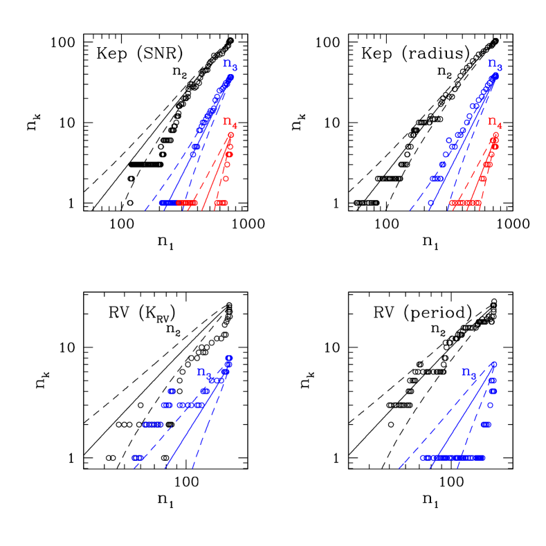
Figure 1: The observable multiplicity function for subsets of the Kepler and radial-velocity planet samples (top and bottom panels, respectively). The catalog subsets are defined by imposing cuts based on signal-to-noise ratio (SNR), planet radius, orbital period, or velocity semi-amplitude ($K_{\mathrm{RV}}$). Open circles show $n_{2}$, $n_{3}$, $n_{4}$ (numbers of 2, 3, and 4-planet systems) as a function of $n_{1}$. Solid and dashed curves show the predictions of equation (12) and the 1–$\sigma$ errors on the predictions.

Example

To illustrate this procedure, we examine the Kepler catalog of Borucki et al. (2011), trimmed by 20% as described at the start of §4 to produce a more homogeneous set of target stars. This is catalog A. All of the planets in this catalog are detected with a signal/noise ratio (SNR) of at least 7. We construct a sequence of shallower catalogs (catalogs “B”) by gradually increasing the minimum SNR up to values exceeding 100, at which point only a handful of multi-planet systems is left. The relation (12) implies that apart from statistical fluctuations the numbers of multiple-planet systems $n_{k}^{B}$, $k=1,\ldots$, are functions only of $f^{BA}$ and the known $\mathbf{n}^{A}$, which approximates the observable multiplicity function $\overline{\mathbf{n}}^{A}$. Hence by eliminating $f^{BA}$ in favor of $n_{1}^{B}$, the number of $k$-planet systems in any survey B can be predicted as a function of the number of one-planet systems in that survey. These predictions for $k=2,3,4$ are shown in the upper left panel of Figure 1 as solid lines, along with the 1–$\sigma$ confidence bands (dashed lines). The actual numbers of multi-planet systems after SNR cuts on the Kepler data are shown as open circles. Within the statistical errors the predictions agree with the data for $k=2$ and 3 and are marginally consistent for $k=4$: using a Kolmogorov–Smirnov (KS) test, the $p$-value (probability of observing deviations at least as extreme as those seen, given the null hypothesis) is 0.28, 0.27, and 0.06 respectively.

The upper right panel of Figure 1 shows a similar comparison for a sequence of catalogs based on cuts at increasing planet radius, rather than SNR. The results are consistent with the separable model to within the statistical errors ($p$-values of 0.72, 0.19, and 0.66 for $k=2,3,4$).

The lower panels of Figure 1 show similar results for radial-velocity surveys. The “A” catalog consists of 240 FGK dwarf stars hosting one or more planets (see eq. 46 for more detail), and the cuts are based on $K_{\mathrm{RV}}$ (semi-amplitude of the radial-velocity curve) on the left and orbital period on the right. The predictions are marginally consistent with the null hypothesis ($p$-values between 0.03 and 0.10) except for $n_{2}$ as a function of the cut in $K_{\mathrm{RV}}$, for which the null hypothesis is excluded.

These results confirm that in many cases the separability approximation and equation (12) provide useful tools for removing survey selection effects and converting the observable multiplicity function between surveys.

3 Geometric selection effects in transiting systems

Throughout this paper we shall assume that tranets are in circular orbits. Moorhead et al. (2011) estimate that the mean eccentricity of planets discovered in the Kepler survey is only 0.1–0.25, so this assumption should not cause significant errors. We shall also assume that a transit occurs when the line of sight to the center of the planet intersects the stellar disk. This assumption should be approximately correct so long as the planetary radius is much smaller than the stellar radius (the median ratio of planetary radius to stellar radius in the Kepler survey is only 0.026).

Let $R_{\star}$ be the radius of the star, $a$ the semi-major axis of a planet in a circular orbit, and $\epsilon\equiv R_{\star}/a$. Consider a system containing $n$ planets with semi-major axes specified by $\epsilon_{1},\ldots,\epsilon_{n}$. Let $g_{mn}(\epsilon_{1},\ldots,\epsilon_{n})$ be the probability that a randomly oriented observer will detect $m$ tranets in this system.

One planet

First consider the case $n=1$. We define three unit vectors: $\hat{\bf o}$ points towards the observer, $\hat{\bf n}$ is normal to the planetary orbit, and $\hat{\bf z}$ is normal to the reference plane from which inclinations $i$ are measured. Thus $\hat{\bf z}\cdot\hat{\bf n}=\cos i$ and $\hat{\bf o}\cdot\hat{\bf n}=\cos\gamma$. If the planet’s size is negligible, it transits if and only if $|\hat{\bf o}\cdot\hat{\bf n}|<\epsilon$ or $|\cos\gamma|<\epsilon$ so

$$g_{11}(\epsilon)=1-g_{01}(\epsilon)=\frac{\int_{|\cos\gamma|<\epsilon}\sin\gamma\,d\gamma}{\int\sin\gamma\,d\gamma}=\epsilon.$$ (13)

Two planets

Let $h(w)=1$ if $|w|<1$ and zero otherwise. Then transits occur if and only if $h(\epsilon^{-1}\cos\gamma)$ is unity and we may write

$$h(\epsilon^{-1}\cos\gamma)=\sum_{\ell=0}^{\infty}b_{\ell}(\epsilon)P_{\ell}(\cos\gamma)$$ (14)

where $P_{\ell}$ is a Legendre polynomial. From the properties of these functions we have

$$b_{\ell}(\epsilon)=\left\{\begin{array}[]{ll}\epsilon,&\ell=0,\\ P_{\ell+1}(\epsilon)-P_{\ell-1}(\epsilon),&\ell\hbox{ even, }\ell>0\\ 0,&\ell\hbox{ odd.}\end{array}\right.$$ (15)

Now let $(\theta,\phi)$ be the polar coordinates for $\hat{\bf o}$ relative to the polar axis $\hat{\bf z}$, and $(\Omega-\textstyle{\frac{1}{2}}\pi,i)$ the polar coordinates for $\hat{\bf n}$. Then

$$h(\epsilon^{-1}\cos\gamma)=4\pi\sum_{\ell=0}^{\infty}\frac{b_{\ell}(\epsilon)}{2\ell+1}\sum_{m=-\ell}^{\ell}Y_{\ell m}^{\ast}(\theta,\phi)Y_{\ell m}(i,\Omega-\textstyle{\frac{1}{2}}\pi).$$ (16)

Let the probability distribution of planetary inclinations be $q(i|\mbox{\boldmath$\kappa$})di$, where $\kappa$ is a set of free parameters describing the inclination distribution, which we may vary to fit the observations. Then the probability of a transit of a single planet, given the observer orientation $x\equiv\cos\theta$, is

$$u(x|\epsilon,\mbox{\boldmath$\kappa$})=\int\frac{di\,d\Omega}{2\pi}q(i|\mbox{\boldmath$\kappa$})h(\epsilon^{-1}\cos\gamma)= 4\pi\sum_{\ell=0}^{\infty}\frac{b_{\ell}(\epsilon)}{2\ell+1}\int di\,q(i|\mbox{\boldmath$\kappa$})Y_{\ell 0}^{\ast}(\theta,0)Y_{\ell 0}(i,0)$$

$$= \sum_{\ell=0}^{\infty}Q_{\ell}(\mbox{\boldmath$\kappa$})\,b_{\ell}(\epsilon)P_{\ell}(x).$$ (17)

where

$$Q_{\ell}(\mbox{\boldmath$\kappa$})\equiv\int_{0}^{\pi}di\,q(i|\mbox{\boldmath$\kappa$})P_{\ell}(\cos i),\quad Q_{0}=1.$$ (18)

If a system contains two planets, the probability that both transit for a random orientation of the observer is

$$g_{22}(\epsilon_{1},\epsilon_{2},\mbox{\boldmath$\kappa$})= \textstyle{\frac{1}{2}}\int_{-1}^{1}dx\,u(x|\epsilon_{1},\mbox{\boldmath$\kappa$})u(x|\epsilon_{2},\mbox{\boldmath$\kappa$})$$

$$= \textstyle{\frac{1}{2}}\sum_{\ell,n=0}^{\infty}b_{\ell}(\epsilon_{1})b_{n}(\epsilon_{2})Q_{\ell}(\mbox{\boldmath$\kappa$})Q_{n}(\mbox{\boldmath$\kappa$})\int_{-1}^{1}dx\,P_{\ell}(x)P_{n}(x)$$

$$= \sum_{\ell=0}^{\infty}\frac{Q_{\ell}^{2}(\mbox{\boldmath$\kappa$})}{2\ell+1}b_{\ell}(\epsilon_{1})b_{\ell}(\epsilon_{2}).$$ (19)

Moreover the probability that one and only one of the two planets transits is

$$g_{12}(\epsilon_{1},\epsilon_{2},\kappa)= \textstyle{\frac{1}{2}}\int_{-1}^{1}dx\,\left\{u(x|\epsilon_{1},\mbox{\boldmath$\kappa$})[1-u(x|\epsilon_{2},\mbox{\boldmath$\kappa$})]+[1-u(x|\epsilon_{1},\mbox{\boldmath$\kappa$})]u(x|\epsilon_{2},\mbox{\boldmath$\kappa$})]\right\}$$

$$= g_{11}(\epsilon_{1},\mbox{\boldmath$\kappa$})+g_{11}(\epsilon_{2},\mbox{\boldmath$\kappa$})-2g_{22}(\epsilon_{1},\epsilon_{2},\mbox{\boldmath$\kappa$})$$ (20)

and the probability that no planets transit is

$$g_{02}(\epsilon_{1},\epsilon_{2},\mbox{\boldmath$\kappa$})= 1-g_{12}(\epsilon_{1},\epsilon_{2},\mbox{\boldmath$\kappa$})-g_{22}(\epsilon_{1},\epsilon_{2},\mbox{\boldmath$\kappa$})$$

$$= 1-g_{11}(\epsilon_{1},\mbox{\boldmath$\kappa$})-g_{11}(\epsilon_{2},\mbox{\boldmath$\kappa$})+g_{22}(\epsilon_{1},\epsilon_{2},\mbox{\boldmath$\kappa$}).$$ (21)

For example, if the planets are distributed isotropically then $q(i)di=\textstyle{\frac{1}{2}}\sin i\,di$, $Q_{\ell}=\delta_{\ell 0}$ and $g_{22}(\epsilon_{1},\epsilon_{2})=\epsilon_{1}\epsilon_{2}$. If the planets have zero inclination, it can be shown that

$$g_{22}(\epsilon_{1},\epsilon_{2})=\sum_{\ell=0}^{\infty}\frac{b_{\ell}(\epsilon_{1})b_{\ell}(\epsilon_{2})}{2\ell+1}=\hbox{min\,}(\epsilon_{1},\epsilon_{2}),$$ (22)

although this result is derived more easily in other ways.

Three or more planets

These results can be extended to any number of planets:

$$g_{mn}(\epsilon_{1},\ldots,\epsilon_{n},\mbox{\boldmath$\kappa$})=\textstyle{\frac{1}{2}}\int_{-1}^{1}dx\,\sum_{P_{n}}\prod_{i=1}^{m}u(x|\epsilon_{p_{i}},\mbox{\boldmath$\kappa$})\prod_{j=m+1}^{n}[1-u(x|\epsilon_{p_{j}},\mbox{\boldmath$\kappa$})],$$ (23)

where $P_{n}$ is the set of all permutations $(p_{1},\ldots,p_{n})$ of the numbers $1,\ldots,n$, and $m\leq n$. For example,

$$g_{23}(\epsilon_{1},\epsilon_{2},\epsilon_{3},\mbox{\boldmath$\kappa$}) =g_{22}(\epsilon_{1},\epsilon_{2},\mbox{\boldmath$\kappa$})+g_{22}(\epsilon_{2},\epsilon_{3},\mbox{\boldmath$\kappa$})+g_{22}(\epsilon_{3},\epsilon_{1},\mbox{\boldmath$\kappa$})-3g_{33}(\epsilon_{1},\epsilon_{2},\epsilon_{3},\mbox{\boldmath$\kappa$})$$

$$g_{13}(\epsilon_{1},\epsilon_{2},\epsilon_{3},\mbox{\boldmath$\kappa$}) =g_{11}(\epsilon_{1},\mbox{\boldmath$\kappa$})+g_{11}(\epsilon_{2},\mbox{\boldmath$\kappa$})+g_{11}(\epsilon_{3},\mbox{\boldmath$\kappa$})-2g_{22}(\epsilon_{1},\epsilon_{2},\mbox{\boldmath$\kappa$})-2g_{22}(\epsilon_{2},\epsilon_{3},\mbox{\boldmath$\kappa$})$$

$$\quad\quad\quad-2g_{22}(\epsilon_{3},\epsilon_{1},\mbox{\boldmath$\kappa$})+3g_{33}(\epsilon_{1},\epsilon_{2},\epsilon_{3},\mbox{\boldmath$\kappa$}).$$ (24)

The geometric selection matrix $G_{mn}$ (eq. 1) is simply $\langle g_{mn}(R_{\star}/a_{1},R_{\star}/a_{2},\ldots,R_{\star}/a_{l},\mbox{\boldmath$\kappa$})\rangle$, the average of the geometric selection factor over the joint distribution of stellar radius $R_{\star}$ and planetary semi-major axis $a$ for the survey. To evaluate $G_{mn}(\mbox{\boldmath$\kappa$})$ we use the separability assumption (4) with respect to $\epsilon=R_{\star}/a$. Thus

$$G_{mn}(\mbox{\boldmath$\kappa$})=\int g_{mn}(\epsilon_{1},\ldots,\epsilon_{n},\mbox{\boldmath$\kappa$})\prod_{k=1}^{n}f(\epsilon_{k})d\log\epsilon_{k},$$ (25)

where $f(\epsilon)d\log\epsilon$ represents the probability distribution of $\epsilon$ as modified by the survey selection effects.

With this parametrization and equations (17) and (23) it is straightforward to show that $G_{mn}(\mbox{\boldmath$\kappa$})$ is given by the binomial distribution,

$$G_{mn}(\mbox{\boldmath$\kappa$})=\frac{n!}{2m!(n-m)!}\int_{-1}^{1}dx\,U^{m}(x|\mbox{\boldmath$\kappa$})[1-U(x|\mbox{\boldmath$\kappa$})]^{n-m}=\textstyle{\frac{1}{2}}\int_{-1}^{1}dx\,S_{mn}[U(x|\mbox{\boldmath$\kappa$})]$$ (26)

where $S_{mn}$ is given by equation (7),

$$U(x|\mbox{\boldmath$\kappa$})\equiv\frac{\int f(\epsilon)u(x|\epsilon,\mbox{\boldmath$\kappa$})\,d\log\epsilon}{\int f(\epsilon)\,d\log\epsilon}=\sum_{\ell=0}^{\infty}Q_{\ell}(\mbox{\boldmath$\kappa$})B_{\ell}P_{\ell}(x),$$ (27)

and

$$B_{\ell}\equiv\int f(\epsilon)b_{\ell}(\epsilon)\,d\log\epsilon\quad\mbox{with}\quad\int f(\epsilon)\,d\log\epsilon=1.$$ (28)

Since $B_{\ell}$ does not depend on the unknown parameters $\kappa$ of the inclination distribution it can be evaluated once and for all at the start of any optimization procedure. It is straightforward to show that the relations (2) are satisfied by these formulae, and that the matrices $\mathbf{G}$ and $\mathbf{S}$ commute. In numerical work we typically truncate infinite series such as (27) at $\ell=\ell_{\rm max}=50$, but for very thin disks it may be necessary to include terms of higher $\ell$.

We pointed out in equation (10) that most survey selection effects preserve the separability assumption. This result does not generally hold for geometric selection effects. To illustrate this, consider the simple case of a population of stars containing two planets, with zero relative inclination. Write the probability distribution of $\epsilon=R_{\star}/a$ of two-planet systems as $f(\epsilon_{1})f(\epsilon_{2})d\log\epsilon_{1}d\log\epsilon_{2}$ (after survey selection effects but before geometric selection effects). Then using equation (22) it is evident that the probability distribution of two-tranet systems is

$$dp_{2}(\epsilon_{1},\epsilon_{2})=f(\epsilon_{1})f(\epsilon_{2})\hbox{min\,}(\epsilon_{1},\epsilon_{2})\,d\log\epsilon_{1}\,d\log\epsilon_{2},$$ (29)

which is not separable. Only for isotropic distributions do geometric selection effects preserve separability.

3.1 The inclination distribution

In this paper we model the probability distribution of the inclinations $dp=q(i|\kappa)di$ as a Fisher distribution,

$$q(i|\kappa)=\frac{\kappa}{2\sinh\kappa}\exp(\kappa\cos i)\sin i.$$ (30)

The parameter $\kappa$ is related to the mean-square value of $\sin i$ through

$$\langle\sin^{2}i\rangle=\int di\sin^{2}i\,q(i|\kappa)=2\frac{\coth\kappa}{\kappa}-\frac{2}{\kappa^{2}}.$$ (31)

When $\kappa\ll 1$ the Fisher distribution approaches an isotropic distribution, $\lim_{\kappa\to 0}q(i|\kappa)=\frac{1}{2}\sin i$, while for $\kappa\gg 1$ it approaches the Rayleigh distribution, $\lim_{\kappa\to\infty}q(i|\kappa)=(2i/s^{2})\*\exp(-i^{2}/s^{2})$ where $s=(2/\kappa)^{1/2}$ is the rms inclination and $\frac{1}{2}\pi^{1/2}s=0.8862s$ is the mean inclination. The Rayleigh distribution is commonly used to model the inclination distribution of asteroids, Kuiper-belt objects, stars in the Galactic disk (where it is known as the Schwarzschild distribution), etc. As $\kappa\to-\infty$ the Fisher distribution approaches a retrograde Rayleigh distribution.

For the Fisher distribution, equation (18) becomes

$$Q_{\ell}(\kappa)=\sqrt{\frac{\pi\kappa}{2}}\frac{I_{\ell+1/2}(\kappa)}{\sinh\kappa}$$ (32)

where $I$ denotes a modified Bessel function.

3.2 Validity of the separability assumption

There is limited evidence on the accuracy of the separability approximation for multi-planet systems. First consider RV surveys, in which there are no geometric selection effects. The most important survey selection effects depend only on the properties of an individual planet so an RV survey of a separable parent distribution should lead to a separable detected distribution (eq. 10).

Wright et al. (2009) compare 28 multi-planet systems and a much larger number of single-planet systems detected by RV surveys. They find that (i) the eccentricities in multi-planet systems are smaller (mean eccentricity 0.22, compared to 0.30 in single-planet systems); (ii) the logarithmic semi-major axis distribution in multi-planet systems is flatter, without the pileup of hot Jupiters between $0.03\,\textsc{au}$ and $0.07\,\textsc{au}$ and the enhancement outside $1\,\textsc{au}$ that are seen in single-planet systems; (iii) multi-planet systems exhibit an overabundance of planets with minimum mass between 0.01 and 0.2 Jupiter masses. These differences are incompatible with separability and statistically significant ($p<0.03$), but relatively small: they represent maximum differences of only 0.18, 0.17, and 0.26 in the cumulative probability distributions for eccentricity, semi-major axis, and minimum mass. Wright et al. (2009) point out that the last of these differences may also be amplified by an unmodeled survey selection effect—stars hosting planets tend to be observed more frequently, thereby enhancing the chance to discover additional low-mass planets. Most of the plots in the lower panels of Figure 1 are marginally consistent with separability, as discussed at the end of §2.

The evidence on separability from the Kepler survey is more difficult to interpret, because geometric selection effects do not preserve separability (see discussion just before §3.1). Nevertheless, the semi-major axis distributions of single- and multiple-tranet systems in the Kepler survey are indistinguishable according to a KS test ($p$-value 0.20; see also Figure 2), which is consistent with separability. Presumably the pileup of hot Jupiters at small semi-major axes seen in the RV surveys is less prominent in the Kepler sample because the typical planetary mass is much smaller, and the jump outside $1\,\textsc{au}$ is not seen because Kepler is not sensitive to these orbital periods.

Latham et al. (2011) have shown that Kepler systems with multiple tranets are less likely to include a giant planet (larger than Neptune) than systems with a single tranet. We confirm using a KS test that the distributions of radii in the single- and multiple-tranet systems are different (maximum difference in the cumulative probability distribution of 0.20). However, the results at the end of §2 show that the numbers of two-, three-, and four-tranet systems as a function of the radius cutoff appear to be consistent with separability. Evidently equations such as (11) that we use to compare the observable multiplicity function between surveys are less sensitive to deviations from separability than statistical tests designed specifically for this purpose.

These comparisons suggest that deviations from separability, though present in both the RV and Kepler planet samples, are not large enough to compromise our method and results. However, further exploration of both the magnitude and the effects of these deviations is needed.

4 Estimating the inclination distribution and the multiplicity function from the Kepler survey

4.1 Properties of the survey

The Kepler survey has a complex set of survey selection effects, which we do not attempt to model. The constraints on the multiplicity function that we derive therefore apply to the population of planets in radius, semi-major axis, etc. that Kepler detects, whatever that population may be (for a discussion of selection effects and completeness in the Kepler catalog see Howard et al. 2011 and Youdin 2011). If we denote the multiplicity function of this population by $\mathbf{N}$ and the observable multiplicity function of the Kepler survey by $\overline{\mathbf{n}}$ then equation (1) becomes

$$\overline{\mathbf{n}}=\mathbf{G}\cdot\mathbf{N}.$$ (33)

The validity of this equation requires only the plausible assumption that the probability that Kepler will detect a given transiting planet around a given star is independent of whether it detects other transits around the same star.

To produce a more homogeneous sample, we trim the catalog of Borucki et al. (2011) to include only stars with effective temperatures between 4000 and 6500 K and surface gravity $\log g>4.0$ (roughly equivalent to FGK dwarfs), and to Kepler magnitudes between 9.0 and 16.0; this trimming leaves 124,613 stars from the original sample of 153,196. We also restrict the catalog to planets with orbital period less than 200 d and radius less than 2 Jupiter radii; this leaves 1092 planets from the original sample of 1235. The numbers of stars with $0,1,2,\ldots$ tranets are

$$\begin{array}[]{cccc}n_{0}=1.237\times 10^{5},&n_{1}=737,&n_{2}=104,&n_{3}=37,\\ n_{4}=7,&n_{5}=1,&n_{6}=1,&n_{k}=0\hbox{ for }k>6.\end{array}$$ (34)

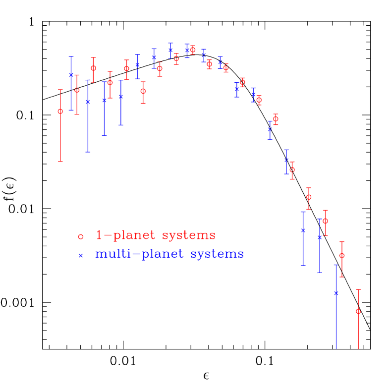
Figure 2: The probability distribution of $\epsilon=R_{\star}/a$, the ratio of stellar radius to planetary semi-major axis, for tranets detected by Kepler. The differential probability distribution is $dp=f(\epsilon)\,d\log\epsilon$. The data points for single- and multi-tranet systems are shown separately. The solid line shows the analytic fitting formula (35).

We need to determine the function $f(\epsilon)$, where $f(\epsilon)\,d\log\epsilon$ is the fraction of planets in the range $d\log\epsilon$ given the intrinsic distribution of planets and the survey selection effects for Kepler. As usual $\epsilon=R_{\star}/a$ is the ratio of stellar radius to planetary semi-major axis; the stellar radius is determined from the host-star mass and surface gravity and the semi-major axis is determined from the host-star mass and the planetary orbital period. Figure 2 shows data points for $f(\epsilon)$ from single-tranet systems (red points) and from planets in multi-tranet systems (blue points). The data points have been constructed by adding a contribution of $\epsilon^{-1}$ (to account for geometric selection effects) from each tranet to the corresponding bin, then normalizing so that the integral over $\log\epsilon$ is unity. The distributions for single-tranet and multi-tranet systems are quite similar, and can be adequately fit by the parametrization

$$f(\epsilon)=0.656\frac{(\epsilon/\epsilon_{0})^{0.5}}{1+(\epsilon/\epsilon_{0})^{3.6}},\quad\epsilon_{0}=0.055,\quad\mbox{for }\epsilon>0.004$$ (35)

and zero for $\epsilon<0.004$. The sharp decline for $\epsilon\gtrsim 0.1$ is due to an absence of planets with semi-major axis $\lesssim 0.04\,\textsc{au}$ (Borucki et al., 2011), while the cutoff at $\epsilon\lesssim 0.004$ is due to the limited timespan of the Kepler data.

4.2 Statistical method

The probability that the survey actually detects $\{n_{0},n_{1},\ldots,n_{K}\}$ stars having $0,1,\ldots,K$ planets is

$$P(\mathbf{n}|\mathbf{N},\mbox{\boldmath$\kappa$})=\prod_{k=0}^{K}\frac{\overline{n}_{k}^{n_{k}}\exp(-\overline{n}_{k})}{n_{k}!}$$ (36)

where $\mathbf{n}=(n_{0},n_{1},\ldots,n_{K})$ and $\overline{n}_{k}$ is related to $\mathbf{N}$ by equation (33).

Estimating the multiplicity function $\mathbf{N}$ and the inclination distribution parameters $\kappa$ from $\mathbf{n}$ is a straightforward but challenging problem in statistics and optimization. This problem can be attacked with a variety of methods (linear programming, minimum $\chi^{2}$, maximum likelihood, Bayesian analysis using a Markov chain Monte Carlo algorithm, etc.), and we have experimented with most of these. In this paper we have usually chosen maximum likelihood, as a reasonable compromise between generality, computation time, and clarity of interpretation.

The log of the likelihood of a given observational result $\mathbf{n}$ is

$$\log P(\mathbf{n}|\mathbf{N},\mbox{\boldmath$\kappa$})=\sum_{k=0}^{K}n_{k}\log\left[\sum_{l=k}^{K}G_{kl}(\mbox{\boldmath$\kappa$})N_{l}\right]-\sum_{k=0}^{K}\sum_{l=k}^{K}G_{kl}(\mbox{\boldmath$\kappa$})N_{l}-\sum_{k=0}^{K}\log n_{k}!.$$ (37)

Note that the second term on the right can be simplified to $\sum_{l}N_{l}$ using equation (3). We then maximize $\log P$ with respect to $\mathbf{N}$ and $\kappa$, subject to the constraint $N_{k}\geq 0$, $k=0,\ldots,K$.

4.3 Results

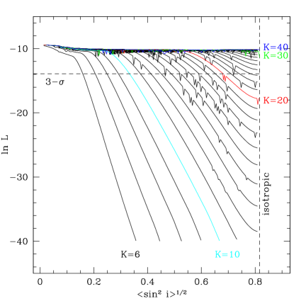
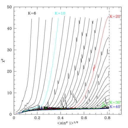
Figure 3: (top) The maximum likelihood of solutions for the multiplicity function of the Kepler survey, as a function of rms inclination and maximum number $K$ of planets per system. Solid lines connect solutions with a given $K$, $6\leq K\leq 40$; lines for $K=10,20,30,40$ are colored cyan, red, green, and blue for emphasis. The vertical dashed line denotes isotropic planetary systems. The horizontal dashed line marks systems that are 3-$\sigma$ ($\Delta\ln L=4.5$) lower in likelihood than razor-thin solutions, $\langle\sin^{2}i\rangle=0$. (bottom) Plots of $\chi^{2}$ (eq. 39) for the maximum-likelihood models shown above. We estimate that models with $\chi^{2}\lesssim 5$ are good fits to the data.

The top panel of Figure 3 shows the maximum likelihood as a function of the rms inclination and the maximum number of planets per system, $K$, for $6\leq K\leq 40$. The minimum allowed value is $K=6$ since Kepler has found one system with six tranets. The maximum-likelihood models with a given $K$ are connected to form solid lines, and the families with $K=10$, 20, 30, and 40 are colored for emphasis. There are occasional small dips in the lines when the optimization algorithm (a quasi-Newton algorithm from NAG) converged on a local rather than global maximum. The figure shows that:

(i) The highest likelihood is for razor-thin systems, with near zero rms inclination. However, the preference for zero rms inclination has only marginal statistical significance: systems exist at all rms inclinations—even isotropic systems—with log likelihood only 0.73 smaller than the razor-thin solutions.

(ii) Systems with large rms inclinations are only consistent with the data if a fraction of them contain a large number of planets. At the 3-$\sigma$ level (log likelihood smaller than the maximum by 4.5, marked by a horizontal dashed line on the figure), the maximum rms inclination is related to the maximum number of planets by

$$\langle\sin^{2}i\rangle^{1/2}\leq\left\{\begin{array}[]{ll}0.15+0.037(K-6),&K<24\\ (\frac{2}{3})^{1/2}\mbox{ (isotropic)},&K\geq 24.\end{array}\right.$$ (38)

It is possible, of course, that even the maximum-likelihood model does not fit the data well. To explore this possibility, we have calculated the standard Pearson $\chi^{2}$ statistic,

$$\chi^{2}=\sum_{k=0}^{K}\frac{(n_{k}-\overline{n}_{k})^{2}}{\overline{n}_{k}}=\sum_{k=0}^{K}\frac{(n_{k}-\sum_{l}G_{kl}N_{l})^{2}}{\sum_{l}G_{kl}N_{l}}.$$ (39)

The distribution of the $\chi^{2}$ statistic is not straightforward to interpret, since $\overline{n}_{k}\lesssim 1$ for many $k$ and since the number of degrees of freedom is not well-defined. Nevertheless it is probably reasonable to expect that there is a good fit to the data if $\chi^{2}\lesssim 5$. The values of $\chi^{2}$ for the maximum-likelihood solutions in the top panel of Figure 3 are shown in the bottom panel of that figure. There are satisfactory models with all rms inclinations, but as before such models require that some systems contain many planets if the rms inclination is large.

It is instructive to examine the isotropic solution with $K=30$ in more detail (the behavior of the isotropic solutions with $K>30$ is qualitatively similar). The fraction of stars with $k$-planet systems is

$$\frac{N_{k}}{\sum_{l=0}^{K}N_{l}}=\left\{\begin{array}[]{ll}0.944&k=0,\\ 0.0065&k=1,\\ 0&k=2,\\ 0.0452&k=3,\\ 0&k=4,\ldots,29,\\ 0.0043&k=30.\end{array}\right.$$ (40)

Thus, in this solution, about half of the planets are contained in three-planet systems, and the other half in a small population ($<0.5\%$) of stars with many-planet systems. This multiplicity function and inclination distribution are neither unique nor particularly plausible but they are consistent with the Kepler data.

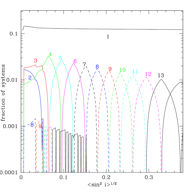
Figure 4: The fraction of stars in the Kepler sample containing $k$-planet systems, as a function of the rms value of $\sin i$. The curves are labeled by $k$ for $k\leq 13$ and curves with $7\leq k\leq 12$ are dashed. These curves were obtained by linear programming, using the constraint that $\overline{n}_{k}$ must lie within the 90% confidence interval determined through equation (36). The cost function minimized the total number of planets but the result is insensitive to this choice.

Figure 4 shows the fraction of stars in the Kepler sample with $0,1,2,3,\dots$-planet systems, as a function of the assumed rms inclination. The results are for $K=30$ but are qualitatively similar for larger values of $K$. Our initial attempts to construct this figure were unsuccessful, because the appearance of the figure is very sensitive to cases when the optimization algorithm settles on a local maximum of the likelihood. To avoid this difficulty, we re-cast the optimization as a problem in linear programming: we demanded that each $\overline{n}_{k}$ should lie within the 90% confidence interval determined by the Poisson distribution (36), and from these solutions we chose the one with the minimum total number of planets $\sum_{k=1}^{K}N_{k}$. This specifies a unique solution, if one exists.

At the smallest inclinations ($\langle\sin^{2}i\rangle^{1/2}<0.05$) the solution contains a mix of 1,2,3,4, and 8 or 9-planet systems. As the rms inclination increases, the mixture becomes strongly dominated by 1-planet and $n_{i}$-planet systems where $n_{i}$ varies monotonically with the rms inclination—for example, $n_{i}=12$ when $\langle\sin^{2}i\rangle^{1/2}\simeq 0.3$. We caution that these results should not be regarded as a prediction of the Kepler multiplicity function for a given rms inclination.

The need for many-planet systems is straightforward to understand. Consider the extreme case of an isotropic distribution. Then $\kappa=0$ and $q(i|\kappa=0)=\frac{1}{2}\sin i$; thus $Q_{\ell}(\kappa=0)=\delta_{\ell 0}$ from equation (18) and the orthogonality properties of the Legendre polynomials. Thus $U(x|\kappa=0)=B_{0}$ (eq. 27) and using equation (26)

$$G_{mn}(\mbox{\boldmath$\kappa$})=\frac{n!}{m!(n-m)!}B_{0}^{m}(1-B_{0})^{n-m}.$$ (41)

If all systems contain $n$ planets, the ratio of the number of $m$-tranet systems to the number of $(m+1)$-tranet systems is

$$\frac{G_{mn}}{G_{m+1,n}}=\frac{m+1}{n-m}\frac{1-B_{0}}{B_{0}},\quad n\geq m+1.$$ (42)

Using equations (28) and (35) we find that $B_{0}=0.0321$ for the Kepler survey. From equation (34) we find $n_{1}/n_{2}=7.1\pm 0.7$. For comparison the ratio $G_{1n}/G_{2n}$ is less than $7.1+0.7=7.8$ only for $n\geq 9$; thus any population dominated by systems with less than 9 planets will overproduce 1-tranet systems relative to 2-tranet systems. Similarly, for the Kepler survey $n_{2}/n_{3}=2.8\pm 0.5$, and $G_{2n}/G_{3n}>2.8+0.5=3.3$ unless $n\geq 30$.

The average number of planets per star from these solutions is shown in Figure 5. This result is insensitive to the rms inclination and the maximum number of planets per star ($K$), since it is given simply by the ratio of the total number of planets to the number of target stars, divided by the probability that a single randomly oriented planet will transit (Youdin, 2011). Mathematically,

$$\langle\mbox{number of planets per star}\rangle=\frac{\sum_{k=1}^{K}kn_{k}}{B_{0}\sum_{k=0}^{K}n_{k}}=0.274.$$ (43)

The large open circles in Figure 5 show the probability that a system with one, two, or three tranets has additional planets. Typically the fraction of one-tranet systems with additional planets is 0.2–0.5, without a strong dependence on rms inclination. For two or three tranets the probability that there are additional unseen planets is substantially higher. The additional planets may be detectable by transit timing variations (Ford et al., 2011).

Figure 5: The horizontal blue line, composed of $\sim 7000$ points from individual maximum-likelihood models, shows the average number of planets per star in the Kepler sample, as a function of the rms inclination and the maximum number of planets per star, $11\leq K\leq 40$. The large open circles show the probability that a system exhibiting one, two, or three tranets has additional planets.

5 Combining Kepler and radial-velocity surveys

As described in the Introduction, a comparison of the observable multiplicity functions of planetary systems detected by radial velocities and by transits can offer a powerful probe of the inclination distribution. The principal obstacle to making this comparison is that the masses and orbital periods of the planets detected through these two observational techniques are quite different, as illustrated in Figure 6, and the multiplicity functions in these two regions of parameter space are likely to be different. In this section we use the separability approximation and the methods of §2 to overcome this obstacle.

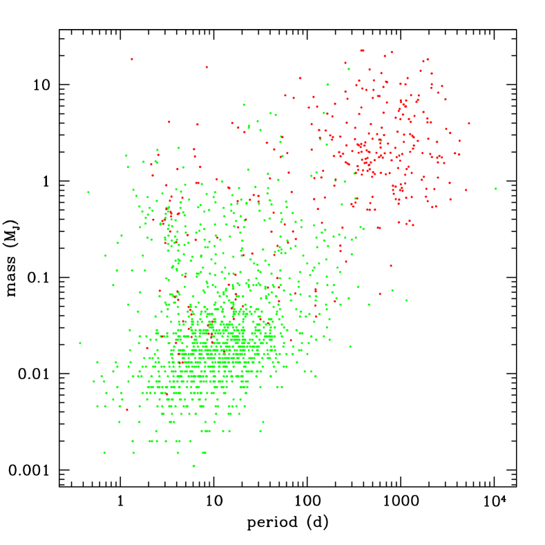
Figure 6: The orbital periods and masses of the planets detected by Kepler (green) and by ground-based radial-velocity surveys (red). Orbital periods are in days and masses are in Jupiter masses. Masses $M$ for transiting planets are computed from radii $R$ using $M=(R/R_{\oplus})^{2.06}M_{\oplus}$ (Lissauer et al., 2011b, for a more accurate relation see eq. 47) and masses for radial-velocity planets are minimum masses $M\sin\gamma$.

Suppose that we wish to combine the Kepler survey with a radial-velocity (RV) survey (or a set of such surveys). The surveys yield $n_{k}^{\mathrm{Kep}}$ and $n_{k}^{\mathrm{RV}}$ systems containing $k$ planets. We assume that both surveys have similar target star populations (we cull the list of target stars in both cases to include only FGK dwarfs), with multiplicity function $\mathbf{N}$ for Kepler and $c\,\mathbf{N}$ for the RV survey, where $c<1$ is a constant to be determined. Let $\mathbf{S}(W^{\mathrm{Kep}})$ and $\mathbf{S}(W^{\mathrm{RV}})$ be the survey selection functions. We assume that there are no geometric selection effects for the RV surveys (cf. footnote 2). The generalization of equation (36) for the likelihood is

$$P(\mathbf{n}^{\mathrm{Kep}},\mathbf{n}^{\mathrm{RV}}|\mathbf{N},\mbox{\boldmath$\kappa$})=\prod_{k=0}^{K}\frac{(\overline{n}_{k}^{\mathrm{Kep}})^{n_{k}^{\mathrm{Kep}}}\exp(-\overline{n}_{k}^{\mathrm{Kep}})}{n_{k}^{\mathrm{Kep}}!}\prod_{k=1}^{K}\frac{(\overline{n}_{k}^{\mathrm{RV}})^{n_{k}^{\mathrm{RV}}}\exp(-\overline{n}_{k}^{\mathrm{RV}})}{n_{k}^{\mathrm{RV}}!}$$ (44)

where

$$\overline{\mathbf{n}}^{\mathrm{Kep}}=\mathbf{G}(\mbox{\boldmath$\kappa$})\mathbf{S}(W^{\mathrm{Kep}})\mathbf{N},\quad\overline{\mathbf{n}}^{\mathrm{RV}}=c\,\mathbf{S}(W^{\mathrm{RV}}).$$ (45)

Notice that the second product in equation (44) starts at $k=1$ since it is difficult to determine accurately how many stars have been unsuccessfully examined for planets by RV methods (see further discussion below). We then maximize the likelihood (44) over $N_{0},N_{1},\ldots,N_{K}$, $W^{\mathrm{Kep}}$, $W^{\mathrm{RV}}$, and $c$ (as shown in §2, the likelihood actually depends only on the ratio $W^{\mathrm{RV}}/W^{\mathrm{Kep}}$).

We determine the observable multiplicity function for RV planets using all planets with FGK dwarf host stars in the exoplanets.org database (Wright et al., 2011) as of August 2010,

$$n_{1}^{\mathrm{RV}}=162,\quad n_{2}^{\mathrm{RV}}=24,\quad n_{3}^{\mathrm{RV}}=7,\quad n_{4}^{\mathrm{RV}}=1,\quad n_{5}^{\mathrm{RV}}=1,\quad n_{k}^{\mathrm{RV}}=0\hbox{ for }k>5,$$ (46)

for a total of 240 planets. The observable multiplicity function for Kepler planets is given in equation (34). Figure 7 shows the maximum likelihood as a function of the rms inclination and the maximum number of planets per system, $K$ (top), as well as $\chi^{2}$ for these models (bottom). The plots are noisier than Figure 3, presumably because the optimization algorithm was less successful at finding the global maximum likelihood, but otherwise look similar. In particular, systems with large rms inclinations are consistent with the data if and only if they contain a large number of planets. Evidently adding data from RV surveys has not significantly tightened the constraints on the inclination distribution.

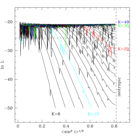
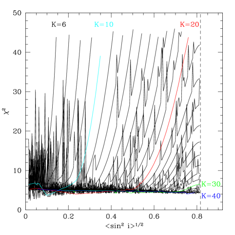
Figure 7: As in Figure 3, except the data include both the Kepler transit survey and radial-velocity surveys.

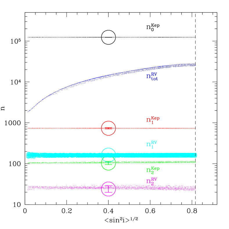
Figure 8: The expected numbers of 0,1,2,3 tranet systems from the Kepler survey and of 1,2,3 planet systems from RV surveys, as predicted by our models. The observed numbers are shown as error bars surrounded by circles. Also shown is the total number of targets in the RV surveys as predicted by our models (blue points).

We now show that adding information on the total number of target stars in the RV surveys does allow the inclination distribution to be determined. Figure 8 shows the expected numbers $\overline{n}_{k}^{\mathrm{Kep}}$ and $\overline{n}_{k}^{\mathrm{RV}}$ of $k$-tranet systems from the Kepler survey and $k$-planet systems from the RV surveys, as determined from the maximum-likelihood solutions described above. Each point corresponds to a given maximum number of planets ($6\leq K\leq 40$) and rms inclination, and only solutions within 3–$\sigma$ of the global maximum likelihood are shown. The points with error bars (surrounded by circles for greater visibility) correspond to the observed numbers $n_{k}^{\mathrm{Kep}}$ and $n_{k}^{\mathrm{RV}}$ from equations (34) and (46). Most of the expected values lie within the error bars of the corresponding observed value; this is no more than a confirmation that our optimization code is performing properly. The blue points show the total number of stars in the RV survey, $\overline{n}_{\mathrm{tot}}^{\mathrm{RV}}=\sum_{k=0}^{K}\overline{n}_{k}^{\mathrm{RV}}$, as determined by the optimization code. The plot shows that $\overline{n}_{\mathrm{tot}}^{\mathrm{RV}}$ is tightly correlated with the rms inclination, so an accurate characterization of the total number of RV target stars would enable the determination of the rms inclination.

This task is challenging given the heterogeneous surveys that have produced the RV planets known at the present time. We have used two distinct approaches, which we now describe.

(i) Cumming et al. (2008) carry out a careful examination of selection effects in the Keck Planet Search, and derive the percentage of F, G, and K stars with a planet in various ranges of orbital period and mass. The sample of RV planets used in our analysis (eq. 46) is not corrected for selection effects, but for sufficiently massive planets and sufficiently short orbital periods it should be complete. For example, for planets more massive than Jupiter, $M\sin\gamma>M_{\mathrm{J}}$, with orbital periods less than one year, $P<1\mbox{ yr}$, the velocity semi-amplitude $K_{\mathrm{RV}}>30\,\mbox{m s}^{-1}$, large enough to be detectable in most surveys. In this mass and period range our sample contains 46 planet-hosting stars and Cumming et al. (2008) estimate that the fraction of stars with planets is $0.019\pm 0.007$, which implies $n_{\mathrm{tot}}^{\mathrm{RV}}=2400\pm 900$. Altering the period range to $P<100\mbox{ d}$ gives $n_{\mathrm{tot}}^{\mathrm{RV}}=2500\pm 1200$ (based on 21 host stars); altering the mass cutoff to $M\sin\gamma>0.5M_{\mathrm{J}}$ gives $n_{\mathrm{tot}}^{\mathrm{RV}}=1900\pm 500$ (based on 63 host stars). This last estimate of $n_{\mathrm{tot}}^{\mathrm{RV}}$ is probably low because the surveys we have used are not all complete at this level.

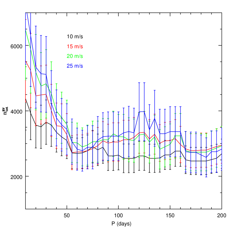
Figure 9: The estimated number of host stars in RV surveys, as determined by comparison with the Kepler survey. The curves and associated error bars show the number of RV host stars as estimated by comparing the number of RV and Kepler planets with period less than $P$ and mass exceeding that required to induce a given velocity semi-amplitude $K_{\mathrm{RV}}$ at period $P$. The observed number of Kepler planets is multiplied by $g_{11}^{-1}$ (eq. 13) to correct for geometric selection effects, and the conversion between radius and mass is given by equation (47). Results are shown for four semi-amplitudes, $K_{\mathrm{RV}}=25,20,15,10\mbox{\,m s}^{-1}$; the plot at the smallest semi-amplitude is low because the RV surveys are incomplete at this level.

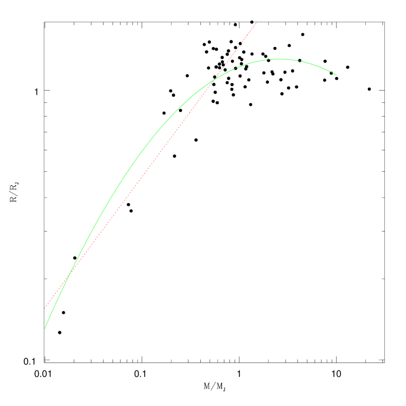
Figure 10: The masses and radii of confirmed transiting exoplanets. The green solid line is the log-quadratic fit in equation (47). The red dashed line is the log-linear fit $\log(M/M_{\oplus})=2.06\log(R/R_{\oplus})$ from Lissauer et al. (2011b).

(ii) We may estimate $n_{\mathrm{tot}}^{\mathrm{RV}}$ using the tranet frequency derived from the Kepler mission. Once again, we restrict the Kepler sample to host stars that are F, G, and K dwarfs (4000 K$<T_{\mathrm{eff}}<$ 6500 K and $\log g>4$). We then carry out the following steps for a given orbital period $P$ and velocity semi-amplitude $K_{\mathrm{RV}}$: (i) compute the corresponding mass $M(P,K_{\mathrm{RV}})=M_{J}(K_{\mathrm{RV}}/30\mbox{\,m s}^{-1})(1\mbox{\,yr}/P)^{1/3}$ assuming a circular orbit and a solar-mass host star; (ii) find the number $n^{\mathrm{RV}}(P,K_{\mathrm{RV}})$ of RV planets with period less than $P$ and mass greater than $M(P,K_{\mathrm{RV}})$; (iii) find all Kepler tranets with mass greater than $M(P,K_{\mathrm{RV}})$ and period less than $P$, using an empirical mass-radius relation found by fitting mass and radius measurements from transiting planets in the range 0.1–$10M_{J}$ (see Figure 10) to a log-quadratic relation

$$\log R/R_{J}=0.087+0.141\log M/M_{J}-0.171\left(\log M/M_{J}\right)^{2};$$ (47)

(iv) compute the total number of Kepler planets in this range $n^{\mathrm{Kep}}(P,K_{\mathrm{RV}})$ by counting each tranet as $\epsilon^{-1}$ planets, to correct for geometric selection effects (eq. 13); (v) estimate the total number of RV host stars as $n_{\mathrm{tot}}^{\mathrm{RV}}=n_{\mathrm{tot}}^{\mathrm{Kep}}n^{\mathrm{RV}}(P,K)/n^{\mathrm{Kep}}(P,K)$. The results are shown in Figure 9 for $K_{\mathrm{RV}}=10,15,20,25\,\mbox{m s}^{-1}$. As the majority of RV surveys have reached precisions of $\sim 15\mbox{\,m s}^{-1}$ or better over the last decade, it is reassuring but not surprising that the estimates of $n_{\mathrm{tot}}^{\mathrm{RV}}$ for $K_{\mathrm{RV}}=15,20,25\mbox{\,m s}^{-1}$ are consistent. The rise in $n^{\mathrm{RV}}_{\mathrm{tot}}$ at small periods is likely due to the known discrepancy in hot Jupiter frequency between transit and RV surveys (the frequency of hot Jupiters estimated from transit surveys is factor of $\sim 2$ smaller than that derived from RV surveys, perhaps because the average metallicities are different; see Gould et al. 2006; Howard et al. 2011).

These independent approaches yield $n^{\mathrm{RV}}_{\mathrm{tot}}\simeq 2500\pm 1000$ and $n^{\mathrm{RV}}_{\mathrm{tot}}\simeq 3000\pm 1000$, respectively, which are consistent within the errors. The corresponding inclination ranges from Figure 8 are $0<\langle\sin^{2}i\rangle^{1/2}<0.08$ and $0.02<\langle\sin^{2}i\rangle^{1/2}<0.09$ which correspond to an rms or mean inclination range of 0–$5^{\circ}$ (as shown in §3.1, for a Rayleigh distribution the rms inclination is only larger than the mean inclination by 12%, which is much less than the uncertainty).

The success of the separability assumption in modeling survey selection effects (§2 and Fig. 1) suggests that our results should be insensitive to cuts made on the Kepler planet candidates. To check this, we have repeated the analysis for the Kepler sample examined by Lissauer et al. (2011b), who imposed a period cut $3\mbox{\,d}<P<125\mbox{\,d}$, a radius cut $1.5R_{\oplus}\leq R\leq 6R_{\oplus}$, and a signal/noise cut SNR$\,\geq 16$, which reduced the number of planets to 63% of our sample. We find the mean inclination for this sample to be 0–$4^{\circ}$, not significantly different from the estimate in the preceding paragraph.

Although the range of rms inclinations is tightly constrained by this analysis, the multiplicity function is not. For example, within 1–$\sigma$ of the maximum-likelihood model ($\Delta\log P\leq 0.5$) we have found models that have no 1-planet systems (67% have no planets, 29% have 2 planets, and 4% have 13 planets) and others that have no zero-planet systems (93% have 1 planet, 2% have 6 planets, and 5% have 25 planets).

A by-product of this analysis is the ratio $W^{\mathrm{RV}}/W^{\mathrm{Kep}}$ (eq. 45), which measures the relative sensitivity of the RV and Kepler surveys. This ratio varies smoothly from 0.5 for razor-thin systems to 0.2 for $\langle\sin^{2}i\rangle^{1/2}=0.1$, independent of the maximum number of planets in the model. In other words 20–50% of the Kepler planets could have been detected in RV surveys. If this ratio can be determined independently by fitting models of the period, radius, and mass distributions it will provide a constraint on the rms inclination that does not require estimating the total number of RV target stars.

A weak link in these arguments is the assumption that the population of FGK dwarf stars is the same in the Kepler and RV surveys. One sign that these populations are different is the higher frequency of hot Jupiters found in RV surveys, as mentioned above. However, we note that our two approaches to estimating $n^{\mathrm{RV}}_{\mathrm{tot}}$, one using only RV surveys and one comparing the Kepler and RV surveys, yield similar answers, which suggests that the estimate of the rms inclination that we derive from this answer is insensitive to differences between the host stars of the Kepler and RV surveys.

It is interesting to compare this estimate of the mean inclination to the mean eccentricity for Kepler planets. Restricting our sample to planets with minimum mass between 0.01 and 0.1 Jupiter masses and period $P>10\mbox{\,d}$ (to avoid the effects of tidal circularization), the mean eccentricity of planets discovered in RV surveys is 0.15 (we have also excluded planets with a reported eccentricity of zero, which may include cases in which no eccentricity was fit). These results are roughly consistent with estimates of the mean eccentricity of Kepler planets from transit timing: Moorhead et al. (2011) find that the mean eccentricity is between 0.13 and 0.25 at a $p$-value of 0.05. We have

$$\frac{\langle i\rangle}{\langle e\rangle}=0.35\frac{\langle i\rangle}{3^{\circ}}\frac{0.15}{\langle e\rangle}.$$ (48)

Theoretical studies of eccentricity and inclination growth in planetesimal disks (e.g., Ida et al., 1993) find $\langle i\rangle/\langle e\rangle=0.45$–0.5, somewhat larger than this value. A possible explanation is that the eccentricities may have been systematically overestimated. Zakamska et al. (2011) find that the typical bias due to measurement errors is $\Delta e\sim 0.04$ in RV catalogs, and the bias in this sample is likely to be higher since the SNR is low for low-mass planets. Possibly a similar bias is present in the Kepler measurements of the eccentricity distribution.

The Kepler survey can measure transit timing variations of a minute or less in favorable cases (Ford et al., 2011). These variations can be used to detect and characterize additional planets. Given the rms inclination of 0–0.09 radians that we have derived, roughly 20–30% of the single-tranet Kepler systems are expected to have additional planets (Figure 5), and many of these may be detectable by transit timing variations. Ford et al. (2011) estimate that $\sim 10$–$20\%$ of suitable Kepler tranets show evidence of transit timing variations, and this number is likely to increase as the survey duration grows. Figure 5 also shows that the fraction of two- or three-tranet systems with additional planets is substantially higher, and strongly dependent on the rms inclination. A preliminary analysis by Ford et al. (2011) yields much lower probabilities of 0.1–0.2 for two- and three-tranet systems; such low probabilities would be difficult to reconcile with any of our models, whatever the rms inclination may be.

6 Summary

We have described a methodology for analyzing the multiplicity function—the fraction of host stars containing a given number of planets—in radial-velocity (RV) and transit surveys. Our approach is based on the approximation of separability, that the probability distribution of planetary parameters in an $n$-planet system is the product of identical 1-planet distributions (§1.2). Exoplanet surveys show that separability is not precisely satisfied but the departures from this approximation are small enough that it provides a powerful tool for the study of multi-planet systems. Using this approximation we have shown how to relate the observable multiplicity function in surveys with different sensitivities, so long as they examine populations of potential host stars with similar properties (§2). We have also shown how to derive the multiplicity function from transit surveys (§3) assuming a given form for the inclination distribution (the Fisher distribution, §3.1). Our principal conclusions are:

1. At present, the Kepler data alone (Borucki et al., 2011) are not able to constrain the inclination distribution of multi-planet systems without additional assumptions or data. In particular, models with all rms inclinations—from razor-thin to spherical—are able to reproduce the observable multiplicity function in the Kepler sample. This conclusion differs from Lissauer et al. (2011b), who found that (i) the Kepler data contained an excess of single-tranet systems that could not be fit by any of their models; (ii) models with mean inclinations exceeding $5^{\circ}$ were poor fits to the data. We believe that these conclusions reflect the restricted, though plausible, range of models for the multiplicity function considered by Lissauer et al. (2011b), although their estimated upper limit to the mean inclination is entirely consistent with our conclusions below based on other methods.

2. Systems with large rms inclinations are only consistent with the Kepler data if at least some of them contain a large number of planets. The relation between rms inclination and maximum number of planets is given by equation (38).

3. In our models, the percentage of one-tranet systems with additional planets is 20–30%, and for two- or three-tranet systems this percentage is even higher (Figure 5). These fractions can be probed observationally using transit timing variations.

4. The rms inclination can be constrained by combining estimates of the observable multiplicity function from Kepler and RV surveys, but only after estimating the effective number of stars that have been examined in RV surveys. We have made two estimates, one using Kepler data and one without; these are consistent, and yield $\langle\sin^{2}i\rangle^{1/2}\leq 0.09$, corresponding to mean inclinations in the range 0–5^∘.

5. Although the range of rms inclinations is tightly constrained by this analysis, the multiplicity function is not: the data are well-fit by (presumably) pathological models containing no zero-planet systems, no one-planet systems, etc.

This research was supported in part by NASA grant NNX08AH83G, and has made use of the Exoplanet Orbit Database and the Exoplanet Data Explorer at exoplanets.org. Work by SD was performed under contract with the California Institute of Technology (Caltech) funded by NASA through the Sagan Fellowship Program. We acknowledge helpful conversations with Dan Fabrycky, Debra Fischer, Matt Holman, Boaz Katz, Darin Ragozzine, and Jason Wright.

References

- Abt (2010) Abt, H. A. 2010, PASP, 122, 1015
- Baluev (2011) Baluev, R. V. 2011, arXiv:1105.4696
- Bean & Seifahrt (2009) Bean, J. L., & Seifahrt, A. 2009, A&A, 496, 249
- Black (1997) Black, D. C. 1997, ApJ, 490, L171
- Borucki et al. (2011) Borucki, W. J., et al. 2011, arXiv:1102.0541
- Correia et al. (2010) Correia, A. C. M., et al. 2010, A&A, 511, A21
- Cumming et al. (2008) Cumming, A., Butler, R. P., Marcy, G. W., Vogt, S. S., Wright, J. T., & Fischer, D. A. 2008, PASP, 120, 531
- Ford et al. (2011) Ford, E. B., et al. 2011, arXiv:1102.0544
- Gould et al. (2006) Gould, A., Dorsher, S., Gaudi, B. S., & Udalski, A. 2006, Acta Astron., 56, 1
- Holman et al. (2010) Holman, M. J., et al. 2010, Science, 330, 51
- Howard et al. (2011) Howard, A. W., et al. 2011, arXiv:1103.2541
- Ida et al. (1993) Ida, S., Kokubo, E., & Makino, J. 1993, MNRAS, 263, 875
- Konacki & Wolszczan (2003) Konacki, M., & Wolszczan, A. 2003, ApJ, 591, L147
- Latham et al. (2011) Latham, D. W., et al. 2011, ApJ, 732, L24
- Lissauer et al. (2011a) Lissauer, J. J., et al. 2011a, Nature, 470, 53
- Lissauer et al. (2011b) Lissauer, J. J., et al. 2011b, arXiv:1102.0543
- McArthur et al. (2010) McArthur, B. E., Benedict, G. F., Barnes, R., Martioli, E., Korzennik, S., Nelan, E., & Butler, R. P. 2010, ApJ, 715, 1203
- Moorhead et al. (2011) Moorhead, A. V., et al. 2011, arXiv:1102.0547
- Morton & Johnson (2011) Morton, T. D., & Johnson, J. A. 2011, arXiv:1101.5630
- Papaloizou & Terquem (2001) Papaloizou, J. C. B., & Terquem, C. 2001, MNRAS, 325, 221
- Ragozzine & Holman (2010) Ragozzine, D., & Holman, M. J. 2010, arXiv:1006.3727
- Ribas & Miralda-Escudé (2007) Ribas, I., & Miralda-Escudé, J. 2007, A&A, 464, 779
- Strum (1972) Strum, J. E. 1972, Two-Year College Math. J., 8, 260
- Winn et al. (2010) Winn, J. N., Fabrycky, D., Albrecht, S., & Johnson, J. A. 2010, ApJ, 718, L145
- Wright et al. (2009) Wright, J. T., Upadhyay, S., Marcy, G. W., Fischer, D. A., Ford, E. B., & Johnson, J. A. 2009, ApJ, 693, 1084
- Wright et al. (2011) Wright, J. T., et al. 2011, PASP, 123, 412
- Youdin (2011) Youdin, A. N. 2011, arXiv:1105.1782
- Zakamska et al. (2011) Zakamska, N. L., Pan, M., & Ford, E. B. 2011, MNRAS, 410, 1895