Dynamics of superconducting vortices driven by oscillatory forces in the plastic flow regime

Abstract

We study experimentally and theoretically, the reorganization of superconducting vortices driven by oscillatory forces near the plastic depinning transition. We show that the system can be taken to configurations that are tagged by the shaking parameters but keep no trace of the initial conditions. In experiments performed in $NbSe_{2}$ crystals, the periodic drive is induced by ac magnetic shaking fields and the overall order of the resulting configuration is determined by non invasive ac susceptibility measurements. With a model of interacting particles driven over random landscapes, we perform molecular dynamics simulations that reveal the nature of the shaking dynamics as fluctuating states similar to those predicted for other interacting particle systems.

Vortices in type II superconductors vortex ; vortex2 ; giamarchi95 ; koshelev ; pippard ; andrei ; Zeldov ; xiao ; pasquini08 ; diego ; reichhardt06 , charge density waves charge density , colloidal particles colloidal ; reichhardt ; nature2008 , Wigner crystals Wigner crystals and domain walls domain are only few of the many examples of physical systems belonging to the category of driven elastic manifolds over random landscapes. In all these systems, competing interactions give rise to a complex dynamics characterized by a region of plastic motion: under the action of an external driving force, strong enough to depin the system, a non-linear response develops, some particles are mobile while others remain pinned. This plastic depinning and its relation with the proliferation of topological defects has been object of study for several years. Recently, it has been claimed reichhardt that the plastic depinning of a colloidal system with random quenched disorder under the action of a dc force can be described in terms of a non equilibrium phase transition with a divergent transient time and it can be related to the ”absorbing transition” from a random self-organization to a drive-dependent fluctuating steady state (FSS) observed in experiments on periodically sheared particle suspensions nature2008 .

Vortex matter offers an ideal playground to study this phenomenology both numerically and experimentally. Dynamic phase transition vortex ; koshelev and plastic flow have been theoretically described and measured in the neighborhood of the order-disorder (O-D) transition, where the system evolves from a quasi-ordered Bragg glass (BG) giamarchi95 to a disordered phase with proliferation of topological defects. The experimental fingerprint of the O-D transition is the anomalous non-monotonous dependence of the critical current density $J_{{}_{C}}$ with both temperature and magnetic field, known as Peak Effect (PE) pippard . There, the response at a fixed temperature and field can depend on thermal, magnetic and dynamical history that can modify the topology of the vortex lattice configurations (VLCs) by creation or annihilation of disclinations andrei . In transport experiments vortex instability phenomena and the smearing of the PE have been claimed to originate on a competition between the injection of a disordered vortex phase at the sample edges, and the dynamic annealing of this metastable disorder by the transport current Zeldov . However, using an ultrafast transport technique that avoids current-induced vortex lattice (VL) reorganization, Xiao et al. xiao have shown the existence of an enlarged crossing phase boundary between ordered and disordered phases in $NbSe_{2}$ crystals arising from the bulk VL response, that has been corroborated in a recent work by our group using non invasive ac susceptibility measurements in the linear regimepasquini08 . In experiments, a shaking ac field is often applied to order the VL and the most accepted picture is that the shaking field assists the system in an equilibration process, from a disordered metastable configuration to the equilibrium BG phase. However, in our experiments, we have shown that in the transition region a shaking ac field can either order or disorder the VL, driving the system to VLCs with intermediate degree of disorder that are independent of the initial VLC. Very recently, noise transport experiments (in a-$\text{Mo}_{x}\text{Ge}_{1-x}$) in this intermediate region have shown evidence of a depinning transition with critical behavior similar to the absorbing transition vortex2 .

In this work we study experimentally and numerically the reorganization of a vortex system in the plastic flow region under the action of ac shaking magnetic fields. We have done experiments changing the frequency and the waveform of the shaking fields and measuring the ac response of the final VLC in each case with very low ac amplitude, avoiding modifications in the final VLC. We have also performed numerical calculations that mimic our experiment. We have first used the Brandt method brandt to determine the induced current dependence on the external magnetic field and as a second step we have used this result as input for a molecular dynamics simulation. Although the model is rather simple, we obtain results which are qualitatively consistent with the experimental results and show evidence of ac driven vortex lattice reorganization.

Experimental results shown in this work correspond to a $NbSe_{2}$ single crystal crystal ; similar of approximate dimensions $(0.5\times 0.5\times 0.03)\ mm^{3}$, with $Tc\,=\,7.30\ K$ (defined as the mid point of the ac susceptibility linear transition at $H=0$) and $\Delta Tc=\pm\,0.02\,K$. A neutron study yaron in samples synthesized with the same technique as ours, shows an excellent agreement with the VL structure predicted for randomly distributed point defects lando . The ac susceptibility has been measured with a home made susceptometer based in the mutual inductance technique, where both the ac and dc fields are parallel to the $c$ axis of the sample. To study the VL response without disturbances, the measurements have been restricted to the linear Campbell regime campbell , where a very small ac field $h_{a}$ superimposed to the dc field $H$ is applied, forcing vortices to perform small (harmonic) oscillations inside their effective pinning potential wells. In this regime, the ac susceptibility is independent of amplitude and frequency and the inductive component of the ac susceptibility $\chi^{,}$ is determined by the experimental geometry and the curvature of the effective pinning potential well $\alpha_{L}$ and a lower susceptibility $\chi^{,}$ (closer to -1) can be directly associated to a more pinned VL (see Ref. gabi99, ). Therefore, at fixed $T$ and $H$, different $\chi^{,}$ (i. e. different degree of effective pinning) can be associated to the existence of VLCs with different degree of disorder.

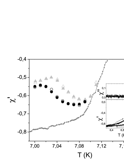
Figure 1: (Inset) Typical $\chi^{,,}$ and $\chi^{,}$ FCC and FCW curves in the linear regime measured at $f\,=\,30\,kHz$. Arrows indicate the direction of temperature variation. (Main panel) Zoom of the region delimited in the inset. Gray triangles (black circles) correspond to shaking frequency $f_{sh}\,=\,100\,kHz$ ($f_{sh}\,=\,10\,Hz$). Open (full) symbols for warming (cooling) experiment. In darkgray small circles a FCC curve is shown.

Figure 1 shows $\chi^{,}(T)$ measured in the linear regime ($h_{a}\,=\,0.025\,Oe$, $f\,=\,30\,kHz$), in a dc field $H\,=\,320\,Oe$ after different thermal and dynamical histories. In the Inset, both components $\chi^{,}$ and $\chi^{,,}$ in field cool cooling (FCC) and field cool warming (FCW) processes are shown in the full temperature range, and the region of the PE (main panel) is indicated. The curve with small darkgray circles in the main panel was obtained in a FCC process, where the VL remains trapped in a metastable disordered and strong pinned configuration, and the PE disappears. The other experimental points have been obtained by measuring the system after shaking the VL  at different frequencies. In all those cases, the following procedure has been performed: The system has been stabilized at a shaking temperature $T_{sh}$ and measured in the linear regime, recording the $\chi^{,}$ value corresponding to the starting configuration. Then the measurement was interrupted and $N_{sh}$ cycles of a sinusoidal shaking ac field ($h_{sh}\,=\,3.2\,Oe$) were applied. After switching off the shaking field, $\chi^{,}$ corresponding to the final value was recorded in the linear regime; then the system was driven to the next shaking temperature. Full and open symbols correspond to procedures increasing and decreasing $T_{sh}$. For clarity, in this figure only the final values are shown. Gray triangles indicate the response after shaking the system with $N_{sh}=100$ cycles at a frequency $f_{sh}\,=\,100\,kHz$, whereas black circles show the response after a similar procedure at $f_{sh}\,=\,10\,Hz$. One remarkable feature published in our previous work pasquini08 is that the final VLCs do not show appreciable relaxation (within our experimental time window) and are independent on the initial condition. Surprisingly, we find that these final states are not unique: they depend on the shaking frequency, but however the independence of initial conditions persists.

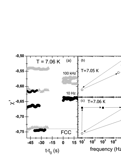
Figure 2: (a) $\chi^{,}$ versus time before and after shaking the system (the shaking time is not in scale and it is indicated by a gap without data). Gray (black) symbol correspond to $f_{sh}\,=\,100\,kHz$ ($f_{sh}\,=\,10\,Hz$ ). (b) $\chi^{,}$ values versus the shaking frequency (log scale). Arrows point from the values of $\chi^{,}$ before shaking to the values obtained after shaking. (c) $\chi^{,}$ values versus the fundamental shaking frequency for sinusoidal (open dots) and square (black squares) shaking waveforms.

In Fig. 2(a), the response at fixed temperature, before and after applying shaking protocols, is shown for different starting VLCs (same frequencies as in Fig. 1). It can be seen that the shaking field can order or disorder the VL. The various curves $\chi^{,}(t)$ obtained at different initial configurations collapse in an unique curve after shaking the system at a given frequency. Figure 2(b) shows the response after applying sinusoidal shaking fields at various frequencies. Arrows point from each starting VLC to the corresponding final configuration after shaking. In all the cases the final response is independent of the initial one, for shaking amplitudes greater than 1.8 Oe and above a number of applied cycles (in our system $N_{sh}\gtrapprox$ $40$). For all the tested frequencies (not all shown in the figure), the higher the shaking frequency, the more ordered the resulting VLC, consistent with a dynamic reordering of the VL reichhardt06 .

In that scenario, the frequency dependence would be due mainly to the different vortex velocities (i. e. forces) induced by the different shaking ac fields. Additional evidence supporting this fact arises from the response of the system to shaking fields with a square waveform. In this case it is expected that vortices move at higher velocities during short time intervals triggered and determined by the rising and falling edges, whereas the shaking frequency only modifies the waiting time between these short intervals. In Fig 2(c), it is seen that for square shaking fields, the VLCs are maximally ordered. On the other hand, frequency independence shows that relaxation processes are not relevant at least in this time window. As another evidence, we have confirmed that triangular and sinusoidal shaking fields (that at the same fundamental frequency induce similar vortex velocities) produce similar results.

The simulated system describes a very small region of the real macroscopic sample, where the mean vortex density and mean current density can be assumed to be homogeneous. In the experiment, the shaking ac field induces macroscopic currents $J_{sh}(t)$ that move vortices, that have been introduced in our simulations by a Lorentz force term $F^{L}=\phi_{0}J_{sh}\times\widehat{z}$, where $\widehat{z}$ is the versor parallel to the vortex direction. The explicit functional relation between $J_{sh}(t)$ and the shaking $h_{ac}(t)$ is not straightforward. In order to gain some intuition, we have applied the method developed in Ref. brandt, to obtain the distribution of $J(t)$ for a certain geometry, assuming a non linear electric field-current constitutive relation $E(J)=E_{c}(J/J_{c})^{n}$ nota . We have chosen a simple geometry (a disk) and we have estimated $n$ by comparing non linear susceptibility measurements and polar plots of $\chi^{,,}$ vs $\chi^{,}$. Under this non linear regime, given an external $h_{sh}(t)=h_{sh}\cos(\omega t)$ the current throughout most of the sample can be described by a square waveform of frequency $\omega$ and normalized amplitude $J_{0}(\omega)/J_{c}\gtrsim 1$ (Fig. 3(a)), being the frequency dependence logarithmic. Thus as a first (and very crude) approximation we will simulate our model with $J_{sh}(t)=J_{0}(\omega)\mbox{Sign}(\sin(\omega t))$.

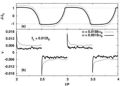
Figure 3: (a) Theoretical current density $J/J_{c}$ at a fixed position, in a superconducting disk of radius $a$ and a perpendicular sinusoidal magnetic field, as a function of $t/P$ for two different frequencies, 1$\tilde{\omega}$, solid line and 100$\tilde{\omega}$, dashed line, $\tilde{\omega}=\frac{2\pi E_{c}}{\mu_{0}aJ_{c}}$. Throughout most of the sample, the current can be described by a square waveform. (b) Calculated vortex mean velocity v, obtained from molecular dynamic simulations, as a function of $t/P$.

In our simulations, we consider $N_{v}$ rigid vortices with coordinates $\mathbf{r}_{i}$ in a two-dimensional rectangle of size $L_{x}\times L_{y}$ that evolve according to the dynamics $\eta\mathbf{v}_{i}=\mathbf{F}_{i}^{vv}+\mathbf{F}_{i}^{vp}+\mathbf{F}^{L},$ where $\mathbf{v}_{i}$ its velocity, $\eta$ the Bardeen-Stephen viscosity coefficient, $\mathbf{F}_{i}^{vv}=\sum_{j\neq i}^{N_{v}}f_{0}f_{vv}K_{1}(\frac{\mid\mathbf{r}_{i}-\mathbf{r}_{j}\mid}{\lambda})\hat{\mathbf{r}}_{ij}$ is the vortex-vortex interaction and $\mathbf{F}_{i}^{vp}=-\sum_{k=1}^{N_{p}}F_{k}^{p}e^{-(\frac{|r_{i}-R_{k}|}{r_{p}})^{2}}({\mathbf{r}}_{i}-{\mathbf{R}}_{k})$ is the pinning attraction. Here, $\phi_{0}$ is the quantum of magnetic flux, $\lambda$ is the London penetration length, $K_{1}$ is the special Bessel function and $f_{vv}$ is a dimensionless parameter that can be related to the stiffness of the vortex lattice. The $N_{p}$ pinning centers are located at random positions $\mathbf{R}_{k}$, with strength and range $F_{k}^{p}$ and $r_{p}$.We measure lengths in units of $\lambda$, forces (per unit length) in units of $f_{0}=\frac{\phi_{0}^{2}}{8\pi^{2}\lambda^{3}}$, time in units of $t_{0}=\eta\lambda/f_{0}$. We will consider $N_{v}=1600$, $L_{x}=40\lambda$, $L_{y}=\sqrt{3}L_{x}/2$, $N_{p}=25N_{v}$, $r_{p}=0.2\lambda$ and $F_{k}^{p}$ chosen from a Gaussian distribution with mean value $F^{p}=0.2$ and a standard deviation of $0.01F^{p}$. The equations of motion are integrated using a standard Euler algorithm with step $h=0.04t_{0}$, and a hard cut-off $\Lambda=4\lambda$ for the vortex-vortex force. The mean vortex velocity is defined as $\text{v}(t)=\frac{1}{N_{v}}\sum_{i}^{N_{v}}\text{v}_{i}(t)$, where $\text{v}_{i}(t)$ is the instantaneous velocity of the i-vortex in the force direction. The observable used to characterize the degree of order is the proportion of vortices with 6 neighbors $P_{6}=1-n_{d}$, where $n_{d}$ is the density of disclinations. $P_{6}$ is calculated at the end of each cycle.

We assume that the main effect of temperature near the PE is the increase of the ratio $f_{vp}/f_{vv}$, causing a spontaneous disordering of the VL. In the simulations, starting with a perfect ordered lattice (i. e. $P_{6}=1$) and leading the system to evolve without any applied external force, there is a spontaneous creation of disclinations, and a decrease in $P_{6}$. In the inset of Fig. 4, the spontaneous $P_{6}$ starting from an ordered configuration is plotted as a function of $f_{vp}/f_{vv}$. We identify the parameters corresponding to the experimental temperature region shown in Fig. 1 as the range where the VL spontaneously disorders. Therefore, we set the ratio $f_{vp}/f_{vv}=0.25$ to simulate the experimental system at a fixed temperature (experiments of Fig. 2). The dc depinning force per unit length $F_{c}^{dc}=\phi_{0}J_{c}\approx 0.01f_{0}$ was obtained by increasing a dc $F_{L}$ until the mean velocity $v$ exceeds a ”criterion voltage”. The shaking frequencies have been selected in the low frequency regime ($\omega<<\omega_{c}\sim\frac{\alpha_{L}}{\eta}\sim 0.11$) diego , where pinning forces dominate over viscous drags, because the experimental shaking frequencies are well below $f_{c}=\omega_{c}/2\pi>1MHz$

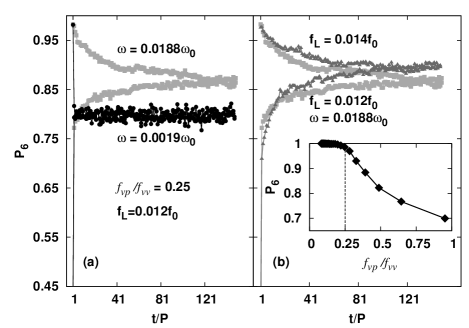
Figure 4: $P_{6}$ versus $t/P$ starting from an ordered and a disordered configuration. (a) For two different $\omega$ and fixed $f_{L}$. (b) For two different $f_{L}$ and fixed $\omega$. (Inset) $P_{6}$ versus $f_{vp}/f_{vv}$, showing a spontaneous creation of disclinations, and a decrease in $P_{6}$ at around $f_{vp}/f_{vv}=0.25$.

Figure 3(b) shows the calculated mean velocity as a function of time during two shaking cycles for two different frequencies. After switching the force direction, v decays towards a steady regime characteristic of a dc driving force, similar to that reported in Ref. reichhardt, that could be associated to a FSS. The transient time $\tau$ and the final mean velocity depend on the shaking force. At very low frequencies, the system reaches the steady regime inside each cycle (black curves in Fig. 3(b)) , and the response is essentially dc. This is not the case at higher frequencies (gray curve), were we observe that both $\tau$ and the final mean velocity slightly vary while the system evolves from a cycle to the next one. This fact is more clear in Fig. 4, that shows $P_{6}$ as a function of the number of cycles of the shaking force, starting from different initial conditions, at a fixed amplitude and two different frequencies (4(a)) and a fixed frequency and two amplitudes slightly above the depinning force (4(b)). After a new transient time $\tau_{ac}$, that can involve many shaking cycles, the disclination density remains fluctuating around a steady value, in a dynamic state independent of the initial condition, that depends on the amplitude of the shaking force.  When the force is very near the dc depinning force, a clear frequency dependence is also observed (Fig. 4(a)). It becomes clear that the higher the shaking frequency and amplitude of the shaking force (both effects expected by increasing, in the experiment, the frequency of a shaking field), the more ordered the resulting VLC, in agreement with that observed in our experiments. In this process, there are two different transient times that involve the creation or annihilation of disclinations: the characteristic dc time to decay to the FSS inside a cycle $\tau$ ( probably related with the experimental transient time $\tau_{2}$ in Ref. vortex2,  ) and the transient time $\tau_{ac}$ that can take many shaking cycles and could be related with the transient response observed in ac transport experiments vortex2 ; andrei . This second process is inherent of an oscillatory drive, and dynamically reorganizes the system in a VLC independent of the initial conditions.

In conclusion, a dynamic reorganization in the plastic regime that keeps memory of the frequency drive has been observed experimentally and numerically. Throughout the order disorder crossing phase boundary in $NbSe_{2}$ there is a large collection of VLCs, that can be accessed after the application of ac shaking fields of different frequency, either ordering or disordering the initial state. The order of the VLCs is determined by non invasive ac susceptibility measurements, showing that higher shaking frequencies lead to more ordered VLCs. The system forgets the initial condition and but keeps memory of the shaking frequency, suggesting that the nature of the final states is more complex than previously conjectured pasquini08 . Molecular dynamics simulations performed for a compatible set of interaction parameters in the plastic regime have reproduced qualitatively the salient features of experimental shaking protocols, revealing a plausible nature of the experimental VLCs. The dynamic steady states are reminiscent of FSS observed in other systems, as VL disclinations and mean vortex velocity fluctuate around a steady value. As a novel fact, we have identified two characteristic time constants: one characteristic of the dynamics inside each cycle (dc) and the second related to ac dynamics. Furthermore, as the theoretical model is similar to the one used in the simulations of other interacting systems reichhardt , we expect that frequency dependent final states should be observed experimentally in a wide collection of particle systems with plastic flow regimes. A deeper study of the transient processes and its connection with the depinning transition will be object of future work.

We thank E. Zeldov for useful discussions. This work was supported by UBACyT, ANPCyT and CONICET.

References

- (1) N. Mangan, C. Reichhardt and C. J. Olson Reichhardt, Phys. Rev. Lett. 100, 187002 (2008).
- (2) S. Okuma, Y. Tsugawa, and A. Motohashi, Phys. Rev. B 83, 012503 (2011).
- (3) T. Giamarchi and P. Le Doussal, Phys. Rev. Lett. 72, 1530 (1994); Phys. Rev. B 52,1242 (1995).
- (4) A. E. Koshelev and V. M. Vinokur, Phys. Rev. Lett. 73, 3580 (1994).
- (5) A. B. Pippard, Proc. R. Soc. A 216, 547 (1953).
- (6) W. Henderson , E. Y. Andrei, and M. J. Higgins Phys. Rev. Lett. 81, 2352 (1998).
- (7) Y. Paltiel, E. Zeldov, Y. Myasoedov, M. L. Rappaport, G. Jung, S. Bhattacharya, M. J. Higgins, Z. Xiao, E. Y. Andrei, P. L. Gammel, and D. J. Bishop, Phys. Rev. Lett. 85, 3712 (2000).
- (8) Z. L. Xiao, O. Dogru, E. Y. Andrei, P. Shuk, and M. Greenblatt, Phys. Rev. Lett. 92, 227004 (2004).
- (9) G. Pasquini, D. Pérez Daroca, C. Chiliotte, G. S. Lozano, and V. Bekeris, Phys. Rev. Lett. 100, 247003 (2008).
- (10) D. Pérez Daroca, G. S. Lozano, G. Pasquini, and V. Bekeris, Phys. Rev. B 81, 184520 (2010).
- (11) C. Reichhardt and C. J. Olson, Phys. Rev. E 73, 046122 (2006).
- (12) S. Cox, J. Singleton, R. D. McDonald, A. Migliori, and P. B. Littlewood, Nature Materials 7, 25 (2008).
- (13) A. Pertsinidis and X. S. Ling, Phys. Rev. Lett. 100, 028303 (2008).
- (14) C. Reichhardt and C. J. Olson, Phys. Rev. Lett. 103, 168301 (2009).
- (15) L. Corté, P. M. Chaikin, J. P. Gollub and D. J. Pine, Nature Phys. 4, 420 (2008).
- (16) Z.-X. Gong, G.-D. Lin, and L.-M. Duan, Phys. Rev. Lett. 105, 265703 (2010).
- (17) D. Ilgaz et al., Phys. Rev. Lett. 105, 076601 (2010).
- (18) E. H. Brandt, Phys. Rev. B 50, 4034 (1994).
- (19) Crystal provided by Bell Labs, grown as in C. S. Oglesby, E. Bucher, C. Kloc, and H. Hohl, J. Crys. Growth 137, 289 (1994).
- (20) Similar qualitative response was observed in other crystals grown as in I. Guillamon, H. Suderow, S. Vieira, L. Cario, P. Diener, and P. Rodiere, Phys. Rev. Lett. 101, 166407 (2008).
- (21) U. Yaron, P. L. Gammel, D. A. huse, R. N. Kleiman, C. S. Oglesby, E. Bucher, B. Batlogg, and D. J. Bishop, Phys. Rev. Lett. 73, 2748 (1994).
- (22) A. I. Larkin and Yu N. Ovchinnikov, J. Low Temp. Phys. 34, 409 (1979).
- (23) A. M. Campbell, J. Phys. C 4, 3186 (1971).
- (24) G. Pasquini, L. Civale, H. Lanza, and G. Nieva, Phys. Rev B. 59, 9627 (1999), and references therein.
- (25) As we are dealing with a low superconductor and creep is negligible, a very large has been set for .