Subspace Properties of Network Coding
and their Applications

Abstract

Systems that employ network coding for content distribution convey to the receivers linear combinations of the source packets. If we assume randomized network coding, during this process the network nodes collect random subspaces of the space spanned by the source packets. We establish several fundamental properties of the random subspaces induced in such a system, and show that these subspaces implicitly carry topological information about the network and its state that can be passively collected and inferred. We leverage this information towards a number of applications that are interesting in their own right, such as topology inference, bottleneck discovery in peer-to-peer systems and locating Byzantine attackers. We thus argue that, randomized network coding, apart from its better known properties for improving information delivery rate, can additionally facilitate network management and control.

I Introduction

Randomized network coding offers a promising technique for content distribution systems. In randomized network coding, each node in the network combines its incoming packets randomly and sends them to its neighbours [1, 2]. This is the approach adopted by most practical applications today. For example, Avalanche, the first implementation of a peer-to-peer (P2P) system that uses network coding, adopts such a randomized operation [3, 4]. In ad-hoc wireless and sensor networks as well, most proposed protocols employing network coding again opt for randomized network operation (see [9] and references therein).

The reason for the popularity of randomized network coding is because it facilitates a very simple and flexible network operation without need of synchronization among network nodes, that is well suited to packet networks. To every packet, a coding vector is appended that determines how the packet is expressed with respect to the original data packets produced at the source node. When intermediate nodes combine packets, the coding vector keeps track of the linear combinations contained in a particular packet. A receiver which collects enough packets, uses the coding vectors to determine the set of linear equations it needs to solve in order to recover the original data packets.

Our contributions start with the observation that coding vectors implicitly carry information about the network structure as well as its state. Such vectors belong to appropriately defined vector spaces, and we are interested in fundamental properties of these (finite-field) vector spaces. In particular, since we are investigating properties induced by randomized network coding, we need to characterize random subspaces of the aforementioned vector spaces. These properties of random subspaces over finite fields might be of independent interest. We aim to show, using these properties, that observing the coding vectors we can passively collect structural and state information about a network. We can leverage this information towards several applications that are interesting in their own merit, such as topology inference, network tomography, and network management (we do not claim here the design of practical protocols that use these properties). However, we show that randomized network coding, apart from its better known properties for facilitating information delivery, can provide us with information about the network itself.

To support this claim, we start by studying the problem of passive topology inference in a content distribution system where intermediate nodes perform randomized network coding. We show that the subspaces nodes collect during the dissemination process have a dependence with each other which is inherited from the network structure. Using this dependence, we describe the conditions that let us perfectly reconstruct the topology of a network, if subspaces of all nodes at some time instant are available.

We then investigate a reverse or dual problem of topology inference, which is, finding the location of Byzantine attackers. In a network coded system, the adversarial nodes in the network can disrupt the normal operation of information flow by inserting erroneous packets into the network. We use the dependence between subspaces gathered by network nodes and the topology of the network to extract information about the location of attackers. We propose several methods, compare them and investigate the conditions that allow us to find the location of attackers up to a small uncertainty.

Finally, we then observe that the received subspaces, even at one specific node, reveal some information about the network, such as the existence of bottlenecks or congestion. We consider P2P networks for content distribution that use randomized network coding techniques. It is known that the performance of such P2P networks depends critically on the good connectivity of the overlay topology. Building on our observation, we propose algorithms for topology management to avoid bottlenecks and clustering in network-coded P2P systems. The proposed approach is decentralized, inherently adapts to the network topology, and reduces substantially the number of topology rewirings that are necessary to maintain a well connected overlay; moreover, it is integrated in the normal content distribution.

The paper is organized as follows. We start with the notation and problem modeling in §II. We investigate the properties of vector spaces in a system that employs randomized network coding in §III and these properties give the framework to explore applications in §IV, §V, and §VI. Finally, we conclude the paper with a discussion in §VII. Shorter versions of these results have also appeared in [10, 11, 12].

I-A Related Work

Network coding started by the work of Ahlswede et al. [13] who showed that a source can multicast information at a rate approaching the smallest min-cut between the source and any receiver if the middle nodes in the network combine the information packets. Li et al. [14] showed that linear network coding with finite field size is sufficient for multicast. Koetter et al. [15] presented an algebraic framework for linear network coding.

Randomized network coding was proposed by Ho et al. [16] where they showed that randomly choosing the network code leads to a valid solution for a multicast problem with high probability if the field size is large. It was later applied by Chou et al. [2] to demonstrate the practical aspects of random linear network coding. Gkantsidis et al. [3, 4] implemented a practical file sharing system based on this idea. Several other works have also adopted randomized network coding for content distribution, see for example [5, 6, 7].

Network error correcting codes, that are capable of correcting errors inserted in the network, have been developed during the last few years. For example see the work of Koetter et al. [17], Jaggi et al. [18], Ho et al. [19], Yeung et al. [20, 21], Zhang [22], and Silva et al. [23]. These schemes are capable of delivering information despite the presence of Byzantine attacks in the network or nodes malfunction, as long as the amount of undesired information is limited. These network error correcting schemes allow to correct malicious packet corruption up to certain rate. In contrast, we use network coding to identify malicious nodes in our work. Recently, and following our work [12], additional approaches are proposed in the literature, some building on our results [24].

Overlay topology monitoring and management that do not employ network coding has been an intensively studied research topic, see for example [25]. However, in the context of network coding, it is a new area of research. Fragouli et al. [26, 27] took advantage of network coding capabilities for active link loss network monitoring where the focus was on link loss rate inference. Passive inference of link loss rates has also been proposed by Ho et al. [28]. In a subsequent work of ours, Sharma et al. [29] study passive topology estimation for the upstream nodes of every network node. This work is based on the assumption that the local coding vectors for each node in the network are fixed, generated in advance and known by all other nodes in the network, unlike our work that builds on randomized operation. The idea of passive inference of topological properties from subspaces that are build over time, as far as we know, is a novel contribution of this work.

II Models: Coding and Network Operation

A simple observation motivates much of the work presented in this paper: the subspaces gathered by the network nodes during information dissemination with randomized network coding, are not completely random, but have some relationship, and this relationship conveys information about the network topology as well as its state. We will thus investigate properties of the collected subspaces and show how we can use them for diverse applications.

Different properties of the subspaces are relevant to each particular application and therefore we will develop a framework for investigating these properties. This will also involve some understanding of modeling the problem to fit the requirements of an application and then developing subspace properties relevant to that model.

II-A Notation

Let $q\geq 2$ be a power of a prime. In this paper, all vectors and matrices have elements in a finite field $\mathbb{F}_{q}$. We use $\mathbb{F}^{n\times m}_{q}$ to denote the set of all $n\times m$ matrices over $\mathbb{F}_{q}$, and $\mathbb{F}^{\ell}_{q}$ to denote the set of all row vectors of length $\ell$. The set $\mathbb{F}^{\ell}_{q}$ forms an $\ell$-dimensional vector space over the field $\mathbb{F}_{q}$. Note that all vectors are row vectors unless otherwise stated. Bold lower-case letters, e.g., $\boldsymbol{v}$, are used for vectors and bold capital letters, e.g., $\boldsymbol{X}$, are used to denote matrices.

For a set of vectors $\{\boldsymbol{v}_{1},\ldots,\boldsymbol{v}_{k}\}$ we denote their linear span by $\left\langle\boldsymbol{v}_{1},\ldots,\boldsymbol{v}_{k}\right\rangle$. For a matrix $\boldsymbol{X}$, $\left\langle\boldsymbol{X}\right\rangle$ is the subspace spanned by the rows of $\boldsymbol{X}$. We then have $\operatorname{rank}(\boldsymbol{X})=\dim(\left\langle\boldsymbol{X}\right\rangle)$.

We denote subspaces of a vector space by $\Pi$ and sometimes also by $\pi$. In this paper, we work on a vector space $\mathbb{F}_{q}^{\ell}$ of dimension $\ell$ defined over a finite field $\mathbb{F}_{q}$. For two subspaces $\Pi_{1},\Pi_{2}\subseteq\mathbb{F}_{q}^{\ell}$, we will denote their intersection by $\Pi_{1}\cap\Pi_{2}$ and their joint span by $\Pi_{1}+\Pi_{2}$ where

$$\Pi_{1}+\Pi_{2}\triangleq\{\boldsymbol{v}_{1}+\boldsymbol{v}_{2}|\boldsymbol{v}_{1}\in\Pi_{1},\boldsymbol{v}_{2}\in\Pi_{2}\},$$

is the smallest subspace that contains both $\Pi_{1}$ and $\Pi_{2}$. It is well known that

$$\dim(\Pi_{1}+\Pi_{2})=\dim(\Pi_{1})+\dim(\Pi_{2})-\dim(\Pi_{1}\cap\Pi_{2}).$$

We also use the following metric to measure the distance between two subspaces,

$$d_{S}(\Pi_{1},\Pi_{2}) \triangleq\dim(\Pi_{1}+\Pi_{2})-\dim(\Pi_{1}\cap\Pi_{2})$$ (1)

$$=\dim(\Pi_{1})+\dim(\Pi_{2})-2\dim(\Pi_{1}\cap\Pi_{2}).$$

This metric was also introduced in [17], where it was used to design error correction codes.

In addition to the metric $d_{S}(\cdot,\cdot)$ defined above, in some cases we will also need a measure that compares how a set $\mathcal{A}$ of subspaces differs from another set $\mathcal{B}$ of subspaces. For this we will use the average pair-wise distance defined as follows

$$D_{S}(\mathcal{A},\mathcal{B})\triangleq\frac{1}{|\mathcal{A}||\mathcal{B}|}\sum_{\pi_{a}\in\mathcal{A},\pi_{b}\in\mathcal{B}}d_{S}(\pi_{a},\pi_{b}).$$ (2)

It should be noted that the above relation does not define a metric for the set of subspaces because the self distance of a set with itself is not zero. However, $D_{S}(\cdot,\cdot)$ satisfies the triangle inequality.

In this paper we will be interested in investigating the relationship of the collected subspaces at neighboring network nodes. We consider a network represented as a directed acyclic graph $G=(V,E)$, with $\vartheta=|V|$ nodes and $\xi=|E|$ edges. For an arbitrary edge $e=(u,v)\in E$, we denote $\operatorname{head}(e)=v$ and $\operatorname{tail}(e)=u$. For an arbitrary node $v\in V$, we denote $\operatorname{In}(v)$ the set of incoming edges to $v$ and $\operatorname{Out}(v)$ the set of outgoing edges from $v$. If a node $u$ has $p$ parents $u_{1},\ldots,u_{p}$, we denote with $P(u)=\{u_{1},\ldots,u_{p}\}$ the set of parents of $u$. We use $P^{l}(u)$ to denote the set of all ancestors of $u$ at distance $l$ from $u$ in the network (we say that two nodes $u$ and $v$ are at distance $l$ if there exists a path of length exactly $l$ that connects them). We denote with $\pi^{(u_{i})}_{u}(t)$ the subspace node $u$ receives from parent $u_{i}$ at exactly time $t$, and with $\pi_{u}(t)$ the whole subspace (from all parents) that node $u$ receives at time $t$, that is $\pi_{u}(t)=\sum_{i=1}^{p}\pi_{u}^{(u_{i})}(t)$. We also denote with $\Pi^{(u_{i})}_{u}(t)$ the subspace node $u$ has received from parent $u_{i}$ up to time $t$, that is, $\Pi^{(u_{i})}_{u}(t)=\Pi^{(u_{i})}_{u}(t-1)+\pi^{(u_{i})}_{u}(t)$. Then the subspace $\Pi_{u}(t)$ that the node has at time $t$ can be expressed as $\Pi_{u}(t)=\sum_{i=1}^{p}\Pi^{(u_{i})}_{u}(t)$. For a set of nodes $\mathcal{U}=\{u_{1},\ldots,u_{p}\}$, we define $\Pi_{\mathcal{U}}=\Pi_{u_{1}}+\cdots+\Pi_{u_{p}}$.

Finally, we use the big $O$ notation which is defined as follows. Let $f(x)$ and $g(x)$ be two functions defined on some subset of the real numbers. We write $f(x)=O(g(x))$ if and only if there exists a positive real number $M$ and a real number $x_{0}$ such that $|f(x)|\leq M|g(x)|$ for all $x>x_{0}$. During the rest of the paper we use $O$ to compare functions of the field size $q$, unless otherwise stated. For example, we will use $f(q)=O(q^{-1})$ to imply that the value of $f(q)$ goes to zero as $q^{-1}$ for $q\rightarrow\infty$.

II-B Network Operation

We assume that there is an information source located on a node $S$ that has a set of $n$ packets (messages) $\{\boldsymbol{x}_{1},\ldots,\boldsymbol{x}_{n}\}$, $\boldsymbol{x}_{i}\in\mathbb{F}_{q}^{\ell}$, to distribute to a set of receivers, where each packet is a sequence of $\ell$ symbols over the finite field $\mathbb{F}_{q}$. To do so, we will employ a dissemination protocol based on randomized network coding, namely, where each network node sends random linear combinations (chosen to be uniform over $\mathbb{F}_{q}$) of its collected packets to its neighbors. We assume for simplicity that there are no packet-losses.

Dissemination Protocol

It is possible to separate the dissemination protocols into the following operation categories.

• Synchronous: All nodes are synchronized and transmit to their neighbors according to a global clock tick (time-slot). At timeslot $t\in\mathbb{N}$, node $v$ sends linear combinations from all vectors it has collected up to time $t-1$. Once nodes start transmitting information, they keep transmitting until all receivers are able to decode.

• Asynchronous: Nodes transmit linear combinations at randomly and independently chosen time instants.

In this paper, we focus on the synchronous network where we assume that each link has unit delay corresponding to each timeslot, however our results can be extended to asynchronous networks as well.

Next, we explain in detail the dissemination protocol, that is summarized in Algorithm II.

Timing

We depict in Fig. 1 the relative timing of events within a timeslot. Nodes transmit at the beginning of a timeslot. We assume that each packet is received by its intended receiver before the end of the timeslot. Thus, the timeslot duration incorporates the packet propagation delay in one edge of the network.

Figure 1: Timing schedule of the dissemination protocol given by Algorithm II.

Rate Allocation and Equivalent Network Graph

The dissemination protocol first associates with each link $e$ of the network a rate $r_{e}$ (measured as the number of packets transmitted per timeslot on edge $e$). These rates are selected in advance using a rate allocation method, for example [8].

For the rest of the paper, we consider an equivalent network graph, where each edge $e$ has capacity equal to its allocated rate $r_{e}$. On this new graph, we can define the min-cut $c_{v}$ from the source node $S$ to a node $v\in V$. Whenever we refer to min-cut values in the following, we imply min-cut values over this equivalent graph.

We assume that the rate allocation protocol we use satisfies

$$r_{e}\leq\min[c_{e},c_{\operatorname{tail}(e)}],$$ (3)

where $c_{e}$ is the capacity of edge $e$. This very mild assumption says that the node $v=\operatorname{tail}(e)$ does not send more information than it receives, and is satisfied by all protocols that do not send redundant packets, i.e., observe flow conservation.

In our work, we consider the case where $n\gg c_{v}$, namely, the dissemination of the $n$ source packets to the receivers takes place by using the network over several timeslots.

Node operation

When the dissemination starts, at timeslot say zero, the source starts transmitting at each time slot and to each of its outgoing edges $e$, $r_{e}$ randomly selected linear combinations of $n$ information packets. We will call $r_{S}$ the source rate. The source continues until it has transmitted linear combinations of all $n$ packets, i.e., for $\frac{n}{r_{S}}$ timeslots. Every other node $v\in V\setminus\{S\}$ in the network, operates as follows:

• Initially it does not transmit, but only collects in a buffer packets from its parents, until a time $\tau_{v}$, which we call waiting time and we will define in the following. As we will see, each node can decide the waiting time by itself and independently from other nodes.

• At each timeslot $t$, for all $t\geq\tau_{v}+1$, it transmits to each outgoing edge $e$, $r_{e}$ linear combinations of all packets it has collected in its buffer up to time $t-1$.

Collected Subspaces

We can think of each of the $n$ source messages $\{\boldsymbol{x}_{i}\}$ as corresponding to one dimension of an $n$-dimensional space $\Pi_{S}\subseteq\mathbb{F}_{q}^{\ell}$ where $\Pi_{S}=\left\langle\boldsymbol{x}_{1},\ldots,\boldsymbol{x}_{n}\right\rangle$. We say that node $v\in V$ at time $t$ observes a subspace $\Pi_{v}(t)\subseteq\Pi_{S}$, with dimension $d_{v}(t)\triangleq\dim(\Pi_{v}(t))$, if $\Pi_{v}(t)$ is the space spanned by the received vectors at node $v$ up to time $t$. Initially, at time $t=0$, the collected subspaces of all nodes (apart the source) are empty; $d_{v}(0)=0$, $\forall v\in V\setminus\{S\}$.

Waiting Times

We next define the waiting times, that will be used in the following sections to ensure that the subspaces of different nodes be distinct, and are a usual assumption in dissemination protocols; indeed, for large $n$ the waiting time does not affect the rate. For example, in the information-theoretic proof of the main theorem in network coding [13], each node waits until it collects at least one message from each of its incoming links before starting transmissions.

Definition 1

The waiting time $\tau_{v}$ for a node $v$ is the first timeslot during which node $v$ receives information from the source at a rate equal to its min-cut $c_{v}$, and additionally, has collected in its buffer a subspace of dimension at least $c_{v}+1$.

Note that, because we are dealing with acyclic graphs, we can impose a partial order on the waiting times of the nodes, such that all parents of a node have smaller waiting time than the node. Moreover, each node can decide whether the conditions for the waiting time are met, by observing whether it receives information at a rate equal to its min-cut, and what is the dimension of the subspace it has collected. That is, a node does not need to know any topological information (apart from its min-cut), and the waiting times do not need to be communicated in advance to the nodes, but can be decided online based on the network conditions.

Algorithm II.1:  DisseminationProtocol($G=(V,E),S,n,\tau_{v},r_{e}$) $\begin{array}[]{@{\pcode@tab{1}}lr@{}}\hskip 4.30554pt\lx@intercol{}\mbox{for each }v\in V\setminus\{S\}\\ \hskip 4.30554pt\lx@intercol\hskip 4.30554pt\mbox{ do }\Pi_{v}(0)=\varnothing,d_{v}(0)=0\\ \hskip 4.30554pt\lx@intercol t\leftarrow 1\\ \hskip 4.30554pt\lx@intercol\mbox{while }\min_{v}{d_{v}(t)}<n\\ \hskip 4.30554pt\lx@intercol\left\{\begin{array}[]{@{}lr@{}}\mbox{for each }v\in V\\ \left\{\begin{array}[]{@{}lr@{}}\mbox{if }t\geq\tau_{v}+1\\ \hskip 4.30554pt\mbox{ then }\left\{\begin{array}[]{@{}lr@{}}\mbox{for each }e\in\operatorname{Out}(v)\\ \hskip 4.30554pt\mbox{ do }\left\{\begin{array}[]{@{}lr@{}}\text{node $v$ transmits from}\\ \text{$\Pi_{v}(t-1)$ with rate $r_{e}$ on $e$}\\ \end{array}\right.\end{array}\right.\end{array}\right.\\ \mbox{for each }v\in V\\ \hskip 4.30554pt\mbox{ do }\;\text{update}\;\Pi_{v}(t),\;d_{v}(t)\\ t\leftarrow t+1\\ \end{array}\right.\end{array}$

Alg. II: Dissemination protocol.

Source Operation and the Source Subspace $\Pi_{S}$

As we discussed, the source needs to convey to the receivers $n$ source packets that span the $n$-dimensional subspace $\Pi_{S}=\left\langle\boldsymbol{x}_{1},\ldots,\boldsymbol{x}_{n}\right\rangle$, with $\Pi_{S}\subseteq\mathbb{F}_{q}^{\ell}$. $\Pi_{S}$ is isomorphic to $\mathbb{F}_{q}^{n}$; thus, for the purpose of studying relationships between subspaces of $\Pi_{S}$, we can equivalently assume that $\Pi_{S}=\mathbb{F}_{q}^{n}$, and that node $v\in V$ at time $t$ observes a subspace $\Pi_{v}(t)\subseteq\Pi_{S}$. This simplification is very natural in the case where we employ coding vectors, reviewed briefly in the following, as we only need consider the coding vectors for our purposes and ignore the remaining contents of the packets; however, we can also use the same approach in the case where the source performs noncoherent coding, described subsequently.

Use of Coding Vectors

To enable receivers to decode, the source assigns $n$ symbols of each message vector (packet) to determine the linear relation between that packet and the original vectors $\boldsymbol{x}_{i}$, $i=1,\ldots,n$. Without loss of generality, let us assume these $n$ symbols (which form a vector of length $n$) are placed at the beginning of each message vector. This vector is called coding vector. Each message vector $\boldsymbol{x}_{i}$ contains two parts. The vector $\boldsymbol{x}_{i}^{C}\in\mathbb{F}_{q}^{n}$ with length $n$ is the coding vector and remaining part, $\boldsymbol{x}_{i}^{I}\in\mathbb{F}_{q}^{\ell-n}$, is the information part where

$$\boldsymbol{x}_{i}\triangleq[\boldsymbol{x}_{i}^{C}\ |\ \boldsymbol{x}_{i}^{I}].$$

The coding vectors $\boldsymbol{x}_{i}^{C}$, $i=1,\ldots,n$ are chosen such that they form a basis for $\mathbb{F}_{q}^{n}$. For simplicity we assume $\boldsymbol{x}_{i}^{C}=\boldsymbol{e}_{i}$ where $\boldsymbol{e}_{i}\in\mathbb{F}_{q}^{n}$ is a vector with one at position $i$ and zero elsewhere.

For our purposes, it is sufficient to restrict our algorithms to examine the coding vectors. Thus, the source has the space $\Pi_{S}=\mathbb{F}_{q}^{n}$; during the information dissemination, if a node $v$ at time $t$ has collected $m$ packets $\boldsymbol{z}_{i}$ with coding vectors $\boldsymbol{z}_{i}^{C}$, it has observed the subspace $\Pi_{v}(t)=\left\langle\boldsymbol{z}_{1}^{C},\ldots,\boldsymbol{z}_{m}^{C}\right\rangle$. In other words, the coding vectors capture all the information we need for our applications.

Subspace Coding

Our approach also works in the case of subspace coding, that was introduced in [17]. We next briefly explain the idea of communication using subspaces, in a network performing randomized network coding.

In the following, we use the same notation as introduced in §II-B. Let $\{\boldsymbol{x}_{1},\ldots,\boldsymbol{x}_{n}\}$, $\boldsymbol{x}_{i}\in\mathbb{F}_{q}^{\ell}$ denote the set of packets the source has. Assume that there is no error in the network. An arbitrary receiver $R_{v}$ at node $v$ collects $m$ packets $\boldsymbol{z}_{i}$, $i=1,\ldots,m$, where each $\boldsymbol{z}_{i}$ can be presented as $\boldsymbol{z}_{i}=\sum_{j=1}^{n}h_{ij}\boldsymbol{x}_{j}$. The coefficients $h_{ij}$ are unknown and randomly chosen over $\mathbb{F}_{q}$. In matrix form, the transmission model can be represented as

$$\boldsymbol{Z}_{v}=\boldsymbol{H}_{Sv}\boldsymbol{X},$$

where $\boldsymbol{H}_{Sv}\in\mathbb{F}_{q}^{m\times n}$ is a random matrix and $\boldsymbol{X}\in\mathbb{F}_{q}^{n\times\ell}$ is the matrix whose rows are the sources’ packets.

The matrices $\boldsymbol{H}_{Sv}$ are randomly chosen, under constraints imposed by the network topology. As stated in [17] and proved in [30, 31, 32], the above model naturally leads to consider information transmission not via the choice of $\boldsymbol{x}_{i}$ but rather by the choice of the vector space spanned by $\{\boldsymbol{x}_{i}\}$.

In the case of subspace coding, the dissemination algorithm works in exactly the same way as in the case of coding vectors; what changes is how the source maps the information to the packets it transmits, and how decoding occurs. However, this is orthogonal to our purposes, since we perform no decoding of the information messages, but simply observe the relationship between the subspaces different nodes in the network collect. Thus, the same approach can be applied in this case as well.

II-C Input to Algorithms

We are interested in designing algorithms that leverage the relationships between subspaces observed at different network nodes for network management and control. The algorithms design will depend on the information that we have access to. We distinguish between the following.

• Global information: A central entity knows the subspaces that all $\vartheta$ nodes in the network have observed.

• Local Information: There is no such omniscient entity, and each node $v$ only knows what it has received, its own subspace $\Pi_{v}$.

We may also have information between these two extreme cases. Moreover, we may have a static view, where we take a snapshot of the network at a given time instant $t$, or a non-static view, where we take several snapshots of the network and use the subspaces’ evolution to design an algorithm.

We will argue in Section IV that capturing even global information can be accomplished with relatively low overhead (sending one additional packet per node at the end of the dissemination protocol); thus, the algorithms we develop even assuming global information can in fact be implemented almost passively and at low cost.

III Properties of Random Vector Spaces over a Finite Field $\mathbb{F}_{q}^{n}$

In this section, we will state and prove basic properties and results that we will exploit towards various applications in the following sections. In particular, we will investigate the properties of random sampling from vector spaces over a finite field. Such properties give us a better insight and understanding of randomized network coding and form a foundation for the results and algorithms presented in this paper.

III-A Sampling Subspaces over $\mathbb{F}_{q}^{n}$

Here, we explore properties of randomly sampled subspaces from a vector space $\mathbb{F}_{q}^{n}$. We start with the following lemma that explores properties of a single subspace.

Lemma 1

Suppose we choose $m$ vectors from an $n$-dimensional vector space $\Pi_{S}=\mathbb{F}_{q}^{n}$ uniformly at random to construct a space $\Pi$. Then the subspace $\Pi$ will be full rank (has dimension $\min[m,n]$) w.h.p. (with high probability), namely,

$${\mathbb{P}\left[\dim(\Pi)=\min[m,n]\right]}=[1-O\left(q^{-1}\right)].$$

Proof:

Refer to Appendix A. ∎

We conclude that for large values of $q$, selecting $m\leq n$ vectors uniformly at random from $\mathbb{F}_{q}^{n}$ to construct a subspace $\Pi$ is equivalent to choosing an $m$-dimensional subspace from $\mathbb{F}_{q}^{n}$ uniformly at random. Note that this is not true for small values of $q$.

We next examine connections between multiple subspaces.

Lemma 2

Let $\Pi_{1}$ and $\Pi_{2}$ be two subspaces of $\Pi_{S}=\mathbb{F}_{q}^{n}$ with dimension $d_{1}$ and $d_{2}$ respectively, intersection of dimension $d_{12}$ and $\Pi_{1}\nsubseteq\Pi_{2}$ (i.e., $d_{12}<d_{1}$). Construct $\Pi_{1}^{\prime}$ by choosing $m$ vectors from $\Pi_{1}$ uniformly at random. Then ${\mathbb{P}\left[\Pi_{1}^{\prime}\subset\Pi_{2}\right]}=O\left(q^{-m}\right).$

Proof:

Refer to Appendix A. ∎

Lemma 3

Suppose $\Pi_{k}$ is a $k$-dimensional subspace of a vector space $\Pi_{S}=\mathbb{F}_{q}^{n}$. Select $m$ vectors uniformly at random from $\Pi_{S}$ to construct the subspace $\Pi$. We have

$$\dim(\Pi\cap\Pi_{k}) = \min[k,(m-(n-k))^{+}]$$ (4)

$$= \left(\min[m,n]+k-n\right)^{+},$$

with probability $1-O\left(q^{-1}\right)$.

Proof:

Refer to Appendix A. ∎

Corollary 1

Suppose $\Pi_{1}$ and $\Pi_{2}$ are two subspace of $\mathbb{F}_{q}^{n}$ with dimension $d_{1}$ and $d_{2}$ respectively and joint dimension $d_{12}$. Let us take $m_{1}$ vectors uniformly at random from $\Pi_{1}$ and $m_{2}$ vectors from $\Pi_{2}$ to construct subspaces $\hat{\Pi}_{1}$ and $\hat{\Pi}_{2}$. We have

$$\dim(\hat{\Pi}_{1}\cap\hat{\Pi}_{2})= \min\left[d_{12},(m_{1}+m_{2}-(d_{1}+d_{2}-d_{12}))^{+},\right.$$

$$\left.(m_{1}-(d_{1}-d_{12}))^{+},(m_{2}-(d_{2}-d_{12}))^{+}\right],$$

with probability $1-O\left(q^{-1}\right)$.

Proof:

Refer to Appendix A. ∎

By choosing $\Pi_{1}=\Pi_{2}=\mathbb{F}_{q}^{n}$ in Corollary 1 we have the following corollary.

Corollary 2

Let us construct two subspaces $\hat{\Pi}_{1}$ and $\hat{\Pi}_{2}$ by choosing $m_{1}$ and $m_{2}$ vectors uniformly at random respectively from $\mathbb{F}_{q}^{n}$. Then the subspaces $\hat{\Pi}_{1}$ and $\hat{\Pi}_{2}$ will be disjoint with probability $1-O\left(q^{-1}\right)$ if $m_{1}+m_{2}\leq n$.

We are now ready to discuss one of the important properties of randomly chosen subspaces which is very useful for our work: randomly selected subspaces tend to be “as far as possible”. We will clarify and make precise what we mean by “as far as possible”, see also [33]. We first review the definition of a subspace in general position with respect to a family of subspaces.

Definition 2 ([33, Chapter 3])

Let $\Pi_{S}$ be an $n$-dimensional space over the field $\mathbb{F}_{q}$ and for $i=1,\ldots,r$, let $\Pi_{i}$ be a subspace of $\Pi_{S}$, with $\dim(\Pi_{i})=d_{i}$. A subspace $\Pi\subseteq\Pi_{S}$ of dimension $d$ is in general position with respect to the family $\{\Pi_{i}\}$ if

$$\dim(\Pi_{i}\cap\Pi)=\max\left[d_{i}+d-n,0\right],\quad\forall i\in\{1,\ldots,r\}.$$ (5)

It should be noted that $\max[d_{i}+d-n,0]$ is the minimum possible dimension of $(\Pi_{i}\cap\Pi)$. So what the above definition says is that the intersection of $\Pi$ and each $\Pi_{i}$ is as small as possible. Using the above definition we can state the following theorem.

Theorem 1

Suppose $\{\Pi_{i}\}$, $i=1,\ldots,r$, are subspaces of $\Pi_{S}=\mathbb{F}_{q}^{n}$. Let us construct a subspace $\Pi$ by randomly choosing $m$ vectors from $\Pi_{S}$. Then $\Pi$ will be in general position with respect to the family $\{\Pi_{i}\}$ w.h.p., i.e., with probability $1-O\left(q^{-1}\right)$.

Proof:

Refer to Appendix A. ∎

Theorem 1 demonstrates a nice property of randomized network coding where the subspaces spanned by coding vectors tend to be as far as possible on different paths of the network.

III-B Rate of Innovative Packets

In the following sections, we will need to know the rate of receiving innovative message vectors (packets) at receivers in a dissemination protocol performing randomized network coding. By innovative we refer to vectors that do not belong in the space spanned by already collected packets. As it is shown in [13], the source can multicast at rate equal to the minimum min-cut of all receivers if the intermediate nodes can combine the incoming messages. Moreover, it is shown in [14] that using linear combinations is sufficient to achieve information transfer at a rate equal to the minimum mincut of all receivers. In [13, 1], it is also demonstrated that choosing the coefficients of the linear combinations randomly is sufficient (no network-specific code design is required) with high probability if the field size is large enough.

To find the rate of receiving information at each node where the implemented dissemination protocol performs randomized network coding, we can use the following result given in Theorem 2. Note that our described dissemination protocol, although very common in practice, does not exactly fit to the previous theoretical results in the literature that examine rates, because the operation of the network nodes is not memory-less. That is, while for example in [1, 13, 14] each transmitted packet at time $t$ is a function of a small subset of the received packets up to time $t$ (the ones corresponding to the same information message), in our case a packet transmitted at time $t$ is a random linear combination of all packets received up to time $t$. This small variant of the main theorem on randomized network coding is very intuitive, and we formally state it in following.

Theorem 2

Consider a source that transmits $n$ packets over a connected network using the dissemination protocol described in §II-B, and assume that the network nodes perform random linear network coding over a sufficiently large finite field. Then there exists $t_{0}$ such that for all $t>t_{0}$ each node $v$ in the network receives $c_{v}$ independent linear combinations of the $n$ source packets per time slot, where $c_{v}=\textnormal{mincut}(v)$.

Proof:

Refer to Appendix B-A. ∎

Given Theorem 2, we can state the following definition.

Definition 3

For a specific information dissemination protocol over a network, we define the steady state as the time period during which each node $v$ in the network receives exactly $c_{v}$ independent linear combinations of the $n$ source packets per time slot and none of the nodes, except source $S$, has collected $n$ linearly independent combinations. We call the time that the network enters steady state phase the steady state starting time and denote it by $T_{s}$. If the network never attains the steady state phase then we use $T_{s}=\infty$.

For our protocol in §II-B, $T_{s}$ depends not only on the network topology, but also on the waiting times $\tau_{v}$. For the waiting time defined in Definition 1 we can upper bound $T_{s}$ as stated in Lemma 4.

Lemma 4

If $n$ is large enough, for the dissemination protocol given in §II-B we may upper bound the steady state starting time as follows

$$T_{s}\leq 2D(G)-1,$$

where $D(G)$ is the longest path from the source to other nodes in the network.

Proof:

Refer to Appendix A. ∎

In order to be sure that the dissemination protocol given in §II-B enters the steady state phase, $n$ should be large enough. Using Lemma 4 we have the following result, Corollary 3.

Corollary 3

A sufficient condition for $n$ to be sure that the protocol enters the steady state is that

$$2D(G)-1<\lfloor\frac{n}{c_{\text{max}}}\rfloor,$$

where $c_{\text{max}}=\max_{v\in V}c_{v}$.

IV Topology Inference

In this section, we will use the tools developed in §III to investigate the relation between the network topology and the subspaces collected at the nodes during information dissemination. We will develop conditions that allow us to passively infer the network topology with (asymptotically on the value of $q$) no error. The proposed scheme is passive in the sense that it does not alter the normal data flow of the network, and the information rates that can be achieved. In fact, we can think of our protocol as identifying the topology of the network which is induced by the traffic.

We build our intuition starting from information dissemination in tree topologies, and then extend our results in arbitrary topologies. Note that information dissemination using network coding in tree topologies does not offer throughput benefits as compared to routing; however, it is an interesting case study that will naturally lead to our framework for general topologies. We then define conditions under which the topology of a tree and that of an arbitrary network can be uniquely identified using the observed subspaces. Note that uniquely identifying the topology is a strong requirement, as the number of topologies for a given number of network nodes is exponential in the number of nodes.

IV-A Tree Topologies

Let $G=(V,E)$ be a network that is a directed tree of depth $D(G)$, rooted at the source node $S$. We will present (i) necessary and sufficient conditions under which the tree topology can be uniquely identified, and (ii) given that these conditions are satisfied, algorithms that allow us to do so.

We first consider trees where each edge is allocated the same rate $c$, and thus the min-cut from the source to each node of the tree equals $c$. We then briefly discuss the case of undirected trees. Finally we examine the case where edges are allocated different rates, and thus nodes may have different min-cuts from the source.

IV-A1 Common Min-Cut

Assume that each edge of the tree has the same capacity $c$ (i.e., a rate allocation algorithm has assigned the same rate $r_{e}=c$ on each edge of the tree). Thus all nodes in the tree have the same min-cut, equal to $c$. Then according to the dissemination protocol introduced in Algorithm II, each node $v$ will wait time $\tau_{v}$, until it has collected a $c+1$ dimensional subspace, and then start transmitting to its children. Our claim is that, we can then identify the network topology using a single snapshot of all node’s subspaces at a time $t$. Before formally proving the result in Theorem 3, we will give some intuition on why this is so, and why the waiting time is crucial to achieve this. We start from an example on the simple network in Figure 2.

Example 1

Consider the tree in Figure 2 and assume that the edges have unit capacity ($c=1$). Algorithm II works as follows. At time $t=1$, node $A$ receives a vector $y_{1}$ from the source $S$. Node $A$ waits, as it has not yet collected a $c+1=2$ dimensional subspace. At time $t=2$, it receives a vector $y_{2}$. It now has collected the subspace $\Pi_{A}(2)=\left\langle y_{1},y_{2}\right\rangle$, and thus at the next timeslot it will start transmitting. At time $t=3$, node $A$ transmits vectors $y_{1}^{B}$ and $y_{1}^{C}$ to nodes $B$ and $C$ respectively, with $y_{1}^{B},y_{1}^{C}\in\Pi_{A}(2)$. Thus $\Pi_{B}(3)=\left\langle y_{1}^{B}\right\rangle$ and $\Pi_{C}(3)=\left\langle y_{1}^{C}\right\rangle$. Node $A$ also receives a vector $y_{3}$ from the source, and thus $\Pi_{A}(3)=\left\langle y_{1},y_{2},y_{3}\right\rangle$. Consider now the subspaces $\Pi_{A}(3)$, $\Pi_{B}(3)$ and $\Pi_{C}(3)$. We see that $\Pi_{B}(3)\subseteq\Pi_{A}(3)$, and $\Pi_{C}(3)\subseteq\Pi_{A}(3)$; we thus conclude that nodes $B$ and $C$ are children of node $A$. Moreover, $\Pi_{B}(3)\neq\Pi_{C}(3)$, which will allow us to distinguish between children of these two nodes when we deal with larger trees.

Figure 2: Directed tree with four nodes rooted at the source $S$.

In contrast, if Algorithm II did not impose a waiting time, and node $A$ started transmitting to nodes $B$ and $C$ at time $t=2$, then both nodes $B$ and $C$ would receive the same vector $y_{1}$, i.e., $\Pi_{B}(2)=\Pi_{C}(2)=\left\langle y_{1}\right\rangle$. In fact, at all subsequent times, we will have that $\Pi_{B}(t)=\Pi_{C}(t)=\Pi_{A}(t-1)$. Thus, we would not be able to distinguish between these two nodes.

$\hfill\blacksquare$

The main idea in our result is that, if we consider two nodes $u$ and $v$ at the network which have collected subspaces $\Pi_{u}(t)$ and $\Pi_{v}(t)$ at time $t$, then, unless $u$ and $v$ have a child-ancestor relationship (i.e., are on the same branch in the tree), it holds that $\Pi_{u}(t)\nsubseteq\Pi_{v}(t)$ and $\Pi_{v}(t)\nsubseteq\Pi_{u}(t)$.

The challenge in proving this is that we deal with subspaces evolving over time, and thus we cannot directly apply the results in §III. For example, for the network in Figure 2, $\Pi_{B}(t)$ and $\Pi_{C}(t)$ are not subspaces that are selected uniformly at random from $\Pi_{A}(t)$; instead, they are build over time as $\Pi_{A}(t)$ also evolves. We will thus need the following two results, that modify the results in §III to take into account the time evolution in the creation of the subspaces. We start by examining in Lemma 5 the relationship between subspaces collected at the immediate children of a given parent node (for example, at the children $B$ and $C$ of node $A$). These are created by sampling the same subspaces (those at node $A$). We then examine in Corollary 4 the relationship between subspaces collected at nodes that have different parents (for example, a node that has $B$ as parent and a node that has $C$ as parent).

Lemma 5

Suppose there exist (proper) subspaces $\Pi(0)\subset\Pi(1)\subset\cdots\subset\Pi(t-1)$ with dimensions $d_{0},\ldots,d_{t-1},$ respectively. Let us construct the set of subspaces $\Pi_{u}(i)$, $i=1,\ldots,t$, as follows. Set $\Pi_{u}(i)=\sum_{j=1}^{i}\pi_{u}(j)$ where $\pi_{u}(j)$ is the span of $k_{u}(j)$ vectors chosen uniformly at random from $\Pi(j-1)$ such that $k_{u}(1)<d_{0}$ and $k_{u}(j)\leq(d_{j-1}-d_{j-2})$ for $j=2,\ldots,t$. Similarly, we construct the set of subspaces $\Pi_{v}(i)=\sum_{j=1}^{i}\pi_{v}(j)$ where for $k_{v}(j)$ we have similar conditions, namely, $k_{v}(1)<d_{0}$ and $k_{v}(j)\leq(d_{j-1}-d_{j-2})$ for $j=2,\ldots,t$. Then we have

$$\Pi_{u}(i)\nsubseteq\Pi_{v}(j)\quad\text{and}\quad\Pi_{v}(j)\nsubseteq\Pi_{u}(i)\quad\forall i,j\in\{1,\ldots,t\},$$

with high probability.

Proof:

Refer to Appendix A. ∎

Corollary 4

Suppose that there exist two set of subspaces $\{\Pi_{u}(i)\}_{i=0}^{t-1}$ and $\{\Pi_{v}(i)\}_{i=0}^{t-1}$ such that $\Pi_{u}(0)\subset\cdots\subset\Pi_{u}(t-1)$ and $\Pi_{v}(0)\subset\cdots\subset\Pi_{v}(t-1)$. Moreover, assume that $\Pi_{u}(i)\nsubseteq\Pi_{v}(j)$ and $\Pi_{v}(j)\nsubseteq\Pi_{u}(i)$ $\forall i,j\in\{0,\ldots,t-1\}$. Now, construct two set of subspaces $\{\Pi_{a}(i)\}_{i=1}^{t}$ and $\{\Pi_{b}(i)\}_{i=1}^{t}$ by setting $\Pi_{a}(i)=\sum_{j=1}^{i}\pi_{a}(j)$ and $\Pi_{b}(i)=\sum_{j=1}^{i}\pi_{b}(j)$ where $\pi_{a}(i)$ is chosen uniformly at random from $\Pi_{u}(i-1)$ and $\pi_{b}(i)$ is chosen uniformly at random from $\Pi_{v}(i-1)$ (with some arbitrary dimension). Then we have

$$\Pi_{a}(i)\nsubseteq\Pi_{b}(j)\quad\text{and}\quad\Pi_{b}(j)\nsubseteq\Pi_{a}(i)\quad\forall i,j\in\{1,\ldots,t\},$$

with high probability.

Proof:

Refer to Appendix A. ∎

Theorem 3

Consider a tree of depth $D(G)$ where each edge has capacity $c$, and the dissemination Algorithm II. A static global view of the network at time $t$, with $2D(G)-1<t<\lfloor\frac{n}{c}\rfloor$, allows to uniquely determine the tree structure with high probability, if the waiting times are chosen according to Definition 1.

Proof:

We will say that a node of the tree is at level $l$ if it has distance $l$ from the source. In a tree there exists a unique path $\mathcal{P}_{u}=\{S,P^{l_{u}-1}(u),\ldots,P(u),u\}$ from source $S$ to node $u$ at level $l_{u}$ of the network.

If we consider a time $t$ in steady state (where all nodes have nonempty subspaces and none has collected the whole space), then clearly using Algorithm II for dissemination in the network for the nodes along the path $\mathcal{P}_{u}$ it holds that

$$\Pi_{u}(t)\subset\Pi_{P(u)}(t)\subset\cdots\subset\Pi_{P^{l_{u}-1}(u)}(t)\subset\Pi_{S}.$$ (6)

Note that the conditions on $t$ ensure that the network is in steady-state.

To identify the topology of the tree it is sufficient to show that $\Pi_{u}(t)\nsubseteq\Pi_{v}(t)$ for any node $v$ that is not in $\mathcal{P}_{u}$. Let $l_{u}$ and $l_{v}$ be the distance of $u$ and $v$ from the source, respectively.

First, we observe that, starting from the source, by applying Lemma 5 and Corollary 4 and because of Definition 1 the subspaces of the nodes at the same level (same distance from the source) are different at all times. So it only remains to check the condition $\Pi_{u}(t)\nsubseteq\Pi_{v}(t)$ for those node $v$ that are not in the same level as $u$.

Consider two cases. First, if $l_{u}<l_{v}$ then let $v^{\prime}$ be the ancestor of $v$ at the same level as $u$. By Corollary 4 we have $\Pi_{u}(t)\nsubseteq\Pi_{v^{\prime}}(t)$ so $\Pi_{u}(t)\nsubseteq\Pi_{v}(t)$ because $\Pi_{v}(t)\subseteq\Pi_{v^{\prime}}(t)$.

Now consider the second case, $l_{u}>l_{v}$. We start by assuming $\Pi_{u}(t)\subseteq\Pi_{v}(t)$ and then we will show that this assumption leads to a contradiction. Let $u^{\prime}$ be the ancestor of $u$ at the same level of $v$. Then we make the following observation. If at time $t$ we have $\Pi_{u}(t)\subseteq\Pi_{v}(t)$ by Lemma 2 we should have had $\Pi_{P(u)}(t-1)\subseteq\Pi_{v}(t)$ and so $\Pi_{P^{2}(u)}(t-2)\subseteq\Pi_{v}(t)$ and finally we should had had $\Pi_{u^{\prime}}(t-l_{u}+l_{v})\subseteq\Pi_{v}(t)$. But according to Corollary 4 this is a contradiction because $u^{\prime}$ and $v$ are at the same level.

In the above argument, we have shown that $\Pi_{P(u)}(t)$ is the smallest subspace contains $\Pi_{u}(t)$ among all nodes’ subspaces at time $t$. So we are done. ∎

Assume now that Theorem 3 holds. To determine the tree structure, it is sufficient to determine the unique parent each node has. From the previous arguments, the parent of node $u$ is the unique node $v$ such that $\Pi_{v}(t)$ is the minimum dimension subspace that contains $\Pi_{u}(t)$. Then, the parent of node $u$ is the node $v$ such that

$$v=\underset{w\in V:\ d_{uw}=d_{u}}{\operatorname{arg\,min}}d_{w}.$$

As we will discuss in Section IV-C, collecting the subspace information from the network nodes can be implemented efficiently. The algorithm that determines the tree topology reduces this information to only two “sufficient statistics”: the dimension of each subspace $d_{u}=\dim(\Pi_{u}),\ \forall u\in V,$ and the dimension of the intersection of every two subspaces $d_{uv}=\dim(\Pi_{u}\cap\Pi_{v}),\ \forall u,v\in V$, as described in Algorithm IV-A1, assuming that the conditions of Theorem 3 hold.

Algorithm IV.1:  Tree($\{d_{u}\},\{d_{uv}\}$) $\begin{array}[]{@{\pcode@tab{1}}lr@{}}\hskip 4.30554pt\lx@intercol{}\mbox{for each }u\in V\\ \hskip 4.30554pt\lx@intercol\hskip 4.30554pt\mbox{ do }\left\{\begin{array}[]{@{}lr@{}}\mbox{if }d_{u}=n\\ \hskip 4.30554pt\mbox{ then }u\leftarrow S\\ \hskip 4.30554pt\mbox{ else }\left\{\begin{array}[]{@{}lr@{}}\text{node $u$ has parent the node $v$ with}\\ v=\underset{w\in V:\ d_{uw}=d_{u}}{\operatorname{arg\,min}}d_{w}\end{array}\right.\end{array}\right.\end{array}$

Alg. IV-A1: Find the network topology for a tree.

IV-A2 Directed v.s. Undirected Network

In a tree with a single source, since new information can only flow from the source to each node along a single path, whether the network is directed or undirected makes no difference. In other words, from (6), all vectors that a node will send to its predecessor will belong in the subspace the predecessor already has. Thus Theorem 3 still holds for undirected networks with a common mincut.

IV-A3 Different Min-Cuts

Assume now that the edges of the tree have different capacities, i.e., assigned different rates. In this case, the proof of Theorem 3 still holds, provided that the condition in Theorem 3 is modified to

$$2D(G)-1<t<\lfloor\frac{n}{c_{\text{max}}}\rfloor,$$

where $c_{\text{max}}=\max_{v\in V}c_{v}$.

We underline that this theorem would not hold without the assumption in (3) . Without this condition, it is possible that we cannot distinguish between nodes at same level with a common parent as explained in the following example.

Example 2

If in the network in Figure 2, edge $SA$ has unit capacity, while edge $AB$ and $AC$ have capacity two. In this case it is easy to see that there exists $t_{0}$ such that $\Pi_{B}(t)=\Pi_{C}(t)=\Pi_{A}(t-1)$, $\forall t\geq t_{0}$. Clearly in this case, we cannot distinguish between nodes $B$ and $C$ with this dissemination protocol. $\hfill\blacksquare$

IV-B General Topologies

Consider now an arbitrary network topology, corresponding to a directed acyclic graph. An intuition we can get from examining tree structures is that, we can distinguish between two topologies provided all node subspaces are distinct. This is used to identify the unique parent of each node. In general topologies, it is similarly sufficient to identify the parents of each node, in order to learn the graph topology. The following theorem claims that having distinct subspaces is in fact a sufficient condition for topology identifiability over general graphs as well.

Theorem 4

In a synchronous network employing randomized network coding over $\mathbb{F}_{q}$, a sufficient condition to uniquely identify the topology with high probability as $q\gg 1$, is that

$$\Pi_{u}(t)\neq\Pi_{v}(t)\quad\forall\;u,v\in V,\quad u\neq v,$$ (7)

for some time $t$. Under this condition, we can identify the topology by collecting global information at times $t$ and $t+1$, i.e., two consecutive static views of the network.

Proof:

Assume node $u$ has the $p$ parents $P(u)=\{u_{1},\ldots,u_{p}\}$. Let $\Pi^{(u_{1})}_{u}(t),\ldots,\Pi^{(u_{p})}_{u}(t)$ denote the subspaces node $u$ has received from its parents up to time $t$, where $\Pi_{u}(t)=\sum_{i=1}^{p}\Pi^{(u_{i})}_{u}(t)$. From construction it is clear that $\Pi^{(u_{i})}_{u}(t+1)\subseteq\Pi_{u_{i}}(t)$.

To identify the network topology, it is sufficient to decide which node $v\in V$ is the parent that sent the subspace $\Pi^{(u_{i})}_{u}(t)$ to node $u$ for each $i$, and thus find the $p$ parents of node $u$. We claim that, provided (7) holds, node $u$ has as parent the node $v$ which at time $t$ has the smallest dimension subspace containing $\Pi^{(u_{i})}_{u}(t+1)$. Thus we can uniquely identify the network topology, by two static views, at times $t$ and $t+1$, as Algorithm IV-B describes.

Indeed, let $\pi^{(u_{i})}_{u}(t)$ denote the subspace that node $u$ receives from parent $u_{i}$ at exactly time $t$, that is, $\Pi^{(u_{i})}_{u}(t+1)=\Pi^{(u_{i})}_{u}(t)+\pi^{(u_{i})}_{u}(t+1)$. For each $i\in\{1,\ldots,p\}$, if $\pi^{(u_{i})}_{u}(t+1)\nsubseteq\Pi_{v}(t)$ for all $v\in V\setminus\{u_{i}\}$, clearly $\Pi^{(u_{i})}_{u}(t+1)\nsubseteq\Pi_{v}(t)$ for all $v\in V\setminus\{u_{i}\}$, and we are done. Otherwise, using Lemma 2 and because (7) holds, with high probability we have $\pi_{u}^{(u_{i})}(t+1)\nsubseteq\Pi_{v}(t)$ for all $v\in V$ except those nodes that their subspaces contain $\Pi_{u_{i}}(t)$. So we are done. ∎

Note that to identify the network topology, we need to know, for all nodes $u$, the dimension $d_{u}\triangleq\dim(\Pi_{u}(t))$ of their observed subspaces at time $t$, the dimension $d_{u}^{(i)}\triangleq\dim(\Pi^{(u_{i})}_{u}(t+1))$ for all parents $u_{i}$ of node $u$, and the dimension of the intersection of $\Pi^{(u_{i})}_{u}(t+1)$ with all $\Pi_{w}(t)$, $w\in V$, denoted as $d_{wu}^{(i)}\triangleq\dim(\Pi^{(u_{i})}_{u}(t+1)\cap\Pi_{w}(t))$. Algorithm IV-B uses this information to infer the topology.

Algorithm IV.2:  Gen($\{d_{u}\},\{d_{u}^{(i)}\},\{d_{wu}^{(i)}\}$) $\begin{array}[]{@{\pcode@tab{1}}lr@{}}\hskip 4.30554pt\lx@intercol{}\mbox{for each }u\in V\\ \hskip 4.30554pt\lx@intercol\hskip 4.30554pt\mbox{ do }\left\{\begin{array}[]{@{}lr@{}}\mbox{if }d_{u}=n\\ \hskip 4.30554pt\mbox{ then }u\leftarrow S\\ \hskip 4.30554pt\mbox{ else }\left\{\begin{array}[]{@{}lr@{}}\mbox{for each }i\in\{1,\ldots,p_{u}\}\\ \hskip 4.30554pt\mbox{ do }\left\{\begin{array}[]{@{}lr@{}}\text{node $u$ has as parent the}\\ \text{ node $v$ with}\\ v=\underset{w\in V:\ d_{wu}^{(i)}=d_{u}^{(i)}}{\operatorname{arg\,min}}d_{w}\end{array}\right.\end{array}\right.\end{array}\right.\end{array}$

Alg. IV-B: Find the topology of a general network.

The sufficient conditions (7) in Theorem 4, may or may not hold, depending on the network topology and the information dissemination protocol. Next, we will investigate for what network topologies the conditions (7) hold for the dissemination Algorithm II so that the network is identifiable.

Lemma 6

Consider two arbitrary nodes $u$ and $v$, where $P(u)=\{u_{1},\ldots,u_{p_{u}}\}$ and $P(v)=\{v_{1},\ldots,v_{p_{v}}\}$ are the parents of $u$ and $v$ respectively. Let $\Pi_{P(u)}(t-1)=\sum_{i=1}^{p_{u}}\Pi_{u_{i}}(t-1),$ and $\Pi_{P(v)}(t-1)=\sum_{i=1}^{p_{v}}\Pi_{v_{i}}(t-1).$ If $\Pi_{u}(t)=\Pi_{v}(t)$ we should have had $\Pi_{P(u)}(t-1)=\Pi_{P(v)}(t-1)$ w.h.p.

Proof:

Suppose $\Pi_{P(u)}(t-1)\neq\Pi_{P(v)}(t-1)$ and let us assume that $\Pi_{u}(t)=\Pi_{v}(t)=\Pi$. This implies that if $\pi_{u}(t)$ and $\pi_{v}(t)$ are subspaces collected by nodes $u$ and $v$ at time $t$ then,

$$\Pi_{u}(t) =\Pi_{v}(t)=\Pi$$

$$\pi_{u}(t)+\Pi_{u}(t-1) =\pi_{v}(t)+\Pi_{v}(t-1).$$

From construction, we have $\Pi=\Pi_{u}(t)\subseteq\Pi_{P(u)}(t-1)$ and $\Pi=\Pi_{v}(t)\subseteq\Pi_{P(v)}(t-1)$.

On the other hand, since we randomly chose $\pi_{u}^{(u_{i})}(t)$ from $\Pi_{u_{i}}(t-1)$ and since $\pi_{u}^{(u_{i})}(t)\subseteq\Pi$ (because $\pi_{u}(t)\subseteq\Pi$) using Lemma 2 we conclude that we should have that $\Pi_{u_{i}}(t-1)\subseteq\Pi$ which means we should have $\Pi_{P(u)}(t-1)\subseteq\Pi$. Similarly, we should have $\Pi_{P(v)}(t-1)\subseteq\Pi$. As a result (w.h.p.) we have to have

$$\Pi_{P(u)}(t-1)=\Pi_{P(v)}(t-1)=\Pi,$$

which is a contradiction, so we are done. ∎

Corollary 5

If $\Pi_{u}(t)=\Pi_{v}(t)=\Pi$ for $t>l$ we should have had $\Pi_{P^{l}(u)}(t-l)=\Pi_{P^{l}(v)}(t-l)=\Pi$, w.h.p.

Proof:

Consider the parents of nodes $u$ and $v$ as supernodes $P(u)$ and $P(v)$. Using a similar argument as stated in Lemma 6, we can conclude that the parents of $P(u)$ and $P(v)$, denoted as $P^{2}(u)$ and $P^{2}(v)$, should satisfy

$$\Pi_{P^{2}(u)}(t-2)=\Pi_{P^{2}(v)}(t-2)=\Pi.$$

We use this argument $l$ times to get the result. ∎

Lemma 7

If the dissemination protocol is in the steady state, $t\geq T_{s}$, we could not have $\Pi_{u}(t)=\Pi_{v}(t)$ unless nodes $u$ and $v$ have the same set of ancestors at some $l$ level above in the network.

Proof:

Because $t\geq T_{s}$, we have $d_{u}=\dim(\Pi_{u})<n$ and $d_{v}=\dim(\Pi_{v})<n$. Let us assume $\Pi_{u}(t)=\Pi_{v}(t)=\Pi$ so we have $d\triangleq d_{u}=d_{v}$. From the Corollary 5 we can write

$$\Pi_{P^{l}(u)}(t-l)=\Pi_{P^{l}(v)}(t-l)=\Pi,$$

for every $l\geq 1$. Increasing $l$, two cases may happen. First, either $P^{l}(u)$ or $P^{l}(v)$ contains the source node $S$ that results in $\dim(\Pi_{P^{l}(u)}(t-l))=n$ or $\dim(\Pi_{P^{l}(v)}(t-l))=n$ which is a contradiction since $d<n$. Second, nodes $u$ and $v$ have the same set of ancestors at some level $l$. ∎

Up to here, we have shown that assuming the dissemination protocol is in the steady state the subspaces of two arbitrary nodes are equal only if they have the same ancestors at some level above in the network. The following result, Theorem 5 states sufficient conditions that make the nodes’ subspace different for dissemination Algorithm II.

Theorem 5

Suppose two arbitrary nodes $u$ and $v$ have the same set of parents $P^{l}=P^{l}(u)=P^{l}(v)$ at some level $l$. The following conditions are sufficient so that the dissemination Algorithm II satisfies condition (7):

$$\hat{c}_{u}=\textrm{min-cut}(P^{l},u) \leq\textrm{min-cut}(S,P^{l})=c_{p},$$

$$\hat{c}_{v}=\textrm{min-cut}(P^{l},v) \leq\textrm{min-cut}(S,P^{l})=c_{p}.$$

Proof:

Consider the set of nodes in $P^{l}$. From the definition we know that there exists at least one path of length $l$ from each node in $P^{l}$ to the node $u$. But also there might exist paths of length less than $l$ from some nodes in $P^{l}$ to $u$. If this is the case, because the topology is a directed acyclic graph, we can find a subset $P^{\prime}$ of the nodes in $P^{l}$ such that it forms a cut for the node $u$ and the shortest path from each node in $P^{\prime}$ to $u$ is $l$; see Figure 3. Moreover, we have $\textrm{min-cut}(S,P^{\prime})=c_{p}$ and $\textrm{min-cut}(P^{\prime},u)=\hat{c}_{u}$.

Now assume that $P^{\prime}=\{p_{1},\ldots,p_{k}\}$ such that $\tau_{p_{1}}\leq\cdots\leq\tau_{p_{k}}$. Let $a_{1},\ldots,a_{k},$ be the accumulative min-cut from $S$ to each node in $P^{\prime}$. By this we mean that $a_{1}=c_{p_{1}}$ and $a_{2}$ is the amount of increase in the min-cut from $S$ by adding node $p_{2}$ and so on. We similarly consider the accumulative min-cut values from $p_{i}$ to $u$ and denote these by $b_{1},\ldots,b_{k}$. So we have $\sum_{j=1}^{k}a_{j}=c_{p}$ and $\sum_{j=1}^{k}b_{j}=\hat{c}_{u}$.

From definition of the waiting times (Definition 1) we can write

$$d_{P^{\prime}}(\tau_{1})\geq a_{1}+1,$$

$$d_{P^{\prime}}(\tau_{2})\geq d_{P^{\prime}}(\tau_{1})+(\tau_{2}-\tau_{1})a_{1}+a_{2},$$

$$d_{P^{\prime}}(\tau_{k})\geq d_{P^{\prime}}(\tau_{k-1})+(\tau_{k}-\tau_{k-1})\sum_{j=1}^{k-1}a_{j}+a_{k}.$$

Then we have

$$d_{P^{l}}(\tau_{k})\geq d_{P^{\prime}}(\tau_{k})$$

$$\geq(\tau_{2}-\tau_{1})a_{1}+\cdots+(\tau_{k}-\tau_{k-1})\sum_{j=1}^{k-1}a_{j}+\sum_{j=1}^{k}a_{j}+1.$$ (8)

For $d_{u}$ we can also write

$$d_{u}(\tau_{1}+l)\leq b_{1},$$

$$d_{u}(\tau_{2}+l)\leq d_{u}(\tau_{1}+l)+(\tau_{2}-\tau_{1})\min[a_{1},b_{1}]+b_{2},$$

$$d_{u}(\tau_{k}+l)\leq d_{u}(\tau_{k-1})+(\tau_{k}-\tau_{k-1})\min[\sum_{j=1}^{k-1}a_{j},\sum_{j=1}^{k-1}b_{j}]+b_{k},$$

or

$$d_{u}(\tau_{k}+l)\leq(\tau_{2}-\tau_{2})\min[a_{1},b_{1}]$$

$$+\cdots+(\tau_{k}-\tau_{k-1})\min[\sum_{j=1}^{k-1}a_{j},\sum_{j=1}^{k-1}b_{j}]+\sum_{j=1}^{k}b_{j}.$$ (9)

From (8), (9) and the theorem assumptions we conclude that $d_{u}(\tau_{k}+l)<d_{P^{l}}(\tau_{k})$. Now for $\Delta t$ timeslots later we write

$$d_{u}(\tau_{k}+l+\Delta t) \stackrel{{\scriptstyle\text{(a)}}}{{\leq}}d_{u}(\tau_{k}+l)+\hat{c}_{u}\Delta t$$

$$\stackrel{{\scriptstyle\text{(b)}}}{{<}}d_{P^{l}}(\tau_{k})+c_{p}\Delta t$$

$$\stackrel{{\scriptstyle\text{(c)}}}{{=}}d_{P^{l}}(\tau_{k}+\Delta t),$$

where (a) is true because $u$ receives packets from $P^{l}$ with rate at most $\hat{c}_{u}$; (b) is true because $d_{u}(\tau_{k}+l)<d_{P^{l}}(\tau_{k})$ and $\hat{c}_{u}\leq c_{p}$; and finally (c) is true because after $\tau_{k}$ all of the nodes in $P^{\prime}$ receive packets at rate equal to their min-cut which means that $P^{\prime}$ (the same is true for $P^{l}$) receives packets at rate equal to its min-cut $c_{p}$.

The same inequality holds for the dimension of $\Pi_{v}(\tau_{k}+l+\Delta t)$. Thus for time $t>\tau_{k}+l$ we cannot have $\Pi_{P^{l}}(t-l)=\Pi_{u}(t)$ and $\Pi_{P^{l}}(t-l)=\Pi_{v}(t)$ if $\hat{c}_{u}\leq c_{p}$ and $\hat{c}_{v}\leq c_{p}$. So using Corollary 5 we are done. ∎

Figure 3: Sets used in the proof of Theorem 5: the set $P(u)$ contains the parents of node $u$ at distance $l=1$; the set $P^{2}(u)$ contains the set of parents at distance $l=2$; while $P^{\prime}$ is the subset of $P^{2}(u)$ at distance no less than $l=2$.

Intuitively, what Theorem 5 tell us is that, if for a node $u$ there exists a path that does not belong in any cut between the source and another node $v$, then nodes $u$ and $v$ will definitely have distinct subspaces. The only case where nodes $u$ and $v$ may have the same subspace is, if they have a common set of parents, a common cut. Even then, they would need both of them to receive all the innovative information that flows through the common cut at the same time. Note that the condition of Theorem 5 are also necessary for identifiably for the special case of tree topologies, such as the topology in Figure 2.

IV-C Practical Considerations

We here argue that our proposed scheme can lead to a practical protocol, where nodes passively collect information during the dissemination, and send once a small amount of information to the central node in charge of the topology inference. In particular, we assume that the nodes follow the information dissemination protocol and at some point the central node query them to report the subspaces they gather at a specific time $t$.

We now calculate the communication cost (total number of bits required to be transmitted to a central node) of the proposed passive inference algorithm. Each node has to transmit at most $2\Delta_{\text{i}}(G)$ subspaces to the central node where $\Delta_{\text{i}}(G)$ is the maximum in-degree of nodes in the network. There are $\vartheta$ nodes in the network so $2\vartheta\Delta_{\text{i}}(G)$ subspace have to be transmitted. The total number of subspaces of $\Pi_{S}$ (which itself is an $n$-dimensional space) is

$$\sum_{i=1}^{n}{n\brack i}_{q}\approx\sum_{i=1}^{n}q^{i(n-i)}\approx q^{n^{2}/4},$$

where ${n\brack i}_{q}$ is the Gaussian number, the number of $i$-dimensional subspaces of an $n$-dimensional space. To approximate the Gaussian number we use [32, Lemma 1]; note that the approximation holds for large $q$.

So to encode one of the subspace of $\Pi_{S}$ we need approximately $\frac{n^{2}}{4}\log_{2}{q}$ bits. As a result, the total number of bits need to be transmitted to the central node is at most

$$\frac{2n^{2}\Delta_{\text{i}}(G)\vartheta}{4}\log_{2}{q}.$$

Clearly, the complexity depends on the size of $n$, the number of packets that the source transmits. In our work we assume that $n$ is large enough, so that the network enters in steady state; on the other hand, other considerations such as decoding complexity at network nodes, would require $n$ to take moderate values. Note that, for our algorithm to work, (i.e., to sample the network while in the steady state) we only require that $n=2\beta c_{\text{max}}D(G)$ (Corollary 3), where $\beta>1$ is some constant that determines how many time slots the network is in the steady state. If $n$ has such a size, the maximum number of bits that need to be transmitted per node (communication cost per node) is

$$R_{\text{com-cost/ND}}\approx 2\beta^{2}c_{\text{max}}^{2}D(G)^{2}\Delta_{\text{i}}(G)\log_{2}{q}\quad\text{bits}.$$

In the above equation $\beta$, $c_{\text{max}}$, and $\Delta_{\text{i}}(G)$ are some constants. The only parameter that depends on the network size is $D(G)$. However for the most of practical content distribution networks the longest path of network is kept small to ensure a good connectivity between nodes in the network (see for example [34]).

To give a specific example for a possible communication cost, let us consider a practical scenario where $q=2^{8}$, $c_{\text{max}}=1$, $\beta^{2}=5$, $\Delta_{\text{i}}(G)=5$, and $D(G)=10$. Then we have $R_{\text{com-cost/nd}}\approx 4$ kilobytes. In contrast, in a practical dissemination scenario (ex. of video) we would disseminate a large number of information packets each possibly as large as a few megabytes; thus the overhead of the topological information would not be significant.

V Locating Byzantine Attackers

In this section we explore a problem that is dual to topology inference: given complete knowledge of the topology, we leverage subspace properties to identify the location of a malicious Byzantine attacker.

In a network coded system, the adversarial nodes in the network disrupt the normal operation of the information flow by inserting erroneous packets into the network. This can be done by inserting spurious data packets into their outgoing edges. One way in which these erroneous packets can be prevented from disrupting information flow is by reducing the transmission rate to below the min-cut of the network, and using the redundancy to protect against errors; [20, 21, 22]. One such technique, using subspaces to code information was proposed in [17]. In this approach, the source sends a basis of the subspace corresponding to the message. In the absence of errors, the linear operations of the intermediate nodes do not alter the sent subspace, and hence the receiver decodes the message by collecting the basis of the transmitted subspace. A malicious attacker inserts vectors that do not belong in the transmitted subspace. Therefore, if the message codebook uses subspaces that are “far enough” apart (according to an appropriately defined distance measure), then one can correct these errors [17]. Note that in this technique, we do not need any knowledge of the network topology for the error correction mechanism. All that is needed is that the intermediate nodes do not alter the transmitted subspace (which can be done if they do linear operations).

The approach of this section to locating adversaries uses the framework developed in the previous sections, where it was shown that under randomized network coding, the subspaces gathered by the nodes of the network provide information about the topology. Therefore, the basic premise in this section is to use the structure of the erroneous subspace inserted by the adversary to reveal information about its location, when we already know the network topology.

V-A Problem Formulation

Consider a network represented as a directed acyclic graph $G=(V,E)$. We have a source, sending information to $r$ receivers, and one (or more) Byzantine adversaries, located at intermediate nodes of the network. We assume complete knowledge of the network topology, and consider the source and the receivers to be trustworthy (authenticated) nodes, that are guaranteed not to be adversaries.

Suppose source $S$ sends $n$ vectors, that span an $n$-dimensional subspace $\Pi_{S}$ of the space $\mathbb{F}_{q}^{\ell}$, where we assume $q\gg 1$. In particular, in this section we will consider (without loss of generality) subspace coding, where $\Pi_{S}$ belongs to a codebook $\mathcal{C}$, $\Pi_{S}\in\mathcal{C}$ designed to correct network errors and erasures [17].

In the absence of any adversaries in the network each receiver $R_{i}$, $i=1,\ldots,r$, can decode the exact space $\Pi_{S}$. Now assume that there is an adversary, Eve, who attacks one of the nodes in the network by combining a $\delta$-dimensional subspace $\Pi_{\varepsilon}$ with its incoming space and sending the resulting vectors to its children. Then the receiver $R_{i}$ collects some linearly independent vectors that span a subspace $\Pi_{R_{i}}$. We can write

$$\Pi_{R_{i}}=\mathcal{H}_{i}(\Pi_{S}+\Pi_{\varepsilon}),$$

where $\mathcal{H}_{i}(\Pi)$ is a linear operator. This operator models the linear transformation that the network induces on the inserted source and adversary packets.

We assume that the receiver is able to at least detect that a Byzantine attack is under way. Moreover, we assume that the receiver is able to decode the subspace $\Pi_{S}$ that the source has sent. This might be, either because the receiver has correctly decoded the sent message (i.e., using code construction from [17]), or, because after detecting the presence of an attack has requested the source subspace through a secure channel from the source node.

We can restrict the Byzantine attack in several ways, depending on the edges where the attack is launched, the number of corrupted vectors inserted, and the vertices (network nodes) that the adversary has access to. In this section we will distinguish between the cases where

1. there is a single Byzantine attacker located in a vertex of the network, and

2. there are multiple independent attackers, located on different vertices, that act without coordinating with each other.

We assume that each attacker located on a single vertex is able to corrupt any outgoing edges by inserting arbitrary erroneous information. However, in this work we only consider the case where the attackers inject independent information without any coordination among themselves.

We are interested in understanding under what conditions we can uniquely identify the attacker’s location (or, up to what uncertainty we can identify the attacker), under the above scenarios.

V-B The Case of a Single Adversary

In this section we focus on the case where we want to locate a Byzantine adversary, Eve, controlling a single vertex of the network graph.

In §V-B1 we illustrate the limitation of using only the information the receivers have observed along with the knowledge of the topology, to locate the adversary. This motivates requiring additional information from the intermediate nodes related to the subspaces observed by them. In §V-B2, we show that such additional information allows us to localize the adversary either uniquely or within an ambiguity of at most two nodes.

V-B1 Identification using only Topological Information

In order to illustrate the ideas, we will examine the case where the corrupted packets are inserted on a single edge of the network, say edge $e_{A}$. The extension to the cases where multiple edges get corrupted is easy.

Since each receiver $R$ knows the subspaces $\{\Pi^{(i)}_{R}\}$ it has received from its $|\operatorname{In}(R)|$ parents, it knows whether what it received is corrupted or not (a subspace of $\Pi_{S}$ or not). Using this, we can infer some information regarding topological properties that the edge $e_{A}$ should satisfy. In particular we have the following result, Lemma 8.

Lemma 8

Let $P_{e}$ denote the set of paths starting from the source and ending at edge $e$. Then, if $\mathcal{E}_{C}$ is the set of incoming edges to receivers that bring corrupted packets, while $\mathcal{E}_{S}$ the set of incoming edges to receivers that only bring source information, the edge $e_{A}$ belongs in the set of edges $\mathcal{E}_{A}$, with

$$\mathcal{E}_{A}\triangleq\left\{\bigcap_{e\in\mathcal{E}_{C}}P_{e}-\bigcup_{e\in\mathcal{E}_{S}}P_{e}\right\}.$$

Proof:

If $R$ receives corrupted vectors from an incoming edge $e$ then there exists at least one path that connects $e_{A}$ to $e$. Then $e_{A}$ is part of at least one path in $P_{e}$.

Conversely, if a receiver $R$ does not receive corrupted packets from an incoming edge $e$, then $e_{A}$ does not form part of any path in $P_{e}$. That is, there does not exist a path that connects $e_{A}$ to $e$. ∎

The following example illustrates this approach.

Example 3

Consider the network in Figure 4, and assume that $R_{1}$ receives corrupted packets from edge $DR_{1}$ and uncorrupted packets from $AR_{1}$, while $R_{2}$ receives only uncorrupted packets.

Figure 4: The source $S$ distributes packets to receivers $R_{1}$ and $R_{2}$.

Then $\mathcal{E}_{A}=\{DR_{1}\}$ and the attacker is located on node $D$. $\blacksquare$

In Example 3, we were able to exactly identify the location of the adversary, because the set $\mathcal{E}_{A}$ contained a single edge, and node $R_{1}$ is trustworthy. It is easy to find network configurations where $\mathcal{E}_{A}$ contains multiple edges, or in fact all the network edges, and thus we can no longer identify the attacker. The following example illustrates one such case.

Example 4

Consider the line network shown in Figure 5. Suppose the attacker is node $A$. If the receiver $R$ sees a corrupted packet, then using just the topology, the attacker could be any of the other nodes in the line network. This illustrates that just the topology and receiver information could lead to large ambiguity in the location of the attacker. $\blacksquare$

Therefore, Example 4 motivates the ideas examined in §V-B2 which obtain additional information and utilize the structural properties of the subspaces observed.

V-B2 Identification using Information from all Network Nodes

We will next discuss algorithms where a central authority, which we will call controller, requests from all nodes in the network to report some additional information, related to the subspaces they have received from their parents. The adversary could send inaccurate information to the controller, but the other nodes report the information accurately. Our task is to design the question to the nodes such that we can locate the adversary, despite its possible misdirection.

The controller may ask the nodes of the following types of information, listed in decreasing order of complexity:

• Information 1: Each node $v$ sends all subspaces $\Pi^{(i)}_{v}$ it has received from its parents, where $\Pi_{v}=\sum_{i\in P(v)}\Pi^{(i)}_{v}$.

• Information 2: Each node $v$ sends a randomly chosen vector from each of the received subspaces $\Pi^{(i)}_{v}$ ($|\operatorname{In}(v)|$ vectors in total).

Information 2 is motivated by the following well-known observation, see Lemma 2: let $\Pi_{1}$ and $\Pi_{2}$ be two subspaces of $\mathbb{F}_{q}^{n}$, and assume that we randomly select a vector $\boldsymbol{y}$ from $\Pi_{1}$. Then, for $q\gg 1$, $\boldsymbol{y}\in\Pi_{2}$ if and only if $\Pi_{1}\subseteq\Pi_{2}$. Thus, a randomly selected vector from ${\Pi}_{v}$ allows to check whether ${\Pi}_{v}\subseteq\Pi_{S}$ or not.

In fact, we will show in this section that for a single adversary it is sufficient to use Information 2, and classify the edges of the network by simply testing whether the information flowing through each edge is a subspace of $\Pi_{S}$ or not (i.e., is corrupted or not).

Figure 5: The source $S$ sends information to receiver $R$ over a line network.

Theorem 6

Using Information 1, by splitting the network edges into corrupted and uncorrupted sets, we can narrow the location of the adversary up to a set of at most two nodes. With Information 2, the same result holds w.h.p.

Proof:

The network is a directed acyclic graph, so we can impose a partial order on the edges of the graph, such that $e_{1}>e_{2}$ if $e_{1}$ is an ancestor edge of $e_{2}$ (i.e., there exists a path from $e_{1}$ to $e_{2}$). Then having Information 1 or Information 2, we can divide the edges of the network into two sets: the set of edges $E_{C}$ through which are reported to flow corrupted subspaces, and the remaining edges $E_{S}$ through which the source information flows so we have $E=E_{S}\cup E_{C}$ and $E_{S}\cap E_{C}=\emptyset$. Note that all the outgoing edges from the source belong in $E_{S}$.

Nodes in the network perform randomized network coding so every node that receives corrupted information on at least one of its incoming edges makes all of the outgoing edges polluted w.h.p. Let $t_{v}$ be the number of corrupted outgoing edges of a node $v$ where we have $1\leq t_{v}\leq|\operatorname{Out}(v)|$. For each node $v$ that is not an adversary we have either $t_{v}=0$ or $t_{v}=|\operatorname{Out}(v)|$.

Now, to prove the theorem we consider the following possible cases.

1. If the adversary Eve corrupts $t_{A}$ outgoing edges where $1<t_{A}<|\operatorname{Out}(A)|$ we can identify the node she has attacked uniquely because its behavior is different from all other nodes.

2. If she corrupts all of its outgoing edges, $t_{A}=|\operatorname{Out}(A)|$, then she can fraud us by declaring that one of the node’s incoming edges is corrupted. If $A$ declares more than one of the incoming edges as corrupted we can find its location uniquely.

3. She can also corrupt only one of its outgoing edges, $t_{A}=1$, and pretends that its children is in fact the adversary by declaring all of its incoming edges bring non-corrupted information. She cannot declare that any of its incoming edges are polluted since then we may find its location uniquely.

In all of the above cases the adversary is on the boundary of two sets $E_{S}$ and $E_{C}$ and the ambiguity about its location is at most withing a set of two vertices where this set contains those two vertices that are connected by the corrupted edge with highest order among all corrupted edges (recall that we can compare all of the corrupted edges using the imposed partial order). ∎

V-C The Case of Multiple Adversaries

In the case of a single adversary, it was sufficient to divide the set of edges into two sets, $E_{S}$ and $E_{C}$, as described in the previous section. In the presence of multiple adversaries, this may no longer be sufficient. An additional dimension is that realistically, we may not know the exact number of adversaries present. In the following, we discuss a number of algorithms, that offer weaker or stronger identifiability guarantees.

V-C1 Identification using only Topological Information

The approach in §V-B1 can be directly extended in the case of multiple adversaries, but again, offers no identifiability guarantees.

Example 5

Consider again the network in Figure 4, and assume that $R_{1}$ receives corrupted packets only from edge $DR_{1}$ while $R_{2}$ receives corrupted packets only from edge $DR_{2}$. Then $\mathcal{E}_{A}=\{AD,CD,DR_{1},DR_{2}\}$ and (depending on our assumptions) we may have,

• a single adversary located on node $D$,

• two adversaries, located on nodes $A$ and $C$,

• two adversaries, located on nodes $A$ and $D$, or nodes $C$ and $D$, or

• three adversaries, located on nodes $A$, $C$, and $D$.

$\blacksquare$

V-C2 Identification using Splitting

Similarly to §V-B2, using Information 1 or Information 2, we can divide the set of edges into two sets $E_{S}$ and $E_{C}$, depending on whether the information flowing through each edge belongs in $\Pi_{S}$ or not. Depending on the network topology, we may be able to uniquely identify the location of the attackers. However, this approach, although it guarantees to find at least one of the attackers (within an uncertainty of at most two nodes), does not necessarily find all the attackers, even if we know their exact number.

To show this let us state the following definition.

Definition 4

We say that node $v$ is in the shadow of node $A$, if there exists a path that connects every incoming edge of $v$ to a corrupted outgoing edge of $A$.

Then we have the following result.

Lemma 9

By splitting the network edges into two sets $E_{S}$ and $E_{C}$ we cannot identify adversarial nodes that are in the shadow of an adversary $A$.

Proof:

This is because if an attacker is in the shadow of another attacker, it may corrupt only already corrupted vectors and thus not incur a detectable effect. So we cannot distinguish between an attacker and a normal node that are in the shadow of $A$. ∎

The following example illustrates these points.

Example 6

For the example in Figure 4, assume that each attacker corrupts all its outgoing edges, and consider the following two situations:

1. Assume that nodes $A$ and $C$ are attackers. If $A$ reports truthfully while $C$ lies we get $E_{C}=\{AD,AR_{1},DR_{1},DR_{2},BC,CR_{2},CD\}$, which allows to identify the attackers.

2. Assume that nodes $B$ and $D$ are attackers. Then we say that node $D$ is in the shadow of node $B$, as it corrupts only already packets corrupted by $B$. Indeed, if $E_{C}=\{SB,BA,BC,AD,AR_{1},DR_{1},DR_{2},BC,CR_{2},CD\}$, knowing that the source is trustworthy, we can infer that node $B$ is an attacker. However, any of the nodes $A$, $C$, and $D$ can equally probably be the second attacker. All these nodes are in the shadow of node $D$.

$\blacksquare$

Theorem 7

Using Information 1 it is possible to narrow down the location of those adversaries that have the highest order in the network using the splitting method. The same result holds for Information 2 w.h.p.

Proof:

As stated in the proof of Theorem 6 we can impose a partial order on the edges of the network graph. Then, by using Information 1 or Information 2 we may split the network edges into two sets $E_{S}$ and $E_{C}$.

Because every node in the network performs randomized network coding, there are only two possibilities for each adversary to corrupt its outgoing edges and report subspaces for its incoming edges such that it is not located uniquely. These are as follows.

1. She corrupts some (or all) of its outgoing edges but reports its incoming edges as uncorrupted.

2. She corrupts all of its outgoing edges and reports some (at least one) of its incoming edges as corrupted.

Now, let us consider the set of all the corrupted edges that have highest order with respect to other corrupted edges and cannot be compared against each other. For each of the above cases there should be at least one adversary connected to every edge in this set. ∎

V-C3 Identification using Subset Relationships

In this subsection we develop a new algorithm to find the adversaries which is based on Information 1.

For each node $u\in V$, let $P(u)=\{u_{1},\ldots,u_{p_{u}}\}$ denote the set of parent nodes of $u$. We are going to treat $P(u)$ as a super node, and use the notation $\Pi_{P(u)}=\sum_{i=1}^{p_{u}}\Pi_{u_{i}}$ for the union of the subspaces of all nodes in $P(u)$. Also recall that $\Pi_{v}^{(u)}$ denotes the subspace received by node $v$ from node $u$.

Our last algorithm checks, for every node $u\in V$, whether

$$\Pi_{v}^{(u)}\stackrel{{\scriptstyle?}}{{\subseteq}}\Pi_{P(u)}\quad\forall v\in V:e_{uv}\in E.$$ (10)

Then we have the following result, Theorem 8.

Theorem 8

If the pairwise distance between adversaries is greater than two, it is possible to find the exact number as well as the location of the attackers (within an uncertainty of parent-children sets) using the subset method.

Proof:

First, let us focus on a single adversary case where $A\in V$ is the node attacked by the adversary. Then we will generalize the idea for an arbitrary number of adversaries.

If (10) is satisfied for all children of $u$, we know that node $u$ is not an adversary. If the relationship is not satisfied, that is $\Pi_{v}^{(u)}\nsubseteq\Pi_{P(u)}$ for at least one child of $u$, we consider node $u$ as a potential candidate for being an adversary. For sure we know that

$$\Pi_{v}^{(A)}\nsubseteq\Pi_{P(A)}\quad\forall v\in V:e_{Av}\in E,$$

but depending on the subspace that the adversary reports, the relation (10) may not be also satisfied for other nodes. Based on what the adversary reports there would be two possible cases.

If the adversary pretends that it is a trustworthy node (just declares the received subspace from its parents) the above relation also fails for the children of $A$ who receive corrupted subspaces. On the other hand, if the adversary tells the truth and declares its corrupted subspace, we have

$$\Pi_{A}^{(u)}\nsubseteq\Pi_{P(u)}\quad\forall u\in V:uA\in E.$$

Thus the ambiguity set we have identified includes the adversary and its parents and/or its children depending on the adversary’s report.

Repeating this procedure for every node in the network, we can identify sets of potential adversaries. We know that depending on the adversaries action there exists ambiguity in finding their exact location. In fact in the worst case, the uncertainty is within a set of nodes including the adversary, its parents and its children. So if the distance between adversaries is greater than two, the “uncertainty” sets do not overlap. In this case we can easily distinguish between different adversaries. ∎

This procedure allows to identify adversaries (within the mentioned parent-children ambiguity set), even if one is in the shadow of another, and even if we do not know their exact number, provided they are “far enough” in the network to be distinguishable.

VI Practical Implications for Topology Management

In §IV, we demonstrated that using subspaces of all nodes, we can infer the network topology under certain conditions. In this section, we will show that even from what a single node observes, it is possible to get some information regarding the bottlenecks and clustering in the network.

Leveraging this observation in the context of P2P networks, we propose algorithms that use this information in a distributed peer-initiated manner to avoid bottlenecks and clustering.

VI-A Problem Statement and Motivation

In peer-to-peer networks that employ network coding for content distribution (see for example Avalanche [3, 4]) we want to create and maintain a well-connected network topology, to allow the information to flow fast between the nodes; however, this is not straightforward. Peer-to-peer are very dynamically changing networks, where hundreds of nodes may join and leave the network within seconds. All nodes in this network are connected to a small number of neighbors (four to eight). An arriving node is allocated neighbors among the active participating nodes, which accept the solicited connection unless they have already reached their maximum number of neighbors. As a result, nodes that arrive at around the same time tend to get connected to each other, since they are all simultaneously available and looking for neighbors. That is, we have formation of clusters and bottlenecks in the network.

To avoid this problem, one method adopted in protocols is to ask all nodes to periodically drop one neighbor and reconnect to a new one among an active peers list. This randomized rewiring results in a fixed average number of reconnections per node independently of how good or bad is the formed network topology. Thus to achieve a good, on the average, performance in terms of breaking clusters, it entails a much larger number of rewiring than required, and unnecessary topology changes.

An alternative approach is to have peers initiate topology rewirings when they detect they are in a cluster. Clearly a central node could keep some structural information, i.e., keep track of the current network topology, and use it to make more educated choices of neighbor allocations. However, the information this central node can collect only reflects the overlay network topology, and is oblivious to bandwidth constraints from the underlying physical links. Acquiring bandwidth information for the underlying physical links at the central node requires costly estimation techniques over large and heterogeneous networks, and steers towards a centralized network operation. We will argue that such bottlenecks can be inferred almost passively in a peer-initiated manner, thus alleviating these drawbacks.

Figure 6: The source $S$ distributes packets to the peers $A$, $B$, $C$ and $D$ over the overlay network (a), that uses the underlying physical network (b).

Here, we will show that the coding vectors the peers receive from their neighbors can be used to passively infer bottleneck information. This allows individual nodes to initiate topology changes to correct problematic connections. In particular, peers by keeping track of the coding vectors they receive can detect problems in both the overlay topology and the underlying physical links. The following example illustrates these points.

Example 7

Consider the toy network depicted in Figure 6(a) where the edges correspond to logical (overlay network) links. The source $S$ has $n$ packets to distribute to four peers. Nodes $A$, $B$ and $C$ are directly connected to the source $S$, and also among themselves with logical links, while node $D$ is connected to nodes $A$, $B$ and $C$. In this overlay network, there exist three edge-disjoint paths between source and any other nodes.

Assume now (as shown in Figure 6(b)) that the logical links $SA$, $SB$, $SC$ share the bandwidth of the same underlying physical link, which forms a bottleneck between the source and the remaining nodes of the network. As a result, assume the bandwidth on each of these links is only $1/3$ of the bandwidth of the remaining links. A central node (registrat), even if it keeps track of the complete logical network structure by querying each node asking about its neighbors, is oblivious to the existence of the bottleneck and the asymmetry between the link bandwidths.

Node $D$ however, can infer this information by observing the coding vectors it receives from its neighbors $A$, $B$ and $C$. Indeed, when node $A$ receives a coded packet from the source, it will forward a linear combination of the packets it has already collected to nodes $B$ and $C$ and $D$. Now each of the nodes $B$ and $C$, once they receive the packet from node $A$, they also attempt to send a coded packet to node $D$. But these packets will not bring new information to node $D$, because they will belong in the linear span of coding vectors that node $D$ has already received. Similarly, when nodes $B$ and $C$ receive a new packet from the source, node $D$ will end up being offered three coded packets, one from each of its neighbors, and only one of the three will bring to node $D$ new information. $\blacksquare$

More formally, the coding vectors nodes $A$, $B$ and $C$ will collect will effectively span the same subspace; thus the coded packets they will offer to node $D$ to download will belong in significantly overlapping subspaces and will thus be redundant (we formalize these intuitive arguments in §VI-B). Node $D$ can infer from this passively collected information that there is a bottleneck between nodes $A$, $B$, $C$ and the source, and can thus initiate a connection change.

VI-B Theoretical Framework

Here we use the same notations introduced in §II. For simplicity we will assume that the network is synchronous. Nodes are allowed to transmit linear combinations of their received packets only at clock ticks, at a rate equal to the adjacent link bandwidth.

Now we use the framework of §III to investigate the information that we can obtain from the local information of a node’s subspace. From notations defined in §II, we know that for an arbitrary node $v$ we can write

$$\Pi_{v}(t)=\sum_{i\in P(v)}\Pi^{(i)}_{v}(t).$$

We are interested in understanding what information we can infer from these received subspaces $\Pi^{(i)}_{v}$, $i\in P(v)$, about bottlenecks in the network. For example, the overlap of subspaces from the neighbors reveals some information about bottlenecks. Therefore, we need to show that such overlaps occur due to topological properties and not due to particular random linear combinations chosen by the network code.

Let us assume that the subspaces $\Pi^{(i)}_{v}$ a node $v$ receives from its set of parents $P(v)$ have an intersection of dimension $d$. Then we have the following observations.

Observation 1

The subspaces $\Pi^{(i)}_{v}$, $i\in P(v)$, of the neighbors have an intersection of size at least $d$ (see Corollary 1).

Observation 2

The min-cut between the set of nodes $P(v)$ and the source is smaller than the min-cut between the node $v$ and set $P(v)$ (see Theorem 2).

In the following, we will discuss algorithms that use such observations for topology management.

VI-C Algorithms

Our peer-initiated algorithms for topology management consist of three tasks:

1. Each peer decides whether it is satisfied with its connection or not, using a decision criterion.

2. An unsatisfied peer sends a rewiring request, that can contain different levels of information, either directly to the registrat, or to its neighbors (these are the only nodes the peer can communicate with).

3. Finally, the registrat, having received rewiring requests, allocates neighbors to nodes to be reconnected.

The decision criterion can capitalize on the fact that overlapping received subspaces indicate an opportunity for improvement. For example, in the first algorithm we propose (Algorithm 1), a node can decide it is not satisfied with a particular neighbor, if it receives $k>0$, non-innovative coding vectors from it, where $k$ is a parameter to be decided. Then it has each unsatisfied node directly contact the registrat and specify the neighbor it would like to change. The registrat randomly selects a new neighbor. This algorithm, as we demonstrate through simulation results, may lead to more rewirings than necessary: indeed, all nodes inside a cluster may attempt to change their neighbors, while it would have been sufficient for a fraction of them to do so.

Our second algorithm (Algorithm 2) uses a different decision criterion: for every two neighbors $u$ and $v$, each peer computes the rate at which the received joint space $\hat{\Pi}_{u}+\hat{\Pi}_{v}$ and intersection space $\hat{\Pi}_{u}\cap\hat{\Pi}_{v}$ increases. If the ratio between these two rates becomes greater than a threshold $\mathcal{T}$, the node decides it would like to change one of the two neighbors. However, instead of directly contacting the registrat, it uses a decentralized voting method that attempts to further reduce the number of reconnections. Then the registrat randomly selects and allocates one new neighbor for the nodes have sent rewiring request.

Our last proposed algorithm (Algorithm 3), while still peer-initiated and decentralized, relies more than the two previous ones in the computational capabilities of the registrat. The basic observation is that, nodes in the same cluster will not only receive overlapping subspaces from their parents, but moreover, they will end up collecting subspaces with very small distance (this follows from Theorem 2 and Corollary 1 and is also illustrated through simulation results in §VI-D; see Figure 8). Each unsatisfied peer $v$ sends a rewiring request to the registrat, indicating to the registrat the subspace $\Pi_{v}$ it has collected. A peer can decide it is not satisfied using for example the same criterion as in Algorithm 2.

The registrat waits for a short time period, to collect requests from a number of dissatisfied nodes. These are the nodes of the network that have detected they are inside clusters. It then calculates the distance between the identified subspaces to decide which peers belong in the same cluster. While exact such calculations can be computationally demanding, in practice, the registrat can use one of the many hashing algorithms to efficiently do so. Finally the registrat breaks the clusters by rewiring a small number of nodes in each cluster. The allocated new neighbors are either nodes that belong in different clusters, or, nodes that have not send a rewiring request at all.

We will compare our proposed algorithms against the Random Rewiring currently employed by many peer-to-peer protocols (e.g., see [3, 4, 34]). In this algorithm, each time a peer receives a packet, with probability $p$ contacts the registrat and asks to change a neighbor. The registrat randomly selects which neighbor to change, and randomly allocates a new neighbor from the active peer nodes.

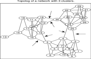
Figure 7: A sample of topology with three clusters: cluster $1$ contains nodes $1$–$10$, cluster $2$ nodes $11$–$20$ and cluster $3$ nodes $21$–$30$.

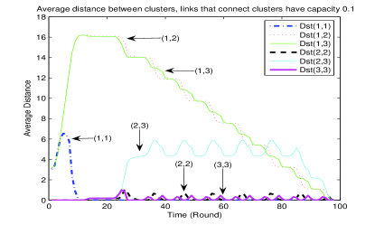
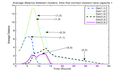
Figure 8: Simulation results for the topology in Figure 7, with bottleneck link capacity values equal to $0.1$ (left) and $1$ (right).

VI-D Simulation Results

For our simulation results we will start from randomly generated topologies similar to Figure 7, that consists of $30$ nodes connected into three distinct clusters. The source is node $1$, and belongs in the first cluster. The bottleneck links are indicated with arrows (and thus indicate the underlying physical link structure). Our first set of simulation results depicted in Figure 8 show that the subspaces within each cluster are very similar, while the subspaces across clusters are significantly different, where we use the distance measure $D_{S}(\cdot,\cdot)$ defined in (2). These results indicate for example that knowledge of these subspaces will allow the registrat to accurately detect and break clusters (Algorithm 3).

Our second set of simulation results considers again topologies with three clusters: cluster $1$ has $15$ nodes and contains the source, cluster $2$ has also $15$ nodes, while the number of nodes in cluster $3$ increases from $15$ to $250$. During the simulations we assume that the registrat keeps the nodes’ degree between $2$ and $5$, with an average degree of $3.5$. All edges correspond to unit capacity links.

We compare the performance of the three proposed algorithms in §VI-C with random rewiring. We implemented these algorithms as follows. For random rewiring, every time a node receives a packet it changes one of its neighbors with probability $p=\frac{8}{500}$. For Algorithm 1, we use a parameter of $k=10$, and check whether the non-innovative packets received exceed this value every four received packets. For Algorithm 2, every node checks each received subspaces every four received packets using the threshold value $\mathcal{T}=1$. Finally for Algorithm $3$, we assume that nodes use the same criterion as in Algorithm 2 to decide whether they form part of a cluster, again with $\mathcal{T}=1$. Dissatisfied nodes send their observed subspaces to the registrat. The registrat assigns nodes $u$ and $v$ in the same cluster if $d_{S}(\Pi_{u},\Pi_{v})\leq 7$.

Table I compares all algorithms with respect to the average collection time, defined as the difference between the time a peer receives the first packet and the time it can decode all packets, and averaged over all peers. All algorithms perform similarly, indicating that all algorithms result in breaking the clusters. It is important to note that the average collection time is in terms of number of exchanges needed and does not account for the delays incurred due to rewiring. We compare the number of such rewirings needed next.

Figure 9 plots the average number of rewirings each algorithm employs. Random rewiring incurs a number of rewirings proportional to the number of P2P nodes, and independently from the underlying network topology. Our proposed algorithms on the other hand, adapt to the existence and size of clusters. Algorithm $3$ leads to the smallest number of rewirings. Algorithm $2$ leads to a larger number of rewirings, partly due to that the new neighbors are chosen randomly and not in a manner that necessarily breaks the clusters. The behavior of algorithm $1$ is interesting. This algorithm rewires any node that has received more than $k$ non-innovative packets. Consider cluster $3$, whose size we increase for the simulations. If $k$ is small with respect to the cluster size, then a large number of nodes will collect close to $k$ non-innovative packets; thus a large number of nodes will ask for rewirings. Moreover, even after rewirings that break the cluster occur, some nodes will still collect linearly dependent information and ask for additional rewirings. As cluster $3$ increases in size, the information disseminates more slowly within the cluster. Nodes in the border, close to the bottleneck links, will now be the ones to first ask for rewirings, long before other nodes in the network collect a large number of non-innovative packets. Thus once the clusters are broken, no new rewirings will be requested. This desirable behavior of Algorithm $1$ manifests itself for large clusters; for small clusters, such as cluster $2$, the second algorithm for example achieves a better performance using less reconnections.

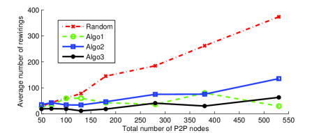
Figure 9: Average number of rewirings, for a topology with three clusters: cluster $1$ has $15$ nodes, cluster $2$ has $15$ nodes, while the number of nodes in cluster $3$ increases from $20$ to $250$ as described in Table I.

TABLE I: Average Collection Time

Topology	Random	Algo 1	Algo 2	Algo 3
$15$–$15$–$20$	$20.98$	$22.14$	$20.57$	$20.39$
$15$–$15$–$40$	$18.72$	$21.13$	$19.36$	$19.47$
$15$–$15$–$70$	$18.88$	$21.54$	$18.97$	$19.54$
$15$–$15$–$100$	$18.6$	$21.48$	$18.91$	$21.42$
$15$–$15$–$150$	$19.56$	$20.85$	$19.96$	$20.18$
$15$–$15$–$250$	$18.79$	$19.8$	$19.18$	$18.99$

VII Conclusions and Discussion

In this work we explored the properties of subspaces each node collects in networks that employ randomized network coding and found that there exists an intricate relationship between the structure of the network and these properties. This observation led us to utilize these relationships in several different applications. As the first application, we studied the conditions under which we can passively infer the network topology during content distribution. We showed that these conditions are not very restrictive and hold for a general class of information dissemination protocols. As our second application, we focused on locating Byzantine attackers in the network. We studied and formulated this problem and found that for the single adversary we can identify the adversary within an uncertainty of two nodes. For the case of multiple adversaries, we discussed a number of algorithms and conditions under which we can guarantee identifiability. For our last application, we investigated the relation between the bottlenecks in a logical network and the subspaces received at a specific network node. We leveraged our observations to propose decentralized peer-initiated algorithms for rewiring in P2P systems to avoid clustering in a cost-efficient manner, and evaluated our algorithms through simulations results.

The applications studied in this paper demonstrate advantages of using randomized network coding for network management and control, that are additional to throughput benefits. These are just a few examples and we believe that there exist a lot more applications where we can use the subspace properties developed in this work. We hope that these properties will become part of a toolbox that can be used to develop applications for systems that employ network coding techniques.

Appendix A Proofs

Proof:

First, let us fix a basis for $\Pi_{S}$. Then choosing $m$ vector uniformly at random from $\Pi_{S}$ is equivalent to choose an $m\times n$ matrix $\boldsymbol{A}$ uniformly at random from $\mathbb{F}_{q}$ and construct $\Pi=\left\langle\boldsymbol{A}\right\rangle$ with respect to this fixed basis.

It is well known (e.g., see [35]) that the number of different $m\times n$ matrices $\boldsymbol{A}$ with rank $0\leq k\leq\min[m,n]$ over $\mathbb{F}_{q}$ is equal to

$$N_{m,n}(k)\triangleq q^{(m+n-k)k}\prod_{i=0}^{k-1}\frac{(1-q^{i-n})(1-q^{i-m})}{(1-q^{i-k})}.$$

So we can write

$${\mathbb{P}\left[\dim(\Pi)=k\right]} =\frac{N_{m,n}(k)}{q^{mn}}.$$

Then using the Taylor series $\frac{1}{1-\epsilon}=1+\epsilon+\epsilon^{2}+\cdots$ for $|\epsilon|<1$, choosing $\epsilon=q^{-1}$, we can write

$$\Pr[\dim(\Pi)=k]=q^{-(m-k)(n-k)}[1-O(q^{-1})].$$

By setting $k=\min[m,n]$ we are done. ∎

Proof:

The probability that all $m$ vectors are in the intersection is

$${\mathbb{P}\left[\Pi_{1}^{\prime}\subset\Pi_{2}\right]} = \left(\frac{q^{d_{12}}}{q^{d_{1}}}\right)^{m}=q^{(d_{12}-d_{1})m},$$

which is of order $O\left(q^{-m}\right)$ provided that $\Pi_{1}\nsubseteq\Pi_{2}$ , i.e., $d_{12}<d_{1}$. ∎

Proof:

Let $\boldsymbol{v}_{1},\ldots,\boldsymbol{v}_{m}$ be the vectors chosen randomly from $\Pi_{S}$ to construct $\Pi$, namely, we have $\Pi=\left\langle\boldsymbol{v}_{1},\dots,\boldsymbol{v}_{m}\right\rangle$. Then construct the sequence of subspaces $\Pi(i)$, $i=0,\ldots,m$, as follows. First, set $\Pi(0)\triangleq\Pi_{k}$ and then define $\Pi(i)$ for $i\neq 0$ recursively, $\Pi(i)=\Pi(i-1)+\left\langle\boldsymbol{v}_{i}\right\rangle$. We also define $d(i)\triangleq\dim(\Pi(i))$, $i=0,\ldots,m$. From Lemma 2, by choosing $\Pi_{1}=\Pi_{S}$, $\Pi_{2}=\Pi(i-1)$ and $m=1$ we deduce that $d(i)=d(i-1)+1$ with probability $1-O\left(q^{-1}\right)$, unless $d(i-1)=n$.

Now we consider two cases. First, if $m+k\leq n$ then we have $\dim(\Pi+\Pi_{k})=k+m$ or equivalently $\dim(\Pi\cap\Pi_{k})=0$ with high probability, i.e., $1-O\left(q^{-1}\right)$. Secondly, when $m+k>n$ we have $\dim(\Pi+\Pi_{k})=n$ with probability $1-O\left(q^{-1}\right)$. From Lemma 1 we have $\dim(\Pi)=\min[m,n]$ w.h.p. So we have $\dim(\Pi\cap\Pi_{k})=\dim(\Pi_{k})+\dim(\Pi)-\dim(\Pi_{k}\cup\Pi)=k+\min[m,n]-n$.

Combining these two cases we can write

$$\dim(\Pi\cap\Pi_{k})=(k+\min[m,n]-n)^{+},$$

w.h.p., which completes the proof. ∎

Proof:

Let us define $\Pi_{12}=\Pi_{1}\cap\Pi_{2}$, where $d_{12}=\dim(\Pi_{12})$. Using Lemma 3, and taking $\Pi_{S}=\Pi_{1}$ and $\Pi_{k}=\Pi_{12}$, we have

$$\dim(\hat{\Pi}_{1}\cap\Pi_{12})=\min\left[d_{12},(m_{1}-(d_{1}-d_{12}))^{+}\right],$$

with probability $1-O\left(q^{-1}\right)$. Now, we can write

$${\mathbb{P}\left[\hat{d}_{12}=\alpha\right]}=$$

$${\mathbb{P}\left[\hat{d}_{12}=\alpha|\dim(\hat{\Pi}_{1}\cap\Pi_{12})=\beta\right]}{\mathbb{P}\left[\dim(\hat{\Pi}_{1}\cap\Pi_{12})=\beta\right]}$$

$$+{\mathbb{P}\left[\hat{d}_{12}=\alpha|\dim(\hat{\Pi}_{1}\cap\Pi_{12})\neq\beta\right]}{\mathbb{P}\left[\dim(\hat{\Pi}_{1}\cap\Pi_{12})\neq\beta\right]},$$

where $\hat{d}_{12}=\dim(\hat{\Pi}_{1}\cap\hat{\Pi}_{2})$. Substituting $\beta=\min\left[d_{12},(m_{1}-(d_{1}-d_{12}))^{+}\right]$ we obtain

$${\mathbb{P}\left[\hat{d}_{12}=\alpha\right]}=$$

$${\mathbb{P}\left[\hat{d}_{12}=\alpha|\dim(\hat{\Pi}_{1}\cap\Pi_{12})=\beta\right]}\left(1-O\left(q^{-1}\right)\right)+O\left(q^{-1}\right).$$

Selecting $\alpha$ properly and using Lemma 3 one more time, we get

$${\mathbb{P}\left[\hat{d}_{12}=\alpha\right]}=1-O\left(q^{-1}\right),$$

where $\alpha=\min[\beta,(m_{2}-(d_{2}-\beta))^{+}]$, which completes the proof. ∎

Proof:

To prove the theorem, it is sufficient to show that (5) is valid for one specific $i$ with high probability. This is sufficient because if $p_{i}$ is the probability that $\Pi$ is in general position with respect to each $\Pi_{i}$, $i=1,\ldots,r$, then the probability that $\Pi$ is in general position with the whole family is lower bounded by $1-\sum_{i=1}^{r}(1-p_{i})$.

Now by applying Lemma 3, we know that $p_{i}=1-O\left(q^{-1}\right)$ which completes the proof. ∎

Proof:

Here we assume that $n$ is very large. Then in Corollary 3 we will derive a sufficient condition on the largeness of $n$.

Let $v$ be the node that has the longest path to the source $S$. Because of Definition 1 we can write $T_{s}\leq\tau_{v}-1$. Then we may upper bound $\tau_{v}$ as follows

$$\tau_{v}\leq 2+\max_{u\in P(v)}\tau_{u},$$

where $P(v)$ is the set of parents of $v$. Now we can repeat the above argument until we reach the source $S$. So finally we have

$$\tau_{v}\leq 2D(G),$$

which leads to the lemma’s assertion. ∎

Proof:

Let us write

$$\dim( \pi_{u}(1)\cap\Pi_{v}(j))$$

$$\stackrel{{\scriptstyle(a)}}{{=}}\dim\left(\pi_{u}(1)\cap(\Pi_{v}(j)\cap\Pi(0))\right)$$

$$\stackrel{{\scriptstyle(b)}}{{=}}\dim(\pi_{u}(1)\cap\pi_{v}(1))$$

$$\stackrel{{\scriptstyle(c)}}{{=}}\min[d_{0},(k_{u}(1)+k_{v}(1)-d_{0})^{+},k_{u}(1),k_{v}(1)]$$

$$=(k_{u}(1)+k_{v}(1)-d_{0})^{+}$$

$$<k_{u}(1),$$

where $(a)$ follows because $\pi_{u}(1)\subseteq\Pi(0)$ and $(c)$ is a result of Corollary 2. So $\forall j\in\{1,\ldots,t\}$ we have $\pi_{u}(1)\nsubseteq\Pi_{v}(j)$ which results in $\Pi_{u}(i)\nsubseteq\Pi_{v}(j)$, $\forall i,j\in\{1,\ldots,t\}$. By symmetry, we have the second assertion of the lemma, namely, $\Pi_{v}(j)\nsubseteq\Pi_{u}(i)$, $\forall i,j\in\{1,\ldots,t\}$.

Now, it only remains to check $(b)$. We will prove this by induction. Obviously, $\Pi(0)\cap\Pi_{v}(1)=\pi_{v}(1)$. Suppose that we have $\Pi(0)\cap\Pi_{v}(k)=\pi_{v}(1)$ where $k<t$ then we show that it also holds for $k+1$.

We know that $\pi_{v}(1)\subseteq\Pi(0)\cap\Pi_{v}(k+1)$. To show that $\Pi(0)\cap\Pi_{v}(k+1)\subseteq\pi_{v}(1)$ we proceed as follows. Let $w\in\Pi(0)\cap\Pi_{v}(k+1)$ then $w\in\Pi(0)$ and $w\in\Pi_{v}(k+1)=\sum_{i=1}^{k+1}\pi_{v}(i)$. We may decompose $w$ as $w=\sum_{i=1}^{k+1}w_{i}$ where $w_{i}\in\pi_{v}(i)$. Then we notice that $w_{k+1}=w-\sum_{i=1}^{k}w_{i}\in\Pi(k-1)$ and $\Pi(k-1)\cap\pi_{v}(k+1)=\emptyset$ w.h.p. (by Lemma 3). So we conclude that $w_{k+1}=0$ which means $w\in\Pi_{v}(k)$. This shows that $w\in\Pi(0)\cap\Pi_{v}(k)$ where by induction assumption we have $w\in\pi_{v}(1)$ and we are done. ∎

Proof:

Because we have $\Pi_{u}(0)\nsubseteq\Pi_{v}(j)$ then by Lemma 2 we have $\pi_{a}(1)\nsubseteq\Pi_{v}(j)$ w.h.p. So as a result we have $\Pi_{a}(i)\nsubseteq\Pi_{v}(j-1)$ $\forall i,j\in\{1,\ldots,t\}$. Because $\Pi_{b}(j)\subseteq\Pi_{v}(j-1)$ we conclude that $\Pi_{a}(i)\nsubseteq\Pi_{b}(j)$ $\forall i,j\in\{1,\ldots,t\}$ w.h.p. By symmetry, we also deduce the other part of the corollary. ∎

Appendix B Algebraic Model for Synchronous Networks

In this appendix we employ an algebraic approach to analyze the dissemination protocol given in Algorithm II. This approach is similar to [15] and [1], but differs in that we introduce memory into the coding process.

We introduce memory as follows. Suppose we are interested in finding the transfer function between the source and an arbitrary node $v$. Let $\boldsymbol{X}$ be a $n\times\ell$ matrix with rows the $n$ packets (vectors) that the source wants to transmit to the receivers. We assume that $\dim(\left\langle\boldsymbol{X}\right\rangle)=n$. Let $\boldsymbol{Y}(t)\in\mathbb{F}_{q}^{\xi\times\ell}$ be a matrix with rows the packets that pass through the $\xi$ edges of the network at time $t$. Let $\boldsymbol{Z}_{v}(t)$ be the set of packets that node $v$ receives. Similarly to [15], we will write state-space equations that involve these vectors; however, we will ensure that, at each time $t$, coding at each node occurs across all the packets that the node has received before time $t$.

In each timeslot $t$, the source injects $|\operatorname{Out}(S)|$ packets into the network that are random linear combinations of the original source packets $\boldsymbol{X}$. These linear combinations can be captured as $\boldsymbol{M}(t)\boldsymbol{X}$, where $\boldsymbol{M}(t)\in\mathbb{F}_{q}^{|\operatorname{Out}(S)|\times n}$ is a random matrix. Intermediate network nodes will transmit packets on their outgoing edges depending on the network connectivity, and the state of the dissemination protocol.

The network connectivity can be captured by the $\xi\times\xi$ adjacency matrix $\mathcal{F}$ of the labeled line graph of the graph $G$, defined as follows

$$\mathcal{F}_{ij}\triangleq\left\{\begin{array}[]{ll}1&\operatorname{head}(e_{i})=\operatorname{tail}(e_{j}),\\ 0&\textrm{otherwise.}\end{array}\right.$$

To model random coding over a field $\mathbb{F}_{q}$, we consider a sequence of random matrices $\boldsymbol{F}_{1}^{(t)},\ldots,\boldsymbol{F}_{t-1}^{(t)}$ which conform to $\mathcal{F}$. That is, the entries of these matrices have for $i\neq j$ $(\boldsymbol{F}_{k}^{(t)})_{ij}=0$ wherever $\mathcal{F}_{ij}=0$ and have random numbers from $\mathbb{F}_{q}$ in all other places.

The dissemination protocol dictates when a node can start transmitting packets, according to its waiting time (equivalently, when the outgoing edges of the node will have packets send through them). To capture this, we will use the step function $u(t)$,

$$u(t)\triangleq\left\{\begin{array}[]{l}1\quad t\geq 0,\\ 0\quad\textrm{otherwise},\end{array}\right.$$

and define the $\xi\times\xi$ diagonal matrix $\boldsymbol{U}(t)$ as,

$$\forall i\in E:\quad\boldsymbol{U}_{ii}(t)\triangleq u\left(t-\tau_{\operatorname{tail}(i)}-1\right),$$

where $\tau_{v}$ is the waiting time for node $v$. In this section we assume that the waiting times may have arbitrary values and we do not restrict them according to Definition 1.

Using the above definitions, the set of packets (vectors) that each node $v$ receives in every time instant $t>0$ can be written as follows

$$\left\{\begin{array}[]{l}\boldsymbol{Y}(t)=\boldsymbol{U}(t)\left(\boldsymbol{A}\boldsymbol{M}(t)\boldsymbol{X}+\sum_{i=1}^{t-1}\boldsymbol{F}_{i}^{(t)}\boldsymbol{Y}(t-i)\right),\\ \\ \boldsymbol{Z}_{v}(t)=\boldsymbol{B}_{v}\boldsymbol{Y}(t),\end{array}\right.$$ (11)

where $\boldsymbol{Y}(0)=\boldsymbol{0}$. In the above, $\boldsymbol{A}\in\mathbb{F}_{q}^{\xi\times|\operatorname{Out}(S)|}$ is a matrix which represents the connection of node $S$ to the rest of the network. In the same way matrix $\boldsymbol{B}_{v}\in\mathbb{F}_{q}^{|\operatorname{In}(v)|\times\xi}$ defines the connection of node $v$ to the set of edges in the network.

It is worth noting that although (11) is written for the packets transmitted on each edge, we can write the same set of equations for the coding vectors.

Suppose we are interested in finding the output of such a system at some time instant $T$. We can rewrite the above equations by defining new matrices as follows. We can collect the source random operations as

$$\boldsymbol{M}_{T}\triangleq\left[\begin{array}[]{c}\boldsymbol{M}(1)\\ \vdots\\ \boldsymbol{M}(T)\end{array}\right]\in\mathbb{F}_{q}^{T|\operatorname{Out}(S)|\times n}.$$

For the states of system we define

$$\boldsymbol{Y}_{T}\triangleq\left[\begin{array}[]{c}\boldsymbol{Y}(1)\\ \vdots\\ \boldsymbol{Y}(T)\end{array}\right]\in\mathbb{F}_{q}^{\xi T\times\ell}.$$

We also define a new set of matrices which represent the input-output relation. Using matrix $\boldsymbol{A}$ we define the following matrix

$$\boldsymbol{A}_{T}\triangleq\boldsymbol{I}_{T}\otimes\boldsymbol{A}=\left[\begin{array}[]{ccc}\boldsymbol{A}&&\\ &\ddots&\\ &&\boldsymbol{A}\end{array}\right]\in\mathbb{F}_{q}^{\xi T\times T|\operatorname{Out}(S)|}.$$

For the connection of node $v$ we define

$$\boldsymbol{B}_{v}(T)\triangleq\left[\begin{array}[]{cc}\boldsymbol{0}_{|\operatorname{In}(v)|\times(T-1)\xi}&\boldsymbol{B}_{v}\\ \end{array}\right]\in\mathbb{F}_{q}^{|\operatorname{In}(v)|\times\xi T}.$$

We define matrix $\boldsymbol{F}_{T}$ which represent how the states are related to each other

$$\boldsymbol{F}_{T}\triangleq\left[\begin{array}[]{ccccc}\boldsymbol{0}&\boldsymbol{0}&\boldsymbol{0}&\boldsymbol{0}&\cdots\\ \boldsymbol{F}_{1}^{(2)}&\boldsymbol{0}&\boldsymbol{0}&\boldsymbol{0}&\cdots\\ \boldsymbol{F}_{2}^{(3)}&\boldsymbol{F}_{1}^{(3)}&\boldsymbol{0}&\boldsymbol{0}&\cdots\\ \boldsymbol{F}_{3}^{(4)}&\boldsymbol{F}_{2}^{(4)}&\boldsymbol{F}_{1}^{(4)}&\boldsymbol{0}&\cdots\\ \vdots&\vdots&\vdots&\vdots&\ddots\end{array}\right]\in\mathbb{F}_{q}^{\xi T\times\xi T}.$$

Finally, we use matrix $\boldsymbol{U}_{T}$ that captures the time when transmissions start for each edge

$$\boldsymbol{U}_{T}\triangleq\left[\begin{array}[]{ccc}\boldsymbol{U}(1)&&\\ &\ddots&\\ &&\boldsymbol{U}(T)\end{array}\right]\in\mathbb{F}_{q}^{\xi T\times\xi T}.$$

Using the above definitions, we can rewrite (11) as follows

$$\left\{\begin{array}[]{l}\boldsymbol{Y}_{T}=\boldsymbol{U}_{T}\left(\boldsymbol{A}_{T}\boldsymbol{M}_{T}\boldsymbol{X}+\boldsymbol{F}_{T}\boldsymbol{Y}_{T}\right),\\ \\ \boldsymbol{Z}_{v}(T)=\boldsymbol{B}_{v}(T)\boldsymbol{Y}_{T}.\end{array}\right.$$

This equation can be solved to find the input-output transfer matrix at time $T$ which results in

$$\boldsymbol{Z}_{v}(T)=\underbrace{\left[\boldsymbol{B}_{v}(T)(\boldsymbol{I}-\boldsymbol{U}_{T}\boldsymbol{F}_{T})^{-1}\boldsymbol{U}_{T}\boldsymbol{A}_{T}\boldsymbol{M}_{T}\right]}_{\boldsymbol{H}_{Sv}(T)}\boldsymbol{X},$$ (12)

where $\boldsymbol{H}_{Sv}(T)\in\mathbb{F}_{q}^{|\operatorname{In}(v)|\times n}$. From the definition of matrix $\boldsymbol{F}_{T}$, we know that it is a “strictly lower triangular matrix” which means $\boldsymbol{F}_{T}$ is nilpotent and we have $\boldsymbol{F}_{T}^{T}=0$. The same applies for the matrix $\boldsymbol{U}_{T}\boldsymbol{F}_{T}$, namely we have $(\boldsymbol{U}_{T}\boldsymbol{F}_{T})^{T}=0$. So the matrix $(\boldsymbol{I}-\boldsymbol{U}_{T}\boldsymbol{F}_{T})^{-1}$ has an inverse which is equal to

$$(\boldsymbol{I}-\boldsymbol{U}_{T}\boldsymbol{F}_{T})^{-1}=\left(\boldsymbol{I}+\cdots+(\boldsymbol{U}_{T}\boldsymbol{F}_{T})^{T-1}\right).$$

Finally, note that if the nodes do not wait before starting the transmission ($\tau_{v}=0:\ \forall v\in V$), then we will have $\boldsymbol{U}_{T}=\boldsymbol{I}_{\xi T\times\xi T}$.

B-A Proof of Theorem 2

For simplicity, in the following proof, we assume that each edge of the network has capacity $1$. Edges with capacity more than $1$ can be modeled by replacing them with multiple edges of unit capacity.

From (12) the transfer matrix from $S$ to $v$ at time $T$ is equal to $\boldsymbol{H}_{Sv}(T)$. Knowing that the min-cut of node $v$ is $c_{v}$, we choose a set of $c_{v}$ incoming edges to $v$ such that there exist $c_{v}$ edge disjoint paths from $S$ to $v$ and find the input-output transfer matrix just for this set of edges. Then we can write

$$\boldsymbol{\hat{H}}_{Sv}(T) =\boldsymbol{\hat{B}}_{v}(T)(\boldsymbol{I}-\boldsymbol{U}_{T}\boldsymbol{F}_{T})^{-1}\boldsymbol{U}_{T}\boldsymbol{A}_{T}\boldsymbol{M}_{T}$$ (13)

$$=\boldsymbol{\hat{B}}_{v}(T)\left(\boldsymbol{I}+\cdots+(\boldsymbol{U}_{T}\boldsymbol{F}_{T})^{T-1}\right)\boldsymbol{U}_{T}\boldsymbol{A}_{T}\boldsymbol{M}_{T},$$

where $\boldsymbol{\hat{H}}_{Sv}(T)\in\mathbb{F}_{q}^{c_{v}\times n}$ and $\boldsymbol{\hat{B}}_{v}(T)\in\mathbb{F}_{q}^{c_{v}\times\xi T}$. Let $f_{ij}^{(t,k)}$ denote for the entries of $\boldsymbol{F}_{k}^{(t)}$ and $m_{ij}^{(t)}$ denote for the entries of $\boldsymbol{M}(t)$. Every node in the network performs random linear network coding so $m_{ij}^{(t)}$ and $f_{ij}^{(t,k)}$ (those that are not zero) are chosen uniformly at random from $\mathbb{F}_{q}$.

From (13) we know that each entry of ${\boldsymbol{\hat{H}}}_{Sv}(T)$ is a polynomial of degree at most $T$ in variables $m_{ij}^{(t)}$ and $f_{ij}^{(t,k)}$. For $T>t_{0}(v)$ where $t_{0}(v)\triangleq\max_{i\in P(v)}\tau_{i}$, we know that there exists a trivial solution for variables $m_{ij}^{(t)}$ and $f_{ij}^{(t,k)}$ (which simply routes $c_{v}$ packets from $S$ to $v$ through the $c_{v}$ edge disjoint paths) that results in

$$\boldsymbol{\hat{H}}_{Sv}(T)=\left[\begin{array}[]{cc}\boldsymbol{I}_{c_{v}}&\boldsymbol{0}_{c_{v}\times(n-c_{v})}\end{array}\right].$$ (14)

Note that by changing the routing solution (in fact by changing the variables $m_{ij}^{(t)}$ properly) we could change the place of identity matrix in (14) arbitrarily. We conclude that the determinant of every $c_{v}\times c_{v}$ submatrix of $\boldsymbol{\hat{H}}_{Sv}(T)$ (which is a polynomial of degree at most $c_{v}T$ in variables $m_{ij}^{(t)}$ and $f_{ij}^{(t,k)}$) is not identical to zero. So by using the Schwartz-Zippel lemma [36] we can upper bound the probability that $\boldsymbol{\hat{H}}_{Sv}(T)$ is not full rank if the variables $m_{ij}^{(t)}$ and $f_{ij}^{(t,k)}$ are chosen uniformly at random as follows

$${\mathbb{P}\left[\operatorname{rank}{\boldsymbol{\hat{H}}_{Sv}(T)}<c_{v}\right]}<\frac{c_{v}T}{q}.$$

We can apply the same argument for $k<\frac{n}{c_{v}}$ consecutive timeslots to show that

$${\mathbb{P}\left[\operatorname{rank}{\boldsymbol{\hat{H}}_{Sv}(T:T+k-1)}<kc_{v}\right]}<\frac{kc_{v}(T+k)}{q},$$

where

$$\boldsymbol{\hat{H}}_{Sv}(T:T+k-1)\triangleq\left[\begin{array}[]{c}\boldsymbol{\hat{H}}_{Sv}(T)\\ \vdots\\ \boldsymbol{\hat{H}}_{Sv}(T+k-1)\end{array}\right].$$

Now let us define the event $\mathcal{A}_{k}(v)$ as follows

$$\mathcal{A}_{k}(v):\ \operatorname{rank}{\boldsymbol{\hat{H}}_{Sv}(T:T+k-1)}=kc_{v}.$$

Then we can write

$${\mathbb{P}\left[\cap_{v\in V}\mathcal{A}_{k}(v)\right]} =1-{\mathbb{P}\left[\cup_{v\in V}\mathcal{A}_{k}^{\complement}(v)\right]}$$

$$\geq 1-\sum_{v\in V}{\mathbb{P}\left[\mathcal{A}_{k}^{\complement}(v)\right]}$$

$$\geq 1-\frac{k(T+k)}{q}\sum_{v\in V}c_{v},$$

where $T>t_{0}$ and $t_{0}\triangleq\max_{v\in V}t_{0}(v)$.

This means that assuming $q$ is large enough we are sure that with high probability each node $v$ receives $c_{v}$ innovative packets per time slot for $t>t_{0}$.

References

- [1] T. Ho, R. Koetter, M. Medard, M. Effros, J. Shi, and D. Karger, “A random linear network coding approach to multicast,” IEEE Transactions on Information Theory, vol. 52, pp. 4413–4430, Oct. 2006.
- [2] P. A. Chou, Y. Wu, and K. Jain, “Practical network coding,” Allerton, Monticello, IL, Oct. 2003.
- [3] C. Gkantsidis and P. Rodriguez, “Network coding for large scale content distribution,” in the Proceedings of IEEE INFOCOM, Mar. 2005.
- [4] C. Gkantsidis, J. Miller, and P. Rodriguez, “Comprehensive view of a live network coding P2P system,” ACM SIGCOMM/USENIX IMC, 2006.
- [5] Wei Li-shuang, Song Wei, Hu Wen-bin and Hu Zheng-bing, “Using network coding makes P2P content sharing scalable”, 2nd International Workshop on Database Technology and Applications (DBTA), 2010.
- [6] Xi Wei and Dong-Yang Long, “P2P Content-Propagation Mechanism Tailored by Network Coding”, International Symposium on Computer Network and Multimedia Technology, CNMT 2009.
- [7] X. Zhang and B. Li, “On the market power of network coding in P2P content distribution systems,” INFOCOM, pp. 334–342, Apr. 2009.
- [8] D. S. Lun, N. Ratnakar, M. Medard, R. Koetter, D. R. Karger, T. Ho, E. Ahmed, and F. Zhao, “Minimum-cost multicast over coded packet networks”, IEEE Trans. Inform. Theory, vol. 52, no. 6, pp. 2608–2623, Jun. 2006.
- [9] C. Fragouli, J. Widmer and J. Y. Le Boudec, “A network coding approach to energy efficient broadcasting: from theory to practice,” Proceedings INFOCOM, 25th IEEE International Conference on Computer Communications, Barcelona, pp. 1–11, Apr. 2006.
- [10] M. Jafari Siavoshani, C. Fragouli, and S. Diggavi, “Subspace properties of randomized network coding,” IEEE Information Theory Workshop, pp. 17–21, Bergen, Norway, Jul. 2007.
- [11] M. Jafari Siavoshani, C. Fragouli, S Diggavi, and C. Gkantsidis, “Bottleneck discovery and overlay management in network coded peer-to-peer systems,” ACM SIGCOMM Workshop on Internet Network Management, Kyoto, Japan, Aug. 2007.
- [12] M. Jafari Siavoshani, C. Fragouli, S. Diggavi, “On locating byzantine attackers,” Network Coding Workshop, Jan. 2008.
- [13] R. Ahlswede, N. Cai, S-Y. R. Li, and R. W. Yeung, “Network information flow,” IEEE Transactions on Information Theory, vol. 46, pp. 1204–1216, Jul. 2000.
- [14] S.-Y. R. Li, R. W. Yeung, and N. Cai., “Linear network coding,” IEEE Transactions on Information Theory, vol. 49, pp. 371–381, 2003.
- [15] R. Koetter, M. Medard, “An algebraic approach to network coding,” Transactions on Networking, Oct. 2003.
- [16] T. Ho, R. Koetter, M. Medard, D. Karger and M. Effros, “The benefits of coding over routing in a randomized setting,” IEEE International Symposium on Information Theory, 2003.
- [17] R. Koetter and F. Kschischang, “Coding for errors and erasures in random network coding,” IEEE Transactions on Information Theory, vol. 54, no. 8, pp. 3579–3591, Aug. 2008.
- [18] S. Jaggi, M. Langberg, S. Katti, T. Ho, D. Katabi, and M. Medard, “Resilient network coding in the presence of byzantine adversaries,” in the Proceedings of IEEE INFOCOM, pp. 616–624, 2007.
- [19] T. Ho, B. Leong, R. Koetter, M. Medard, M. Effros, and D. Karger, “Byzantine modification detection in multicast networks using randomized network coding,” IEEE International Symposium of Information Theory, Jun. 2004.
- [20] R. W. Yeung and N. Cai, “Network error correction, i: basic concepts and upper bounds,” Communication and Information System, vol. 6, pp. 19–35, 2006.
- [21] N. Cai and R. W. Yeung, “Network error correction, ii: lower bounds,” Communication and Information System, vol. 6, pp. 37–54, 2006.
- [22] Z. Zhang, “Network error correction coding in packetized networks,” IEEE Information Theory Workshop, Oct. 2006.
- [23] D. Silva and F. R. Kschischang, “Universal secure network coding via rank-metric codes,” IEEE Transactions on Information Theory, vol. 57, no. 2, pp. 1124–1135, Feb. 2011.
- [24] E. Kehdi and B. Li, “Null keys: Limiting malicious attacks via null space properties of network coding,” in the Proceedings of IEEE INFOCOM, pp. 19–25, Brazil, Apr. 2009.
- [25] “RON: Resilient Overlay Networks,” available online at http://nms.csail.mit.edu/ron.
- [26] C. Fragouli and A. Markopoulou, “A network coding approach to overlay network monitoring,” Allerton, Oct. 2005.
- [27] C. Fragouli, A. Markopoulou, and S. Diggavi, “Active topology inference using network coding,” Allerton, Oct. 2006.
- [28] T. Ho, B. Leong, Y. Chang, Y. Wen, and R. Koetter, “Network monitoring in multicast networks using network coding,” IEEE International Symposium on Information Theory, Jun. 2005.
- [29] G. Sharma, S. Jaggi, and B. K. Dey, “Network tomography via network coding,” in Proceeding of ITA Workshop, UCSD, 2007.
- [30] M. Jafari Siavoshani, C. Fragouli, and S. Diggavi, “Noncoherent multisource network coding,” IEEE International Symposium on Information Theory, Toronto, Canada, pp. 817–821, Jul. 2008.
- [31] D. Silva, F. R. Kschischang, and R. Koetter, “Communication over finite-field matrix channels,” IEEE Transactions on Information Theory, vol. 56, iss. 3, pp. 1296–1305, Mar. 2010.
- [32] M. Jafari Siavoshani, S. Mohajer, C. Fragouli, S N. Diggavi, “On the capacity of non-coherent network coding,” IEEE Transactions on Information Theory, to be appeared in Feb. 2011.
- [33] L. Babai and P. Frankl, “Linear algebra methods in combinatorics,” preliminary version, University of Chicago.
- [34] A. Al-Hamra, A. Legout, and C. Barakat, “Understanding the properties of the BitTorrent overlay,” INRIA Technical Report, available online at http://arxiv.org/pdf/0707.1820, Sophia Antipolis, France.
- [35] D. Laksov and A. Thorup, “Counting matrices with coordinates in finite fields and of fixed rank,” Mathematica Scandinavica, vol. 74, pp. 19–33, 1994.
- [36] R. Motwani and P. Raghavan, “Randomized Algorithms,” Cambridge University Press, 2000.