Nonequilibrium work statistics of an Aharonov-Bohm flux

Abstract

We investigate the statistics of work performed on a noninteracting electron gas confined into a ring as a threaded magnetic field is turned on. For an electron gas initially prepared in a grand canonical state it is demonstrated that the Jarzynski equality continues to hold in this case, with the free energy replaced by the grand potential. The work distribution displays a marked dependence on the temperature. While in the classical (high temperature) regime, the work probability density function follows a Gaussian distribution and the free energy difference entering the Jarzynski equality is null, the free energy difference is finite in the quantum regime, and the work probability distribution function becomes multimodal. We point out the dependence of the work statistics on the number of electrons composing the system.

I Introduction

One of the most fascinating electro-magnetic field effects is the modulation of quantum interference in multiply connected spatial regions due to electromagnetic fields. The Aharonov-Bohm (AB) effect is a well-known example where a localized magnetic field introduces the phase shift of a particle wavefunction and results in an interference pattern governed by the AB flux $\Phi_{AB}=\oint{\bf A}\cdot d{\bf l}$ ab . A similar effect, called the Aharonov-Casher (AC) effect occurs, when a neutral particle with a magnetic moment $\mu$ moves in an electric field ${\bf E}$ and acquires a phase shift amounting to the flux $\Phi_{AC}=\oint{\bf E}\times d{\bf l}\cdot\mbox{\boldmath{$\mu$}}/e$  ac ; ac2 ; ac3 . A dual effect was also pointed out for a neutral particle carrying an electric dipole moment moving in a magnetic field of the appropriate configuration dualac . In the mentioned examples, electromagnetic fields influence the wave function and also the energy spectrum of a particle moving in a multiply connected spatial region but do not exert any classical force.

Recently, scientists working in the field of non-equilibrium thermodynamics have drawn the attention to the fact that the work done by external forces on a driven system may be usefully employed to characterize their response properties. Jarzynski introduced the celebrated nonequilibrium work relation that links the free energy difference ($\Delta F$) to the averaged exponentiated negative work Jarzynski ; Jarzynski2 :

$$\langle e^{-\beta w}\rangle=e^{-\beta\Delta F},$$ (1)

where $w$ is the work performed on a system by a time-dependent force determined by a prescribed protocol and $\langle\cdots\rangle$ denotes the average over many realizations of the forcing experiment. The equality was primarily derived for classical systems, which experiments and theories so far mainly refer to classical1 ; classical2 ; classical3 . Fluctuation theorems in presence of magnetic fields and other non-conservative forces were studied for classical systems in Ref. Pradhan . On the other hand, generalizations of Eq. (1) to quantum mechanical systems were discussed quantum1 ; quantum2 ; quantum2b ; quantum3 ; TLH ; TH ; THM ; DL ; ftopen ; Talkner08PRE78 ; Talkner09PRE79 , for recent reviews see EHM ; CHT . In quantum mechanics, the work is obtained by means of two energy measurements at the beginning and at the end of a given protocol. In the mentioned examples of quantum interference effects, the electromagnetic fields do work on a charged particle, or a magnetic or electric dipole in multiply connected domains not only caused by the classical forces exerted on the particle but also by the shifts of the energy spectrum pc ; pc2 ; pc3 .

The main purpose of this work is to investigate the statistics of the work done by an Aharonov-Bohm flux for quantum charged particles moving along a one-dimensional ring representing the simplest possible multiply connected domain. We consider not only the single-particle case but also many-particle systems by generalizing the fluctuation theorem for a grand canonical initial state. Especially we focus on fermionic systems in a ring-configuration (see Fig. 1). Their equilibrium properties were discussed in terms of persistent currents decades ago pc ; pc2 ; pc3 ; loss . Recent measurement using nano-cantilevers to detect changes in the magnetic field produced by the current has achieved high accuracy and prompted a renewed interest in this topic pcexp . It is noteworthy that the focus of our study is laid upon the nonequilibrium nature of the system, revealed in the statistics of work done by the magnetic flux. By obtaining an analytic expression of the characteristic function of work, we examine the quantum and classical nature of the resulting distributions and study their dependence on both temperature and particle number.

The paper is organized as follows: Sec. II is devoted to the introduction of the system of interest. In Sec.III, we obtain the probability distribution for a single-particle case. We then consider a grand canonical initial state of many-particle systems, and present the results in Sec.IV. Summary and conclusion are drawn in Sec.V.

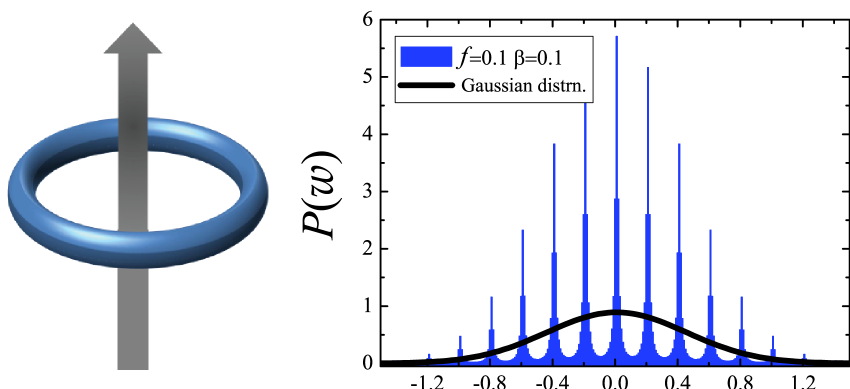
Figure 1: (Color online)  The left panel gives a schematic picture of a ring with a threading flux, and the right panel displays the work distribution consisting of a series of peaks for a single particle moving along the ring upon a sudden switch of the dimensionless flux $f=\Phi/\Phi_{0}$ from $f=0$ to $f=0.1$. The thick solid line represents the Gaussian approximation of the work distribution, Eq. (8), for the same parameter values.

II The system

We consider $N$ spinless fermions moving along an infinitely thin ring of radius $R$ in presence of a magnetic flux. The corresponding Hamiltonian reads loss

$${\cal H}_{f}=\frac{\hbar^{2}}{2mR^{2}}\sum_{\ell=1}^{N}\left(\frac{\partial}{i\partial\theta_{\ell}}-f\right)^{2},$$ (2)

where $\theta_{\ell}$ is the angular coordinate of the $\ell$th particle, and $f=\Phi/\Phi_{0}$ is the total flux threading the ring, $\Phi$, in units of the flux quantum, $\Phi_{0}=hc/e$. The single particle energy eigenvalues are given by loss

$$E_{k}(f)=E_{0}(k-f)^{2},$$ (3)

where $E_{0}=\hbar^{2}/2mR^{2}$ characterizes the energy-level spacing, and the integer $k$ denotes the angular momentum quantum number.

For later consideration of a many-particle system, let us introduce the second quantized form of the Hamiltonian:

$${\cal H}_{f}=\sum_{k}E_{k}(f)c_{k}^{\dagger}c_{k}\equiv\sum_{k}E_{k}(f){\cal N}_{k},$$ (4)

where $c_{k}^{\dagger}~{}(c_{k})$ is the creation (annihilation) operator of an electron in the $k$th angular momentum (or energy) eigenstate, and the number operator ${\cal N}_{k}=c_{k}^{\dagger}c_{k}$ measures the particle number in the $k$-th state.

We will study the probability distribution function $P(w)$ of the work $w$ that is performed on the electrons in the time span $[0,\tau]$, by a magnetic flux $f(t)$ that varies in time. As a consequence, the Hamiltonian of the system becomes time-dependent. It will be denoted by ${\cal H}(t)\equiv{\cal H}_{f(t)}$. Here we restrict ourselves to the case of a sudden switch of the magnetic flux immediately after the time $t=0$ with

$$f(t)=\left\{\begin{array}[]{ll}0&\text{for}\;t\leq 0\\ f&\text{for}\;t>0\end{array}\right.\>.$$ (5)

Given this protocol, we will first calculate the work characteristic function (i.e., the Fourier transform of $P(w)$), which for a canonical initial state is given by the formula TLH ; TH ; THM ; DL :

$$G(u)=\int_{\infty}^{-\infty}dwe^{iuw}P(w)=\langle e^{iu{\cal H}_{H}(\tau)}e^{-iu{\cal H}(0)}\rangle_{\rho_{c}},$$ (6)

and then obtain $P(w)$ by inverse Fourier transformation. Here $\langle X\rangle_{\rho_{c}}=\mbox{Tr}X\rho_{c}$ and $\rho_{c}=e^{-\beta{\cal H}(0)}/{\cal Z}_{0}$ with the normalization ${\cal Z}_{0}$ being the canonical partition function. Further, ${\cal H}_{H}(t)$ denotes the Hamiltonian operator in the Heisenberg representation. Note that since $[{\cal H}(t),{\cal H}(s)]=0$ for any $t$ and $s$ in the time span, the Hamiltonians in the Schrödinger and Heisenberg picture coincide, i.e. ${\cal H}_{H}(\tau)={\cal H}(\tau)$.

III Single particle case

In the case of a single particle system, we obtain from Eqs. (2) and (6),

$$G(u)=e^{iuE_{0}f^{2}}\sum_{k}e^{2ikfE_{0}u}e^{-\beta E_{0}k^{2}}/{\cal Z}_{0}.$$ (7)

We rescale all variables with the dimension of an energy by the natural energy unit $E_{0}$ as ${\widetilde{u}}=E_{0}u$, ${\widetilde{w}}=w/E_{0}$, and ${\widetilde{\beta}}=\beta E_{0}$ (for notational simplicity, we drop the tilde in the following). Note that at high temperatures the system enters the classical regime. In this regime we can discard the discretness of $k$ and replace the summation by an integration, namely, $\sum_{k}\rightarrow(R/\hbar)\int_{-\infty}^{\infty}dp$ with the momentum defined by $p=\hbar k/R$. We thus obtain $G(u)\approx G_{c}(u)=e^{if^{2}u-f^{2}u^{2}/\beta}$, which leads to a Gaussian distribution of work reading

$$P_{c}(w)=\sqrt{\beta/(4\pi f^{2})}e^{-\beta(w-f^{2})^{2}/(4f^{2})}\>.$$ (8)

Note that for $u=i\beta$, $G_{c}(i\beta)=\langle e^{-\beta w}\rangle=1$. This conversion from discrete summation to integration is accurate only at sufficiently high temperatures ($\beta\ll 1$), or for a ring of sufficiently large radius. When we fully count the level discretness, the work distribution is expected to be a series of peaks, and the normal distribution would provide its envelop. This can be confirmed by evaluating $P_{c}(w)$ directly from Eq. (7) via an inverse Fourier transform:

$$P(w)=\sum_{k}{\cal W}_{k}\delta(w-2kf-f^{2})$$ (9)

where ${\cal W}_{k}=e^{-\beta k^{2}}/\sum_{k}e^{-\beta k^{2}}$ is the weight of the $k$th peak. The right panel of Fig. 1 displays the resulting distribution note . It is then a due course to investigate many-particle cases, where the effect of finite particle number comes into question.

IV Grand canonical initial state

In order to deal with many-particle systems, we extend the characteristic function of work to initial grand canonical states. Although not needed here, we allow for possible changes of particle numbers. This will lead to a generalization of the Jarzynski work theorem to grand canonical initial states. Only later we will specify to the case of strict particle number conservation.

In the grand canonical ensemble energy and particle number are fluctuating quantities. In order to determine their changes effected by a protocol a simultaneous measurement of energy and particle number must be performed at the beginning and at the end of the protocol, see Ref. TCH where the joint statistics of changes of two observables are discussed. Joint measurements necessitate that the particle number operator $\cal{N}$ commutes with both the initial and final Hamiltonian, i.e., $[{\cal N},{\cal H}(\tau)]=[{\cal N},{\cal H}(0)]=0$. Then joint eigenfunctions $|\Psi_{\nu,N}(0)\rangle$ and $|\Psi_{{\bar{\nu}},\bar{N}}(\tau)\rangle$ exist with corresponding pairs of eigenvalues $E_{\nu}$, $N$ and $E_{{\bar{\nu}}}$, $\bar{N}$, satisfying ${\cal H}(\tau)|\Psi_{{\bar{\nu}},\bar{N}}(\tau)\rangle=E_{{\bar{\nu}},\bar{N}}(\tau)|\Psi_{{\bar{\nu}},\bar{N}}(\tau)\rangle$ and ${\cal N}|\Psi_{{\bar{\nu}}.\bar{N}}(\tau)\rangle={\bar{N}}|\Psi_{{\bar{\nu}},\bar{N}}(\tau)\rangle$, as well as ${\cal H}(0)|\Psi_{\nu,N}(0)\rangle=E_{\nu}(0)|\Psi_{\nu,N}(0)\rangle$ and ${\cal N}|\Psi_{\nu,N}(0)\rangle=N|\Psi_{\nu,N}(0)\rangle$. The joint probability density function ${\cal P}(w,n)$ to observe the work $w$ and particle number change $n$ in a single realization of the protocol is given by

$${\cal P}(w,n)=\sum_{\nu,{\bar{\nu}}}\sum_{N,{\bar{N}}} \delta(w -E_{{\bar{\nu}}}(\tau)+E_{\nu}(0))\delta_{n,{\bar{N}}-N}$$

$$\times P(E_{{\bar{\nu}}}(\tau),{\bar{N}}|E_{\nu}(0),N)P^{(eq)}_{g}(E_{\nu}(0),N),$$

where $P^{(eq)}_{g}=e^{-\beta(E_{\nu}-\mu N)}/{\cal Q}_{0}$ is the joint probability of finding the energy $E_{\nu}(0)$ and particle number $N$ in the initial grand-canonical state; further, ${\cal Q}_{0}=\sum_{\epsilon_{\nu},N}e^{-\beta(E_{\nu}(0)-\mu N)}$ that is the grand-canonical partition function. The conditional probability $P(E_{{\bar{\nu}}}(\tau),{\bar{N}}|E_{\nu}(0),N)$ for finding the energy $E_{{\bar{\nu}}}(\tau)$ and particle number $\bar{N}$ at the end of the protocol once it was $E_{\nu}(0)$ and $N$ at the beginning is determined by the overlap between the final state and the time evolved initial state:

$$P(E_{{\bar{\nu}}}(\tau),{\bar{N}}|E_{\nu}(0),N)=|\langle\Psi_{{\bar{\nu}}}(\tau)|U(\tau,0)|\Psi_{\nu}(0)\rangle|^{2},$$ (11)

where $U(t,0)$ is the unitary time evolution operator solving the Schrödinger equation $i\hbar\partial U(t,0)/\partial t={\cal H}(t)U(t,0)$ with $U(0,0)=1$. The Fourier transform of the joint probability (IV) then yields the characteristic function that can be cast into the form of a two-time correlation function TCH , i.e.,

$${\cal G}(u,v) = \sum_{n=-\infty}^{\infty}\int dw\>e^{iuw+ivn}{\cal P}(w,n)$$

$$= \langle e^{iu{\cal H}_{H}(\tau)+iv{\widehat{\cal N}}_{{\cal H}}(\tau)}e^{-iu{\cal H}(0)-iv{\widehat{\cal N}}(0)}\rangle_{\rho_{g}}.$$

Putting $w=i\beta$ and $v=-i\beta\mu$ one obtains a generalized Jarzynski equality for the grand-canonical initial state reading

$$\langle e^{-\beta w}e^{-\beta\mu n}\rangle\equiv\sum_{n=-\infty}^{\infty}\int dwe^{-\beta w}e^{-\beta\mu n}{\cal P}(w,n)=\frac{{\cal Q}_{\tau}}{{\cal Q}_{0}}=e^{-\beta\Delta\Omega}$$ (13)

with the grand potential difference $\Delta\Omega=\Omega(\tau)-\Omega(0)$ where $\Omega(t)=-\beta^{-1}\ln{\cal Q}(t)$. Similar considerations were made for classical systems seifert and also for composed quantum systems with number exchanges between subsystems SU ; qmnumber ; CTH .

V many-particle case

We analyze the work statistics of a many electron system undergoing a sudden switch of the magnetic flux by means of the generalized Eq. (13). Since in our case the particle number is a constant of motion, ${\cal N}_{H}(\tau)={\cal N}(0)$, the characteristic function, Eq. (IV), is independent of $v$; therefore we simply write it as ${\cal G}(u,v)\equiv{\cal G}(u)$. Due to the sudden switch of the magnetic flux ${\cal H}_{H}(\tau)={\cal H}(\tau)=\sum_{k}E_{k}(f){\cal N}_{k}$ as given by Eq. (3). Moreover ${\cal H}(0)$ and ${\cal H}(\tau)$ commute with each other, and we can then write

$${\cal G}(u)=\langle e^{iu\sum_{k}\Delta_{k}(f){\cal N}_{k}}\rangle_{\rho_{g}}=\prod_{k}[1-\langle{\cal N}_{k}\rangle+\langle{\cal N}_{k}\rangle e^{iu\Delta_{k}(f)}],$$ (14)

where we used the property ${\cal N}_{k}^{2}={\cal N}_{k}$ of fermionic number operators. Here $\Delta_{k}(f)=E_{k}(f)-E_{k}(0)$ and $\langle{\cal N}_{k}\rangle=[1+e^{\beta(E_{k}(0)-\mu)}]^{-1}$ for the fermionic particles.

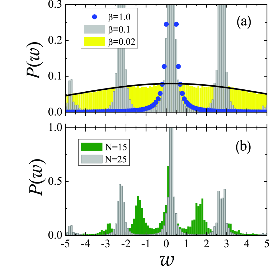
Figure 2: (Color online)  The probability distribution ${\cal P}(w)$ of the collective work performed on $N$ spinless fermions by a sudden switch of the magnetic flux from $f=0$ to $f=0.1$. In panel (a) results are displayed for the average number of particles $N=25$ at three different temperatures. The solid line represents the high temperature Gaussian approximation Eq. (8) for $\beta=0.02$. Panel (b) displays the distributions for two different average particle numbers at inverse temperature $\beta=0.1$. Note that for the larger $N$ value the side peaks have a larger distance from the central peak.

The chemical potential $\mu$ should be determined to satisfy

$$\langle{\cal N}\rangle=\sum_{k}\frac{1}{1+e^{\beta(E_{k}-\mu)}},$$ (15)

where $\langle{\cal N}\rangle$ is the average number of particles, which will be denoted as $N$ hereafter.

Figure 2 shows the work distributions for the flux $f=0.1$, at different temperatures and particle-numbers. As shown in Fig. 2(a) at low temperatures (large $\beta$), the distribution is narrow and centered at the difference between the ground-state energies in presence and absence of the magnetic flux which is given by $w_{c}=\sum_{k\in k_{gs}}(f^{2}-2kf)$. Here the summation runs over the $k$-values given by $k_{gs}=0,\pm 1,\cdots,\pm(N-1)/2$ for odd $N$. Due to the pairwise cancelation of positive and negative $k$-values in $w_{c}$, the term linear in $f$ vanishes, and hence $w_{c}=Nf^{2}$. For the used parameters $N=25$ and $f=0.1$, $w_{c}=0.25$ which indeed coincides with the central peak positions in Fig. 2(a). At higher temperatures (see $\beta=0.1$ in Fig. 2a), excited states of $k=\pm(N+1)/2$ come into play, which lead to side peaks located at $w_{s}=w_{c}\pm(N+1)f$. The number dependence of the side peak positions can be seen in Fig. 2(b): With decreasing particle numbers the distances between the central peak and the side peaks shrink. At high-temperatures, many excited levels contribute to the work fluctuation with almost equal weights. This leads to the seemingly continuous and flat distribution as displayed for $\beta=0.02$ in Fig. 2(a). In this case, in fact, particles follow the Maxwell-Boltzmann statistics, and the energy spectrum can be conceived as a continuum. Then, the characteristic function is approximately given by the products of $N$ single particle contributions, i.e., by ${\cal G}_{c}(u)\approx G_{c}^{N}(u)$. This gives ${\cal P}_{c}(w)\approx\sqrt{\beta/(4\pi Nf^{2})}e^{-\beta(w-Nf^{2})^{2}/(4Nf^{2})}$ which is plotted as solid line for $\beta=0.02$ in Fig. 2(a).

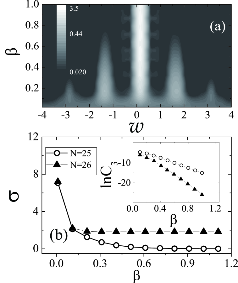
Figure 3: (Color online)  (a) The probability distribution of work $w$ for $N=15$ under a sudden magnetization flux switch from $f=0$ to $f=0.1$ is displayed as a function of $w$ and the inverse temperature $\beta$ by means of different gray-values as specified in the left upper part of the panel. At low temperatures the distribution is unimodal and develops side peaks with increasing temperature. (b) The temperature dependence of the standard deviation of work $\sigma$ is compared for $N=25$ and $N=26$. In the case of the even average particle number the standard deviation saturates at a finite value with decreasing temperature while it vanishes for the odd average particle number. The inset shows the natural logarithm of the third cummulant ($C_{3}$) versus $\beta$.

We present the temperature dependence of the probability distribution in Fig. 3(a). It displays the change from a narrow unimodal distribution at low temperatures through a multiply peaked distribution at intermediate temperatures to a broad Gaussian distribution at high temperatures. From the characteristic function of work one obtains the variance and all $n$th-order cummulants, $C_{n}$ via the formula, $C_{n}=(-i)^{n}\partial_{u}^{n}\ln{\cal G}(u)|_{u=0}$, where $\partial_{u}^{n}$ denotes the $n$th derivative with respect to $u$. As shown in Fig. 3(b) the variance and the third order cummulant for $N=25$ rapidly decrease to zero with decreasing temperature. The inset shows the exponential temperature dependence of $C_{3}$. We note that also the variance $\sigma^{2}=C_{2}$ decays exponentially with temperature, although we do not shown it here. On the other hand, for $N=26$ the variance saturates to a finite value, while the third moment exhibits an exponential decay, similarly to, but far faster than for the case when $N=25$.

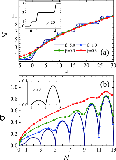
Figure 4: (Color online)  (a) The average number of particles as a function of the chemical potential for various temperatures. The stepwise increase of $N$ can be seen at low temperatures (see the curve for $\beta=5.0$ and the inset for $\beta=20$). (b) The number dependence of the standard deviation of the work at $f=0.1$. At the low temperatures $\sigma$are displays narrow dips at odd $N$ and broad peaks at even $N$. At the lowest temperature $\beta=20$ shown in the inset the standard deviation is vanishingly small up to $N=1$ and then displays a maximum at $N=2$, see the inset. At high temperatures ($\beta=0.3$), those structures are washed out at small and intermediate $N$ and become visible only for sufficiently large $N$.

The explicit form of the variance for the system is given by

$$\sigma^{2}=\sum_{k}[(1-\langle{\cal N}_{k}\rangle)\langle{\cal N}_{k}\rangle\Delta^{2}_{k}(f)]$$ (16)

which indicates that the number fluctuations $(1-\langle{\cal N}_{k}\rangle)\langle{\cal N}_{k}\rangle$ determine the variance of the work. The total average number $N$ of particles in the initial equilibrium state in absence of a magnetic flux is given by Eq. (15). At low temperatures it increases in a stepwise fashion with varying $\mu$ and forms plateaux of height $N=2n+1$ with steps close to $\mu=n^{2}$ (see Fig. 4(a)). This behavior is a direct consequence of the degeneracy of states with angular momentum $\pm k$. Due to the jumps, a system with an even average number of particles has pronounced work fluctuations that persist with decreasing temperature whereas for an odd number the variance of work vanishes with decreasing temperature. We present the number dependence of the standard deviation in panel (b) of Fig.4. At the low temperature ($\beta=5.0$), $\sigma$ vanishes at odd $N$ (except $N=1$), whereas it has peaks at even $N$’s. As the temperature increases, the dips and peaks at small and intermediate average numbers $N$ merge into a smooth and increasing curve but remain visible at sufficiently large values of $N$.

VI Summary and concluding remarks

In summary, we investigated the work distribution of many non-interacting fermionic particles driven by an AB flux in a non-simply connected geometry. In the single-particle case the work distribution at high-temperatures, namely, in the classical regime, is given by a Gaussian distribution, yielding $\langle e^{-\beta w}\rangle$=1, indeed confirming that the quantum flux leaves the free energy unchanged. By contrast, the distribution in the quantum regime is found to be multimodal caused by particle excitations. In particular, in order to deal with a many-particle system, we have generalized the expression for the characteristic function of work to quantum systems that initially are in a grand canonical state. We proved that the difference of the grand potentials of a hypothetical grand canonical equilibrium system with the initial temperature and chemical potential at the at the final parameter values and of the actual initial system enters a generalized Jarzynski equality. Although an energy measurement is an experimentally challenging task, theoretical examination of work in quantum many-particle systems per se is worthwhile for the fundamental understanding of nonequilibrium characteristics.

Acknowledgments. This work was supported by the National Research Grant funded by the Korean Government (NRF-2010-013-C00015), and the Volkswagen Foundation (project I/80424).

References

- (1) Y. Aharonov and D. Bohm, Phys. Rev. 115, 485 (1959).
- (2) Y. Aharonov and A. Casher, Phys. Rev. Lett. 53, 319 (1984).
- (3) C. R. Hagen, Phys. Rev. Lett. 64, 2347 (1990).
- (4) A. V. Balatsky and B. L. Altshuler, Phys. Rev. Lett. 70, 1678 (1993).
- (5) M. Wilkens, Phys. Rev. Lett. 72, 5 (1994).
- (6) C. Jarzynski, Phys. Rev. Lett. 78, 2690 (1997).
- (7) C. Jarzynski, C. R. Phys. 8, 495 (2007).
- (8) F. Douarche, S. Ciliberto, A. Petrosyan, and I. Rabbiosi, Europhys. Lett. 70, 593 (2005).
- (9) C. Bustamante, J. Liphardt and F. Ritort, Phys. Today 58 (7) 43 (2005).
- (10) V.Blickle, T. Speck, L. Helden, U. Seifert, and C. Bechinger, Phys. Rev. Lett. 96, 070603 (2006).
- (11) P. Pradhan, Phys. Rev. E 81, 021122 (2010).
- (12) H. Tasaki, arXiv:cond-mat/0009244.
- (13) S. Mukamel, Phys. Rev. Lett. 90, 170604 (2003).
- (14) M. Esposito and S. Mukamel, Phys. Rev. E 73, 046129 (2006).
- (15) W. De Roeck and C. Maes, Phys. Rev. E 69, 026115 (2004).
- (16) P. Talkner, E. Lutz, and P. Hänggi, Phys. Rev. E 75, 050102(R) (2007).
- (17) P. Talkner and P. Hänggi, J. Phys. A 40, F569 (2007).
- (18) P. Talkner, P. Hänggi, and M. Morillo, Phys. Rev. E 77, 051131 (2008).
- (19) P. Talkner, P. S. Burada, and P. Hänggi, Phys. Rev. E 78, 011115 (2008).
- (20) P. Talkner, P. S. Burada, and P. Hänggi, Phys. Rev. E. 79, 039902 (2009).
- (21) S. Deffner and E. Lutz, Phys. Rev. E 77, 021128 (2008).
- (22) M. Campisi, P. Talkner, and P. Hänggi, Phys. Rev. Lett. 102, 210401 (2009).
- (23) M. Esposito, U. Harbola, S. Mukamel, Rev. Mod. Phys. 81, 1665 (2009).
- (24) M. Campisi, P. Hänggi, P. Talkner, arXiv:1012.2268.
- (25) R. Landauer and M. Büttiker, Phys. Rev. Lett. 54, 2049 (1985).
- (26) V. Chandrasekhar, R. A. Webb, M. J. Brady, M.B. Ketchen, W. J. Gallagher, and A. Kleinsasser, Phys. Rev. Lett. 67, 3578 (1991).
- (27) M. Y. Choi, Phys. Rev. Lett. 71, 2987 (1993).
- (28) D. Loss and P. Goldbart, Phys. Rev. B 43, 13762 (1991).
- (29) A. C. Bleszynski-Jayich, W. E. Shanks, B. Peaudecerf, E. Ginossar, F. von Oppen, L. Glazman, and J. G. E Harris, Science 326, 272 (2009).
- (30) In order to make the -peaks visible we introduce a small positive number and plotted with if , and , otherwise.
- (31) P. Talkner, M. Campisi, P. Hänggi, J. Stat. Mech.: Theory Exp. P02025 (2009).
- (32) T. Schmiedle and U. Seifert, J. Chem. Phys. 126, 044101 (2007).
- (33) K. Saito, Y. Utsumi, Phys. Rev B 78, 115429 (2008).
- (34) D. Andrieux, P. Gaspard, T. Monnai, and S. Tasaki, New J. Phys. 11, 043014 (2009).
- (35) M. Campisi, P. Talkner, P. Hänggi, Phys. Rev. Lett. 105, 140601 (2010).