A needlet ILC analysis of WMAP 7-year data: estimation of CMB temperature map and power spectrum

Abstract

The WMAP satellite has provided high resolution, high signal to noise ratio maps of the sky in five main frequency bands ranging from $23$ to $94$ GHz. These maps consist in noisy observations a mixture of Cosmic Microwave Background (CMB) anisotropies and of other astrophysical foreground emissions. We present a new foreground-cleaned CMB map, as well as a new estimation of the angular power spectrum of CMB temperature anisotropies, based on $7$ years of observations of the sky by WMAP. The method used to extract the CMB signal is based on an implementation of minimum variance linear combination of WMAP channels and of external full-sky foreground maps, on a frame of spherical wavelets called needlets. The use of spherical needlets makes possible localised filtering both in pixel space and harmonic space, so that the ILC weights are adjusted as a function of location on the sky and of angular scale. Our CMB power spectrum estimate is computed using cross power spectra between CMB maps obtained from different individual years of observation. The CMB power spectrum is corrected for low-level biases originating from the ILC method and from foreground residual emissions, by making use of realistic simulations of the whole analysis pipeline. Our error bars, compatible with those obtained by the WMAP collaboration, are obtained from the combination of two terms: the internal scatter of individual $C_{\ell}$ in each $\ell$ bin, and a term originating from uncertainties in our correction for biases due to empirical correlations between CMB and foregrounds, as well as to residual foregrounds in the CMB maps. Our power spectrum is essentially compatible, within error bars, with the result obtained by the WMAP collaboration, although it is systematically lower at the lowest multipoles, more than expected considering that the two estimates are based on the same original data. Exhaustive investigations of the presence of a possible bias in our estimate fail to explain the difference. Comparison with several other analyses confirm the existence of differences in the large scale CMB power, which are significant enough that until the origin of this discrepancy is understood, some caution is recommended in scientific work relying much on the exact value of the CMB power spectrum in the Sachs-Wolfe plateau.

1 Introduction

Cosmic Microwave Background (CMB) anisotropies provide a snapshot of what the universe looked like at the moment of recombination. The statistical properties of CMB fluctuations depend on the original primordial perturbations from which they arose, as well as on the subsequent evolution of the universe as a whole. This makes the precise measurement of CMB power spectra, both in temperature and polarisation, a gold mine for understanding and describing the universe from early times to now.

For cosmological models in which initial perturbations are Gaussian, the information carried by CMB anisotropies is completely characterised by the multivariate angular power spectrum of the observations (i.e. the auto and cross power spectra of temperature and polarisation maps). The angular power spectrum of the CMB is sensitive to the values of the different cosmological parameters which primarily describe the fundamental properties of the universe, such as its matter content, age, expansion history, global geometry and the properties of the initial fluctuations that seeded the large scale structure observable today. The possibility to use this for constraining the cosmological parameters hinges upon the existence of acoustic oscillations in the primordial plasma before last scattering of CMB photons, and on the ability of CMB experiments to disentangle such primordial fluctuations from those induced by cosmic structures at lower redshift. This is why a key goal of the CMB community is to measure the true CMB temperature anisotropies and polarisation in the sky.

Since the discovery of the CMB by Penzias & Wilson (1965), tremendous efforts on the instrumental side have been made to improve sensitivity and angular resolution of CMB experiments. Recently, multi-frequency data for the complete sky have become available from 7 years of observation with the WMAP space mission (Jarosik et al., 2010). WMAP confirmed the leading theory in cosmology, the $\Lambda$CDM (cold dark matter) model of a universe governed by Einstein’s theory of general relativity, and the evolution of which is dominated by the impact of a cosmological constant $\Lambda$, equivalent to a contribution, in the total energy density, of vacuum energy, or more generally ‘dark energy’ (Larson et al., 2011; Komatsu et al., 2010).

The WMAP data has already allowed a determination of several central cosmological parameters with good accuracy. These determinations are based on a number of simplicity assumptions, which need to be tested by more accurate and extensive measurements. The Planck satellite of the European Space Agency, next generation CMB space mission after WMAP, surpasses its predecessor in resolution, sensitivity and frequency coverage (Tauber et al., 2010; Planck Collaboration et al., 2011), and will provide an update of the present picture and of cosmological parameter estimates in early 2013.

Determining the cosmological parameters with CMB experiments, however, requires careful cleaning of the CMB maps from contamination by galactic and extra-galactic foregrounds. In the low frequency microwave regime (below about 100 GHz) the strongest contamination comes from galactic synchrotron and free-free emission. At higher frequencies, where synchrotron and free-free emissions are low, dust emission dominates. In addition, extragalactic point-like sources are a significant contaminant at high galactic latitude and on small scale. Even when the brightest sources are identified and subtracted-out or masked, their residual contribution may dominate over the cosmic variance uncertainty on small angular scales, and bias the measurement of the CMB power spectrum (see Delabrouille & Cardoso (2009) for a review on component separation in CMB observations).

Most of the foreground emissions are strongly correlated between frequency channels. Except for the very faint kinetic SZ signal, the underlying frequency dependences of the emissions differ from that of the CMB anisotropies. Exploiting this facts, a model-independent method to remove foregrounds from the multi-frequency observations of CMB, the so-called ‘Internal Linear Combination’ (ILC), has been proposed to extract the CMB signal from the multi-frequency data such as that of WMAP or Planck (see, e.g., Tegmark & Efstathiou (1996)). The idea behind the ILC method is to find the linear combination of the available maps which has minimal variance while retaining unit response to the CMB. The main advantage of this foreground cleaning method is that it does not require any assumption about the foregrounds. Another advantage is that it is easy to implement, and computationally fast. Finally, it can be extended to impose the rejection of a particular foreground if needed (Remazeilles et al., 2011a), or to extract the total combined emission of several correlated foregrounds (Remazeilles et al., 2011b).

There are, however, also drawbacks to the method. As discussed by a number of authors (Hinshaw et al., 2007; Saha et al., 2008; Delabrouille & Cardoso, 2009; Delabrouille et al., 2009), the component of interest (the CMB in our case) and foreground signals must be uncorrelated for proper ILC performance. This can be, on finite data sets, only approximately true, and empirical correlations between the CMB and foregrounds generate a bias in the reconstructed CMB. In addition, as shown by Dick et al. (2010), the ILC method tends to amplify calibration errors, and reconstruct a CMB map which can be largely under-calibrated, in particular for high signal-to-noise ratio observations. These sources of error must be monitored carefully in the analysis of CMB maps obtained in this way.

In this paper, we address the problem of measuring as precisely as possible the CMB temperature power spectrum from WMAP 7-year observations, with close to minimal noise and contamination by foreground emission. The paper is organised as follows: In section 2 we describe the methodology to estimate the CMB and its power spectrum using an ILC on wavelet decompositions of sky maps observed at different frequencies. The implementation of this on WMAP 7-year data is described in section 3 and section 4. The results are discussed in section 5. We conclude in section 6.

2 The Needlet ILC

Component separation with an ILC method can straightforwardly be performed in real space or in harmonic space. By this we mean that different ILC weights can be computed in different regions of the sky, or in different regions of harmonic space. This allows for variations of the data covariance matrix in either space.

The ILC in harmonic space however does not take into account the fact that noise is the dominant source of CMB measurement error at high galactic latitude while foreground signals dominate at low galactic latitude. On the other hand, the ILC in pixel space does not take into account the fact that noise dominates at high angular frequency (small scales) while foreground emission dominates on large scales. In order to overcome this problem, we follow the approach of Delabrouille et al. (2009) and implement the ILC on a frame of spherical wavelets, called needlets. This special type of spherical wavelets allows localised filtering in both pixel space and harmonic space because they have compact support in the harmonic domain, while still being very well localised in pixel domain (Narcowich et al., 2006; Marinucci et al., 2008; Guilloux et al., 2009). Needlets have already been used in various analyses of WMAP data besides component separation and power spectrum estimation, for instance by Pietrobon et al. (2008) to detect features in the CMB, and by Rudjord et al. (2009) to put limits on the non-gaussianity parameter $f_{\rm NL}$.

Various versions of the ILC on WMAP data have been implemented by a number of authors so far (Tegmark et al., 2003; Eriksen et al., 2004; Hinshaw et al., 2007; Park et al., 2007; Saha et al., 2008; Delabrouille et al., 2009; Kim et al., 2009; Souradeep, 2011). Alternate component separation on WMAP data has been performed using independent component analysis methods such as SMICA (Patanchon et al., 2005), CCA (Bonaldi et al., 2007), and FASTICA (Maino et al., 2007; Bottino et al., 2008, 2010). Specific analyses to extract foreground component emissions have permitted to isolate the total foreground contamination (Ghosh et al., 2011) or detect the thermal SZ emission of galaxy clusters (Atrio-Barandela et al., 2008; Melin et al., 2011).

2.1 The data model

A CMB space mission such as WMAP provides full-coverage, multi-frequency anisotropy maps of the sky $T^{\text{OBS},c}(\hat{n})$ in $n_{c}$ different frequency bands (channels). The observed signal $T^{\text{OBS},c}(\hat{n})$ in channel $c$ can be modelled as,

$$T^{\text{OBS},c}(\hat{n})=\int_{\hat{n}^{\prime}}d\Omega_{\hat{n}^{\prime}}\,\,B^{c}(\hat{n},\hat{n}^{\prime})\,\,T^{\text{SIG},c}(\hat{n}^{\prime})+T^{\text{N},c}(\hat{n}),$$ (1)

where $T^{\text{SIG},c}(\hat{n})$ is the signal (sky) component, itself decomposed in the sum of CMB and foreground components,

$$T^{\text{SIG},c}(\hat{n})=a^{c}\,T^{\text{CMB}}(\hat{n})+T^{\text{FG},c}(\hat{n}),$$ (2)

$a^{c}$ being the CMB calibration coefficient for the channel $c$. Up to calibration uncertainties, $a^{c}=1$ for all WMAP channels. If, in addition to WMAP data, we use extra ancillary data which serve as foreground templates to help foreground subtraction, as done in the present work, the coefficients $a^{c}$ vanish for such data sets.

The beam function $B^{c}(\hat{n},\hat{n}^{\prime})$ represents the smoothing of the signal due to the finite resolution of the observations. The beam is assumed here to be circularly symmetric, i.e., $B^{c}(\hat{n},\hat{n}^{\prime})$ depends only on the angle $\theta=\cos^{-1}(\hat{n}.\hat{n}^{\prime})$ between the directions $\hat{n}$ and $\hat{n}^{\prime}$. We may then expand this function in terms of Legendre polynomials,

$$B^{c}(\hat{n},\hat{n}^{\prime})=\sum_{l=0}^{\infty}\frac{2l+1}{4\pi}B_{l}^{c}P_{l}(\hat{n}.\hat{n}^{\prime}).$$ (3)

The term $T^{\text{N},c}(\hat{n})$ in equation 1 represents the detector noise in channel $c$. Unlike the CMB and foreground components, instrumental noise is not affected by the beam function.

Equation 1 can be recast, in the spherical harmonic representation, as:

$$a_{lm}^{\text{OBS},c}=a^{c}\,B_{l}^{c}\,a_{lm}^{\text{CMB}}+B_{l}^{c}\,a_{lm}^{\text{FG},c}+a_{lm}^{\text{N},c}.$$ (4)

2.2 Implementation of the needlet transform

Considering that each channel observes the sky at a different resolution, the maps are first convolved/deconvolved, in harmonic space, to the same resolution:

$$a_{lm}^{c}=\frac{B_{l}}{B_{l}^{c}}\,\,a_{lm}^{\text{OBS},c}.$$ (5)

Each of these maps $a_{lm}^{c}$ is then decomposed into a set of filtered maps $a_{lm}^{c,j}$ represented by the spherical harmonic coefficients,

$$a_{lm}^{c,j}=h_{l}^{j}a_{lm}^{c}.$$ (6)

The filters $h_{l}^{j}$ is chosen in such a way that

$$\sum_{j}\left(h_{l}^{j}\right)^{2}=1,$$ (7)

which permits us to directly reconstruct the original maps $a_{lm}^{c}$ from their filtered maps $a_{lm}^{c,j}$ using the same set of filters. In terms of $h_{l}^{j}$, the spherical needlets are defined as,

$$\Psi_{jk}(\hat{n})=\sqrt{\lambda_{jk}}\sum_{l=0}^{l_{\max}}\sum_{m=-l}^{l}h_{l}^{j}\,Y_{lm}^{*}(\hat{n})\,Y_{lm}(\hat{\xi}_{jk}),$$ (8)

where $\{\xi_{jk}\}$ denote a set of cubature points on the sphere, corresponding to a given scale $j$. In practice, we identify these points with the pixel centres in the HEALPix pixelisation scheme (Górski et al., 2005). The cubature weights $\lambda_{jk}$ are inversely proportional to the number $N_{j}$ of pixels used for the needlet decomposition at scale $j$, i.e. $\lambda_{jk}=\frac{4\pi}{N_{j}}$. The needlet coefficients for CMB temperature anisotropies $T(\hat{n})=\sum_{l=0}^{l_{\max}}\sum_{m=-l}^{l}a_{lm}Y_{lm}(\hat{n})$ are denoted as,

$$\beta_{jk} = \int_{S^{2}}T(\hat{n})\,\Psi_{jk}(\hat{n})\,d\Omega_{\hat{n}}$$ (9)

$$= \sqrt{\lambda_{jk}}\sum_{l=0}^{l_{\max}}\sum_{m=-l}^{l}h_{l}^{j}\,B_{l}\,a_{lm}\,\,Y_{lm}(\xi_{jk}).$$

The linearity of the needlet decomposition implies that the needlet coefficients $\beta_{jk}^{c}$ corresponding to the filtered map obtained from the harmonic coefficients $a_{lm}^{c,j}$ are a linear combination of the needlet coefficients of individual components and noise at HEALPix grid points $\xi_{jk}$:

$$\beta_{jk}^{c}=a^{c}\,\beta_{jk}^{\text{CMB}}+\beta_{jk}^{\text{FG},c}+\beta_{jk}^{\text{N},c}$$ (10)

where,

$$\beta_{jk}^{\text{CMB}} = \sqrt{\lambda_{jk}}\sum_{l=0}^{l_{\max}}\sum_{m=-l}^{l}h_{l}^{j}\,B_{l}\,a_{lm}^{\text{CMB}}\,\,Y_{lm}(\xi_{jk})$$

$$\beta_{jk}^{\text{FG},c} = \sqrt{\lambda_{jk}}\sum_{l=0}^{l_{\max}}\sum_{m=-l}^{l}h_{l}^{j}\,B_{l}\,a_{lm}^{\text{FG},c}\,\,Y_{lm}(\xi_{jk})$$

$$\beta_{jk}^{\text{N},c} = \sqrt{\lambda_{jk}}\sum_{l=0}^{l_{\max}}\sum_{m=-l}^{l}h_{l}^{j}\,\frac{B_{l}}{B_{l}^{c}}\,a_{lm}^{\text{N},c}\,\,Y_{lm}(\xi_{jk})$$ (11)

2.3 Implementation of the needlet ILC

The ILC estimate of needlet coefficients of the cleaned map is obtained as a linearly weighted sum of the needlet coefficients $\beta_{jk}^{c}$,

$$\beta_{jk}^{\text{NILC}}=\sum_{c=1}^{n_{c}}\omega_{jk}^{c}\,\beta_{jk}^{c}$$ (12)

where $\omega_{jk}^{c}$ is the needlet weight for the scale $j$ and the frequency channel $c$ at the pixel $k$. Under the assumption of de-correlation between CMB and foregrounds, and between CMB and noise, the empirical variance of the error is minimum when the empirical variance of the ILC map itself is minimum. The condition for preserving the CMB signal during the cleaning is encoded as the constraint:

$$\sum_{c=1}^{n_{c}}a^{c}\omega_{jk}^{c}=1.$$ (13)

The resulting needlet ILC weights $\widehat{\omega}_{jk}^{c}$ that minimise the variance of the reconstructed CMB, subject to the constraint that the CMB is preserved, are expressed as:

$$\widehat{\omega}_{jk}^{c}=\frac{\sum_{c^{\prime}=1}^{n_{c}}\left(\widehat{R}_{jk}^{-1}\right)^{cc^{\prime}}a^{c^{\prime}}}{\sum_{c=1}^{n_{c}}\sum_{c^{\prime}=1}^{n_{c}}a^{c}.\left(\widehat{R}_{jk}^{-1}\right)^{cc^{\prime}}a^{c^{\prime}}}$$ (14)

The NILC estimate of the cleaned CMB needlet coefficients is:

$$\beta_{jk}^{\text{NILC}}=\beta_{jk}^{\text{CMB}}+\frac{\sum_{c=1}^{n_{c}}\sum_{c^{\prime}=1}^{n_{c}}\left(\beta_{jk}^{\text{FG},c}+\beta_{jk}^{\text{N},c}\right)\left(\widehat{R}_{jk}^{-1}\right)^{cc^{\prime}}\,a^{c^{\prime}}}{\sum_{c=1}^{n_{c}}\sum_{c^{\prime}=1}^{n_{c}}a^{c}\left(\widehat{R}_{jk}^{-1}\right)^{cc^{\prime}}a^{c^{\prime}}}$$

where $\widehat{R}_{jk}^{cc^{\prime}}$ are empirical estimates of the elements of covariance matrix $R_{jk}^{cc^{\prime}}=\left<\beta_{jk}^{c}\beta_{jk}^{c^{\prime}}\right>$ for scale $j$ at pixel $k$. Those estimates are obtained each as an average of the product of the relevant computed needlet coefficients over some space domain ${\cal D}_{k}$ centred at $k$. In practice, they are computed as

$$\widehat{R}_{jk}^{cc^{\prime}}=\frac{1}{n_{k}}\sum_{k^{\prime}}w_{j}(k,k^{\prime})\beta_{jk}^{c}\beta_{jk}^{c^{\prime}},$$ (15)

where the weights $w_{j}(k,k^{\prime})$ define the domain ${\cal D}_{k}$. A sensible choice is for instance $w_{j}(k,k^{\prime})=1$ for $k^{\prime}$ closer to $k$ than some limit angle, and $w_{j}(k,k^{\prime})=0$ elsewhere, or alternatively, $w_{j}(k,k^{\prime})$ shaped as a Gaussian beam of some given size that depends on the scale $j$ (which is what we do here).

Finally, the NILC estimate of the cleaned CMB map can be reconstructed from cleaned CMB needlet coefficients using the same set of filters that was used to decompose the original maps into their needlet coefficients. The NILC CMB temperature map is then

$$T^{\text{NILC}}(\hat{n}) = \sum_{lm}a_{lm}^{\text{NILC}}\,Y_{lm}(\hat{n})$$ (16)

$$= \sum_{lm}\,\left(B_{l}\,a_{lm}^{\text{CMB}}+a_{lm}^{\text{RFG}}+a_{lm}^{\text{RN}}\right)\,Y_{lm}(\hat{n}),$$

where the harmonic coefficients residual foreground ($a_{lm}^{\text{RFG}}$) and residual noise($a_{lm}^{\text{RN}}$) are given by:

$$a_{lm}^{\text{RFG}}=\sum_{j}\sum_{k}\sqrt{\lambda_{jk}}\,\beta_{jk}^{\text{RFG}}\,h_{l}^{j}\,Y_{lm}(\xi_{jk})$$ (17)

and

$$a_{lm}^{\text{RN}}=\sum_{j}\sum_{k}\sqrt{\lambda_{jk}}\,\beta_{jk}^{\text{RN}}\,h_{l}^{j}\,Y_{lm}(\xi_{jk}).$$ (18)

Equation 16 implies that the NILC estimate of CMB contains some residual foreground and noise contamination.

3 WMAP 7 year needlet ILC map

The WMAP satellite has observed the sky in five frequency bands denoted K, Ka, Q, V and W, centred on the frequencies of 23, 33, 41, 61 and 94 GHz respectively. After $7$ years of observation, the released data includes maps obtained with ten difference assemblies, for $7$ individual years. One map is available, per year, for each of the K and Ka bands, two for the Q band, two for the V band and four for the W band. These sky maps are sampled using the HEALPix pixelisation scheme at a resolution level (nside  1024), corresponding to approximately $12$ million sky pixels.

In a first step, for each frequency band, we average all the difference-assembly maps obtained at the same frequency. This yields $5$ band-averaged maps. However, contrarily to the 7-year average maps at nside = 512 also provided by WMAP, these maps at nside = 1024 are not offset corrected. In order to determine the values of the offset for a particular frequency band, we have used standard resolution 7-year band-average maps of WMAP as references. Offset values, for all frequency bands, are obtained by determining the mean of the difference between the band-averaged map being considered (degraded to nside = 512), and the released ‘reference’ map. We implement the needlet ILC on these offset-corrected maps.

In addition to these maps, we use three foreground templates in our analysis: dust at 100 microns, as obtained by Schlegel et al. (1998), the 408 MHz synchrotron map of Haslam et al. (1981), and the composite all-sky H-alpha map of Finkbeiner (2003). The offset-corrected WMAP maps and fore-mentioned foreground templates are convolved/deconvolved, in harmonic space, to a common beam resolution (corresponding to that of the W frequency channel of WMAP 7-year release) before the implementation of the needlet ILC on the map set.

Each of these maps is decomposed into a set of needlet coefficients. For each scale $j$, needlet coefficients of a given map are stored in the format of a single HEALPix map at degraded resolution. The filters $h^{j}_{l}$ used to compute filtered maps are shaped as follows:

$$h^{j}_{l}=\left\{\begin{array}[]{rl}\cos\left[\left(\frac{l^{j}_{peak}-l}{l^{j}_{peak}-l^{j}_{min}}\right)\frac{\pi}{2}\right]&\text{for }l^{j}_{min}\leq l<l^{j}_{peak},\\ \\ 1&\text{for }l=l_{peak},\\ \\ \cos\left[\left(\frac{l-l^{j}_{peak}}{l^{j}_{max}-l^{j}_{peak}}\right)\frac{\pi}{2}\right]&\text{for }l^{j}_{peak}<l\leq l^{j}_{max}\end{array}\right.$$

For each scale $j$, the filter has compact support between the multipoles $l^{j}_{min}$ and $l^{j}_{max}$ with a peak at $l^{j}_{peak}$ (see figure 1 and table 1). The needlet coefficients $\beta_{jk}$ are computed from these filtered maps on HEALPix grid points $\xi_{jk}$ with resolution parameter nside equal to the smallest power of $2$ larger than $l^{j}_{max}/2$.

Table 1: List of needlet bands used in the present analysis.

Band index	$l_{min}$	$l_{peak}$	$l_{max}$	nside
1	0	0	50	32
2	0	50	100	64
3	50	100	150	128
4	100	150	250	128
5	150	250	350	256
6	250	350	550	512
7	350	550	650	512
8	550	650	800	512
9	650	800	1100	1024
10	800	1100	1500	1024

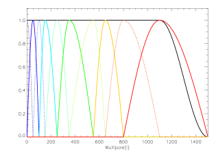
Figure 1: Needlet bands used in the present analysis. The black line shows the normalisation of the needlet bands, i.e. the total filter applied to the original map after needlet decomposition and synthesis of the output map from needlet coefficients.

The estimates of needlet coefficients covariance matrices, for each scale $j$, are computed by smoothing all possible products of needlet coefficient maps $\beta^{c}_{jk}\beta^{c^{\prime}}_{jk}$ with Gaussian beams. In this way, an estimate of needlet covariances at each point $k$ is obtained as a local, weighted average of needlet coefficient products. The process is summarised by the diagram:

$$\{\beta^{c}_{jk}\beta^{c^{\prime}}_{jk}\}_{k=1,..,N_{pix}}\,\xrightarrow{\text{SHT}}\,\{a^{c\,c^{\prime}}_{lm}\}_{l=0,l^{j}_{max},m=-l,..,0,..,l}$$

$$\Big{\downarrow}{\times}\hskip 72.26999pt$$

$$\{\hat{R}^{c\,c^{\prime}}_{jk}\}_{k=1,..,N_{pix}}\xleftarrow{\text{SHT}^{-1}}\,\{B^{j}_{l}a^{c\,c^{\prime}}_{lm}\}_{l=0,l^{j}_{max},m=-l,..,0,..,l}$$

The full width at half maximum (FWHM) of each of the Gaussian windows used for this purpose is chosen to ensure the computation of the statistics by averaging about 1200 samples or more. Choosing a smaller FWHM results in excessive error in the covariance estimates, and hence excessive bias. Choosing a larger FWHM results in less localisation, and hence some loss of effectiveness of the needlet approach.

Using these covariance matrices, the ILC solution for each scale is implemented locally to get the needlet weights and hence the estimated CMB needlet coefficients. Finally, a full sky CMB map, displayed in figure 2, is synthesised from these estimated needlet coefficients.

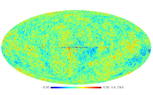
Figure 2: The NILC estimate of CMB temperature anisotropies obtained by implementing the NILC on the 7-year band average maps (at nside = 1024) provided by the WMAP collaboration.

4 CMB angular power spectrum

Component separation with a needlet ILC is the first step in our analysis. The cleaned CMB map, however, still contains residuals of noise and foreground emission, and is impacted by the ILC bias due to empirical correlations of CMB and foregrounds as well as by the effect of calibration uncertainties and beam uncertainties. Residual contamination is clearly visible, for instance, along a narrow strip on the Galactic plane of the map displayed in figure 2.

In the following, we discuss these various types of errors, and our strategy to minimise or evaluate their impact on the estimation of the CMB power spectrum.

4.1 Impact of instrumental noise

It would be possible to use the estimated noise level in the WMAP maps to de-bias the power spectrum of the map obtained in section 3 from instrumental noise contribution. This, however, requires, in particular at high multipoles, a very accurate estimate of the noise level.

Thus, instead of trying to de-bias from instrumental noise a single power spectrum (computed on a single NILC map averaging all seven years of data), we produce independent CMB maps for each of the individual $7$ years of observations, and compute the CMB power spectrum as an average of the $21$ cross power spectra obtained from the $7$ clean CMB maps. In practice, all $7$ maps are obtained using the same set of needlet weights, determined using the co-added 7 year observations. Instrumental noise, being uncorrelated from year to year, does not bias the average power spectrum, and can be ignored in the estimate.

4.2 Impact of residual foregrounds

As the ILC weights used for all years are the same, residual foreground emission will be the same in all maps. These residuals, although small (as compared to original foreground contamination in the maps of the individual differencing assemblies), are thus 100% correlated between the different single year maps, and bias the CMB power spectrum. They are dealt with using a combination of masking and de-basing, as follows.

First of all, the impact of most of the contamination from residuals of bright point sources is removed from our estimate of power spectra by applying to our output CMB maps, for each individual year, the point source mask provided by the WMAP collaboration, and filling-in the holes by an interpolation procedure using the values of CMB anisotropies in the neighbouring unmasked pixels. We start with the masked border pixels, assign to each of them the average of all observed pixels which are within a distance of two pixel sizes. Then we iterate, increasing the distance for averaged pixels by two pixel sizes at each iteration. While not theoretically optimal, this procedure works very well in practice.

The impact of galactic contamination on our power spectrum estimate is limited by the use of a conservative galactic mask, $M_{\bar{\theta}_{r},\bar{\theta}_{w}}$(applied after the NILC, so that we still get full sky maps). Our mask simply excludes sky regions in which galactic residuals after component separation can be too strong for precise CMB power spectrum estimation. The apodised mask used in practice is:

$$M_{\bar{\theta}_{r},\bar{\theta}_{w}}(\theta,\phi)=\left\{\begin{array}[]{rl}0&\text{for }0^{\circ}\leq\left|\bar{\theta}\right|<\bar{\theta}_{r},\\ \\ \sin^{2}\left[\left(\frac{\bar{\theta}-\bar{\theta}_{r}}{\bar{\theta}_{w}}\right)\frac{\pi}{2}\right]&\text{for }\bar{\theta}_{r}\leq\left|\bar{\theta}\right|\leq\bar{\theta}_{r}+\bar{\theta}_{w},\\ \\ 1&\text{for }\left|\bar{\theta}\right|>\bar{\theta}_{r}+\bar{\theta}_{w}\\ \end{array}\right.$$

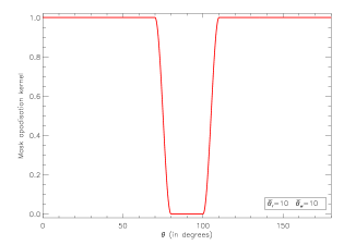
Figure 3: Apodisation kernel for Galactic mask used in our analysis

where $\bar{\theta}=\left(\frac{\pi}{2}-\theta\right)\frac{180^{\circ}}{\pi}$ is the latitude. The apodisation of the mask borders limits the aliasing of large scales into small scales.

4.3 Validation on simulations and de-biasing

The method is tested, tuned, and validated using numerical simulations based on the Planck Sky Model (PSM). A general description of the PSM can be found on the PSM web page, as well as in Leach et al. (2008) and/or in Betoule et al. (2009). The simulated sky emission comprises:

• a Gaussian CMB temperature map, with a power spectrum matching the WMAP best fit;

• galactic emission, consisting in the superposition of synchrotron, free-free, thermal dust, and spinning dust;

• SZ effects, both thermal and kinetic;

• a population of point sources.

Noise maps for the individual years are randomly generated with a Gaussian probability distribution that is uncorrelated from pixel to pixel and between different years. The noise variance per pixel is inversely proportional to the hit count for each individual year. This is expected to describe reasonably accurately the expected noise behaviour of the actual WMAP data. The noise level impacts the exact value of the NILC coefficients (in particular at high galactic latitude and on small scales), and the exact size of the error bars in the measured CMB power spectrum. Small uncertainties in the noise, however, do not bias the estimated $C_{\ell}$.

Biases are investigated in the following way. Fifty different realisations of the full simulations are generated, and processed in the exact same way as the actual WMAP data sets. The average systematic difference (i.e. bias) between the recovered power spectra and the input CMB power spectrum is computed. The bias estimated in this way (displayed with green right-facing triangles in figure 6) is typically less than $3-5$% of the estimated $C_{l}$, and also typically smaller than the total errors on individual $C_{l}$ bins (figure 6). This average bias is nonetheless corrected for in our estimate of the CMB power spectrum (see section 4.4 for details).

The observed bias is due to the combination of two effects: additive residual foreground emission, which generates a positive bias, and empirical correlations between contaminants (foregrounds and noise) and CMB maps which generate the negative ILC bias discussed at length in Delabrouille et al. (2009).

Our de-biasing procedure deserves a discussion, since using this average bias estimated on simulations to de-bias (by subtraction) the actual CMB power spectrum obtained on real WMAP data is valid only if the simulations are representative of the real sky, i.e.

• the CMB power spectrum assumed in the simulations must be close to the real one;

• the simulated foregrounds must be representative of the sky (similar levels and behaviour)

• the description of the instrument must be correct.

The real CMB power spectrum and the real foregrounds are not known to infinite accuracy (otherwise there would be no point in trying to measure them again). However, the following points give us confidence in the representativeness of our simulations:

• Concerning the CMB, a small error $\Delta C_{l}$ in the simulated CMB $C_{l}$ would generate a miscalculation of the multiplicative ILC bias. The error in this bias estimate, however, is of second order (of order 2% times $\Delta C_{l}$), with a minor impact on the $C_{l}$ estimate.

• The galactic foreground model in the PSM is built on the basis of the WMAP foreground analysis of Miville-Deschênes et al. (2008). Even if the model has known limitations and uncertainties, it yields sky emission in the WMAP channels that is in good agreement with the observations. For safety in our power spectrum estimation however, a conservative mask being applied to exclude the galactic plane region from the calculation of temperature $C_{l}$.

• PSM point sources are based on real observations of radio sources with GB6 (Gawiser et al., 1998), PMN (Griffith et al., 1994; Wright et al., 1994; Griffith et al., 1995; Wright et al., 1996), SUMSS (Mauch et al., 2003) and NVSS (Condon et al., 1998), and includes the full catalog of WMAP detected point sources. The PSM point source model is hence thought to be reasonably representative of the expected point source contamination in WMAP data sets.

• The thermal and kinetic SZ effects are very faint as compared to WMAP sensitivity, and do not play a significant role in this analysis.

• Uncertainties connected to the description of the instrument that are susceptible to impact our simulations are mostly calibration uncertainties and beam uncertainties. The impact of these, which turns out to be negligible as estimated on simulations, will be discussed later on.

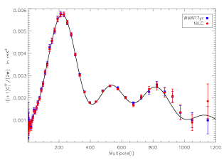
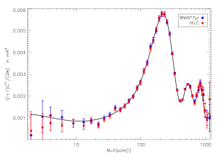
Figure 4: The red filled circles show the angular power spectrum estimated, after foreground subtraction with the NILC, using $7$ years of observations of WMAP. The blue filled squares show the 7-year angular power spectrum published by the WMAP collaboration. The black solid line shows the theoretical angular power spectrum for WMAP best-fit Lambda-CDM model. The top panel uses a linear scale in the horizontal axis, and the bottom panel a logarithmic scale. Our estimate is consistent with that of WMAP, although it has significantly less power at low multipoles ($l<15$).

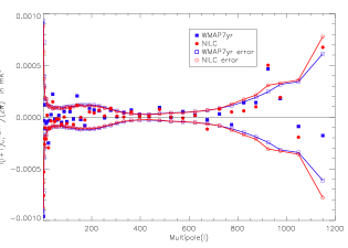
Figure 5: The red filled circles show the difference between the angular power spectrum estimated using NILC maps and the theoretical WMAP best fit angular power spectrum. The red open circles show the total error in the estimate of the angular power spectrum using our method. Similarly, the blue filled squares show the difference between the angular power spectrum published by the WMAP collaboration and theoretical best fit. The blue open squares show the error in the estimate of angular power spectrum provided by WMAP. The top panel uses a linear scale in the horizontal axis, and the bottom panel a logarithmic scale.

4.4 Power spectrum estimation

Residual noise in our CMB maps is inhomogeneous, primarily because of non-uniform sky coverage, with higher number of observations in the directions of ecliptic poles and rings around them of $45^{\circ}$ radius. Taking into account this inhomogeneity for computing the CMB power spectrum is expected to yield more precise estimates of the CMB $C_{l}$ in multipoles where the noise is the main source of error.

We follow the general idea of the noise-weighting using needlets described in Faÿ et al. (2008), with a number of changes to adapt the method to our present analysis. Consider a bin in $l$, defined by a window $H_{b}(l)=\left[h_{b}(l)\right]^{2}$ restricted to the range in $l$ limited by $l_{\rm min}^{b}$ and $l_{\rm max}^{b}$, such that

$$H_{b}(l)=\left\{\begin{array}[]{cl}\frac{l(l+1)}{2\pi}\frac{1}{(2l+1)}\frac{1}{(\Delta l)_{b}}&\;\;\;l_{min}^{b}\leq l\leq l_{max}^{b}\\ \\ 0&\;\;\;\text{otherwise}\\ \end{array}\right.$$

with $(\Delta l)_{b}=l_{\rm max}^{b}-l_{\rm min}^{b}+1$. The power $P_{b}$ of the CMB map filtered with $h_{b}(l)$ is an estimate of the CMB angular power spectrum $C_{\ell}$ in the window $H_{b}(l)$, with:

$$P_{b} = \sum_{l}H_{b}(l)(2l+1)C_{l}$$ (22)

$$= \frac{1}{(\Delta l)_{b}}\sum_{l}\frac{l(l+1)}{2\pi}C_{l}$$

Now starting from a pair of reconstructed CMB maps for two different years of observation $i$ and $j$, filtering each of them by $h_{b}(l)$, we can form quadratic estimators of the band-averaged power spectrum between $l_{\rm min}$ and $l_{\rm max}$:

$$\widehat{P}_{b}^{ij}=\frac{4\pi}{N_{\rm pix}}\sum_{\xi}T_{b,i}(\xi)T_{b,j}(\xi)$$ (23)

where $T_{b,i}(\xi)$ is the NILC estimate of CMB map for year $i$, filtered in the band $h_{b}(l)$, and $N_{\rm pix}$ is the number of pixels in the filtered map.

In fact, for each single pixel $\xi$, the quantity

$$\widehat{P}_{b}^{ij}(\xi)=4\pi\,T_{b,i}(\xi)T_{b,j}(\xi)$$ (24)

is itself an estimator of $P_{b}$,. We form a noise-weighted average of the estimators for all pixels and all pairs of maps of the form:

$$\widehat{P}_{b}=\frac{1}{N_{\rm pix}}\frac{2}{N_{\rm year}\,(N_{\rm year}-1)}\sum_{\xi}\sum_{i,j,\,i<j}W_{b}^{ij}(\xi)\widehat{P}_{b}^{ij}(\xi)$$ (25)

using weights proportional to

$$W_{b}^{ij}(\xi)\propto 1\Bigg{/}\left[\left(\frac{1}{4\pi}\,P_{b}+\sigma^{2}_{\rm noise}(\xi)\right)^{2}+\frac{\sigma^{4}_{\rm noise}(\xi)}{N_{\rm year}-1}\right]$$ (26)

where $N_{\rm year}$ is the number of years of observation and $\sigma^{2}_{\rm noise}(\xi)$ is the variance of the pixel noise of the reconstructed 7-year NILC CMB map filtered by $h_{b}(l)$. The weights are normalised so that no power is lost:

$$\frac{1}{N_{\rm pix}}\frac{2}{N_{\rm year}\,(N_{\rm year}-1)}\sum_{\xi}\sum_{i,j,\,i<j}W_{b}^{ij}(\xi) = 1.$$ (27)

These weights are very similar to those in equation 18 of Faÿ et al. (2008), used for for power spectrum estimation using a needlet frame, except that here we have a correction term ${\sigma^{4}_{\rm noise}(\xi)}/{(N_{\rm year}-1)}$, coming from the fact that only cross spectra of the $N_{\rm year}$ maps are used in our estimator. When a large number of independent maps are used, this term is small and can be neglected (in our case, with $N_{\rm year}=7$, the correction to the weights is of order 15% only).

The value of $\sigma^{2}_{\rm noise}(\xi)$ is estimated using 100 independent realisations of the reconstruction of the CMB by the NILC, and $P_{b}$ is estimated by plugging in the WMAP best fit $C_{l}$ in equation 22. Note that some imprecision on $P_{b}$ and $\sigma^{2}_{\rm noise}$ has little impact on the estimation. In case of errors in the estimation of $P_{b}$ and $\sigma^{2}_{\rm noise}$, the weights used are not perfectly optimal, but this induces no bias in the estimator.

An apodised galactic mask $M_{10^{\circ},10^{\circ}}$ is used in the power spectrum estimation (see equation (4.2) and figure 3). Such masking is equivalent to lowering the weight of some of the pixels (down to vanishing weights at the lowest galactic latitudes).

Figure 4 shows the binned NILC estimate of the angular power spectrum of CMB temperature anisotropies, after subtracting the binned ILC bias. The estimate of the same obtained by the WMAP collaboration is plotted on the same figure for comparison. Figure 5 shows, for each of them, the difference with the theoretical angular power spectrum, and figure 6 displays the estimated NILC and calibration biases, compared to the statistical error of the estimator.

The error bars in the estimated power spectrum include the statistical error of the estimator (noise and cosmic variance terms) and the statistical error on the ILC bias term – the value of which is known only up to statistical error, by reason of the intrinsic variance of the empirical correlation between the CMB and the contaminants (foregrounds and noise). The power spectrum obtained using our analysis agrees well with that provided by the WMAP collaboration and is consistent with the $\Lambda$CDM model for WMAP best-fit cosmological parameters, except for a small but significant lack of power at low multipoles, as can be seen in figure 4. We do not observe such systematic differences on our analysis of simulated data sets.

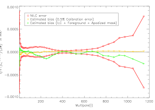
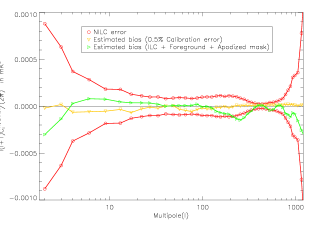
Figure 6: The green right-facing triangles show the bias estimated by implementing the NILC on 50 WMAP-like simulated data. The yellow downward triangles show the estimate of the bias due to calibration error of the order of of $0.5\%$. The red open circles show the total error in the estimate of angular power spectrum using NILC. The top panel uses a linear scale in the horizontal axis, and the bottom panel a logarithmic one.

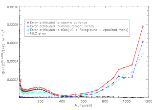
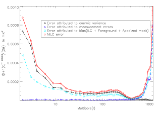
Figure 7: The red circles show the total error in the estimate of the CMB angular power spectrum using the NILC. The black open diamonds show the error due to cosmic variance. The blue upward triangles show the measurement error. The sky blue open squares show the error due to bias uncertainty. The horizontal axis of the top plot is scaled linearly, and that of the bottom plot is scaled logarithmically.

Table 2: Comparison of NILC estimate of binned angular power spectrum (after bias correction) with the estimate of binned angular power spectrum provided by WMAP collaboration.

$l_{b}$	$P_{b,\,\text{NILC}}$	$P_{b,\,\text{WMAP}}$	$P^{\text{ERR}}_{b,\,\text{NILC}}$	$P^{\text{ERR}}_{b,\,\text{WMAP}}$
	$(mK^{2})$	$(mK^{2})$	$(mK^{2})$	$(mK^{2})$
2	4.033e-04	2.009e-04	8.807e-04	9.291e-04
3	5.547e-04	1.051e-03	6.319e-04	7.308e-04
4	7.754e-04	1.105e-03	3.710e-04	3.949e-04
6	6.380e-04	1.022e-03	2.843e-04	3.039e-04
9	7.523e-04	7.432e-04	1.831e-04	1.715e-04
13	6.391e-04	7.906e-04	1.795e-04	1.693e-04
17	8.995e-04	8.396e-04	1.285e-04	1.193e-04
22	6.469e-04	6.922e-04	1.107e-04	1.128e-04
27	9.119e-04	9.915e-04	9.843e-05	1.004e-04
33	1.085e-03	1.146e-03	9.975e-05	9.997e-05
40	1.394e-03	1.468e-03	8.158e-05	8.780e-05
48	1.355e-03	1.379e-03	8.772e-05	9.041e-05
56	1.548e-03	1.536e-03	9.239e-05	9.395e-05
65	1.748e-03	1.784e-03	8.884e-05	8.840e-05
76	1.961e-03	1.977e-03	8.277e-05	8.999e-05
87	2.329e-03	2.382e-03	8.794e-05	9.679e-05
98	2.610e-03	2.628e-03	9.761e-05	1.002e-04
111	3.159e-03	3.128e-03	9.954e-05	1.046e-04
125	3.483e-03	3.535e-03	9.936e-05	1.063e-04
140	4.188e-03	4.278e-03	1.094e-04	1.153e-04
155	4.578e-03	4.558e-03	1.135e-04	1.195e-04
172	5.043e-03	4.989e-03	1.048e-04	1.187e-04
191	5.524e-03	5.560e-03	1.124e-04	1.190e-04
210	5.739e-03	5.768e-03	1.074e-04	1.157e-04
231	5.754e-03	5.750e-03	1.007e-04	1.085e-04
253	5.402e-03	5.383e-03	8.588e-05	9.294e-05
278	4.864e-03	4.843e-03	7.407e-05	7.856e-05
304	3.949e-03	3.943e-03	5.446e-05	6.153e-05
332	3.007e-03	3.050e-03	4.148e-05	4.507e-05
363	2.256e-03	2.275e-03	3.179e-05	3.374e-05
397	1.775e-03	1.792e-03	2.620e-05	2.785e-05
436	1.826e-03	1.828e-03	2.476e-05	2.863e-05
479	2.300e-03	2.319e-03	2.983e-05	3.404e-05
526	2.535e-03	2.533e-03	3.979e-05	4.099e-05
575	2.390e-03	2.451e-03	4.292e-05	4.647e-05
625	2.008e-03	2.011e-03	5.195e-05	5.202e-05
675	1.667e-03	1.757e-03	6.714e-05	6.344e-05
725	2.058e-03	2.012e-03	8.267e-05	8.385e-05
775	2.394e-03	2.271e-03	1.257e-04	1.123e-04
825	2.516e-03	2.594e-03	1.712e-04	1.477e-04
875	2.237e-03	2.277e-03	2.137e-04	1.908e-04
925	2.087e-03	2.051e-03	3.075e-04	2.446e-04
975	1.345e-03	1.333e-03	3.286e-04	3.158e-04
1050	8.890e-04	9.932e-04	3.588e-04	3.425e-04
1150	1.846e-03	9.924e-04	7.788e-04	6.132e-04

4.5 Impact of calibration errors

Calibration errors are a serious issue for precise separation of the CMB from foregrounds using any type of ILC. As discussed by Dick et al. (2010), they ‘conspire’ with the ILC filter to cancel out the CMB. This effect is particularly strong in the high signal to noise ratio regime, which is the case in our present analysis, in particular on large scales. We investigate the impact of this calibration bias by redoing the analysis using slightly modified calibration coefficients (differences of the order of $0.5\%$), and computing the difference between the CMB spectra estimated in both cases. The result, plotted in figure 6, shows that here even at large angular scale, the bias due to calibration error is small. We hence neglect this effect in our estimate of errors on $C_{\ell}$. Note however that this calibration bias will be a concern for those experiments which measure CMB with higher signal to noise ratio than WMAP.

4.6 Impact of beam uncertainties

The uncertainty on beam shapes is equivalent to a calibration error which depends on the harmonic mode $l$. As this uncertainty is essentially at high $l$, where the signal to noise ratio is worse than on large scales, the bias, for small beam shape errors, is not expected to impact much the CMB reconstruction here, and is also neglected in the present analysis.

5 Discussion

5.1 Low power on large scales?

The temperature power spectrum we obtain seems to be, on large scales, systematically lower than the theoretical ‘best fit’ power spectrum (for $\ell<15$) and the WMAP measurement (for $\ell<40$, except for the quadrupole, see figure 4, bottom left panel, and table 3).

Considering that error bars on these scales are cosmic variance dominated, the difference between the power spectrum measured by WMAP and by us from the same original data set is problematic, and deserves a discussion and additional investigation. A systematic shift in the estimated power spectrum at all $l$ below 40 is bound to impact the interpretation of the observations, and the inferred values and limits for cosmological parameters. In the following, we investigate various possible origins for the discrepancy.

Table 3: Difference between the NILC estimate of binned angular power spectrum and the angular power spectrum provided by the WMAP collaboration. Except for the quadrupole, for which our estimate is larger (after debiasing) and except the bins centred at $l=9$ and $l=27$, our estimated power spectrum is lower than the WMAP one.

$l_{b}$	$P_{b,\,\text{NILC}}-P_{b,\,\text{WMAP}}$ $(mK^{2})$
2	2.024e-04
3	-4.963e-04
4	-3.296e-04
6	-3.840e-04
9	0.091e-04
13	-1.515e-04
17	0.599e-04
22	-0.453e-04
27	-0.796e-04
33	-0.610e-04
40	-0.740e-04

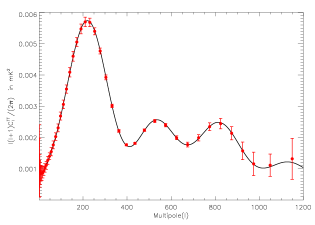
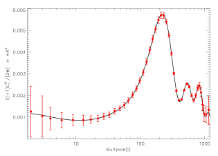
Figure 8: The red filled circles show the average estimated angular power spectrum using NILC from WMAP $7$-year-like simulations. The black solid line show the theoretical angular power spectrum for WMAP best-fit $\Lambda$CDM model. The top panel uses a linear scale in the horizontal axis, and the bottom panel a logarithmic one.

5.1.1 Bias due to the method of spectrum estimation?

Our method is based on the computation of the needlet transform of a masked sky. We check that the method itself is not biased, by computing in the exact same way the power spectrum of 100 pure CMB maps, randomly generated using different seeds. The average estimated power spectrum is computed, and individual recovered power spectra for the 100 realisations visually inspected. We find no evidence of a bias in our power spectrum estimate.

5.1.2 Bias due to the complete analysis chain?

At a next level, we check whether our complete data processing method can generate a bias. We generate two times 50 simulations of the NILC maps for the 7 independent years. The first 50 coincide with the simulations used to estimate an average ILC bias (green curve in figure 6) and correct for it in the real data (the effect is small). The other 50 simulations are used as test data, for which we implement our complete analysis pipeline exactly as done on the WMAP data. For each of them, in particular, we de-bias the resulting power spectrum using the average bias in the first 50 simulations, in the exact same way as was done on the real data.

Figure 8 shows the average angular power spectrum (after bias correction) of CMB temperature anisotropies on these test data sets. The power spectrum matches extremely well the theoretical input angular power spectrum, and does not show any lack of power at large angular scale. This demonstrates that our method does not generate biases by itself. Nor the needlet ILC, nor the way we implement our power spectrum estimation can be responsible for a bias – assuming our data model is right.

We note that the bias correction at $l=2$ is of more than $3\times 10^{-4}$ mK², and that the error on the estimate of this bias is itself of order $5\times 10^{-4}$ mK². This can explain the difference between the WMAP measured quadrupole, and our estimate.

5.1.3 Are simulations representative?

The representativeness of the simulated data sets is of course a major concern. For instance, if our simulated maps had exceedingly large galactic foregrounds, the average bias on the simulations due to residual foregrounds would be too large, and subtracting this residual from the real data would result in an over-correction, and hence a negative bias.

Although significant effort has been put to generate sky simulations as realistic as possible, such a bias due to modelling errors cannot be fully ruled-out (the modelling uncertainty is not easily estimated). For this reason, we look for confirmation using other CMB maps and different analyses.

5.1.4 Confirmation using other WMAP CMB maps?

We have also estimated the power spectrum of WMAP maps directly using the original V and W frequency channel maps, the foreground-reduced V and W channel maps published by the WMAP collaboration, and the WMAP ILC map itself, applying different galactic masks. These estimates also result in low $\ell$ CMB multipoles. In figure 9 we compare the multipoles computed directly on the 7-year NILC map and on the 7-year WMAP ILC. They are almost indistinguishable at low $l$. The very low value of the spectrum of the difference between those two maps shows that the difference between our present power spectrum and the published WMAP spectrum is not due to significant differences in the large scale modes of the maps themselves, but on the power spectrum estimation method (including debiasing).

Power spectra computed directly from the 7-year V and W channels also tend to be lower than the WMAP theoretical best fit. A fraction of the deficit in power on the largest scales ($l=2$ to $l=4$) is due to the mask (there is no bias correction here, except for a global $f_{\rm sky}$ factor). In most of the measured multipoles for $l<30$, there seems to be less power in the maps than theoretically predicted. This is particularly true for conservative masks ($M_{20^{\circ},20^{\circ}}$ and kp2). We note that the power in the V band map decreases with increasing galactic cut. For the $M_{20^{\circ},20^{\circ}}$ mask, the spectra of all maps (Needlet ILC, WMAP ILC, V band and W band) are almost indistinguishable, and on average significantly lower than the theoretical best fit, for $5<l<25$.

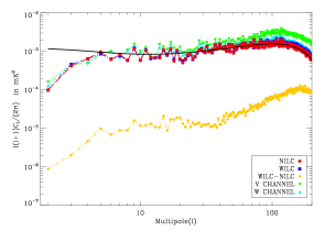
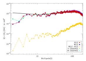
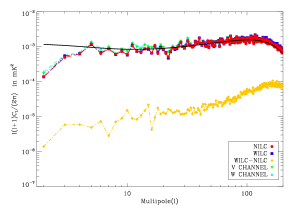
Figure 9: CMB power spectra obtained from different WMAP maps. The red circles show the angular power spectrum obtained by direct calculation of the spectrum of the NILC CMB obtained on WMAP-7year band average maps, masked with an apodised Galactic mask. The mask used is $M_{10^{\circ},10^{\circ}}$ (same mask as used in our analysis) for the top panel, $M_{20^{\circ},20^{\circ}}$ for the middle panel, and kp2 (including point sources) for the bottom panel. The 7-year NILC map power spectrum is fully consistent with the power spectrum of the WMAP 7-year ILC map (blue squares), masked in the same way. No correction for the ILC bias (which depends on the mask used) was applied here. The yellow diamonds show the angular power spectrum of the difference of the two ILC maps. This difference, very low on large scales, rises at higher $l$ because of the larger noise residuals in the WMAP ILC map. The downward and upward triangles show the power spectra of the 7-year V and W channels respectively. As can be seen by comparing the various panels, galactic foregrounds contaminate significantly the V channel at galactic latitudes between 10 and 20 degrees (and, to a lesser extent, the W channel as well). Note also that the lowest multipoles depend somewhat on the exact mask used, as expected for ‘pseudo’ spectra.

5.2 Comparison with other work

We have not been able to identify a source of bias in our analysis which would explain this difference between our power spectrum and the one published by the WMAP collaboration. A significant amount of connected work has been done by various authors to extract a CMB map, and compute CMB power spectra from WMAP data, with different techniques. We now discuss how our present work differs from such previous analyses with similar objectives, and compare the results obtained with various methods and on various WMAP data releases (in particular on large scales).

Delabrouille et al. (2009) make a CMB map from WMAP 5 year data on needlet (spherical wavelet) domains. Our present work is an extension implemented on WMAP $7$-year data. As an additional analysis step, we also use the corresponding NILC weights to obtain clean CMB maps from $7$ individual years, and compute cross spectra to estimate the CMB power spectrum.

A CMB power spectrum has been published with each of the various WMAP data releases (Hinshaw et al., 2003, 2007; Nolta et al., 2009; Larson et al., 2011). The CMB power spectrum on large scale is unexpectedly low in the analysis of the first year data. In subsequent releases, only the quadrupole remains significantly lower than the WMAP best fit model spectrum.

The most recent temperature power spectrum produced by the WMAP collaboration is obtained on the basis of two different techniques for large and small scales. For $\ell\leq 32$, the spectrum is obtained using a Blackwell-Rao estimator applied to a chain of Gibbs samples based on the seven-year ILC map masked with the KQ85y7 mask, which cuts 21.7 % of the sky close to the galactic plane. The difference in power spectrum at low multipoles between this estimate and ours must originate from either the exact way the power spectrum is estimated on large scales (including debiasing), but we do not know at present whether the observed difference is to be expected on the basis of differences in the analysis pipeline, nor its exact significance, as this requires checking details of both analyses, some of which are not available to us at present.

Among the differences, we note that our sky model is based on 4 galactic components (synchrotron, free-free, spinning dust and thermal dust), with spectral indices varying over the sky for synchrotron and thermal dust, while the WMAP 3-year analysis, for instance, uses a three-component model of sky emission. It is possible that a bias correction based on simulations with a 3-component ISM emission yields a higher $C_{l}$ estimate than with a 4-component one. If the origin of the discrepancy is there, it emphasises the need for complete models of sky emission, in which the complexity of the sky can be varied at the level of present modelling uncertainties.

Another particularity of our analysis is the use of cross spectra between data from different years of observations, which in principle makes our analysis impervious to large scale residuals of low frequency noise correlated between the various WMAP channels. Such hypothetical residuals, however, are unlikely to be the main reason for the low-$l$ discrepancy, as demonstrated by the comparison of the 7 year NILC map and the WMAP ILC map at low $l$.

At higher multipoles, the WMAP spectrum is estimated on the seven-year, template-cleaned V- and W-band maps, using (pseudo) cross-spectra between maps obtained for individual differencing assemblies and individual years. Above $\ell=600$, the maps are inverse-noise weighted to reduce the noise variance in the final power spectrum estimate. The WMAP power spectrum is in good agreement with our estimate.

In addition to the analyses published by the WMAP collaboration, the CMB power spectrum inferred from WMAP data sets has been investigated by a number of authors.

Eriksen et al. (2007), in particular, partly re-analyse WMAP 3-year data sets with different methods. They find large scale power spectra systematically lower than the WMAP best fit and published power spectrum, although not as low as our present result for $3\leq l\leq 6$. All the estimated spectra they publish are somewhat different, a feature they interpret, on the basis of differences when the galactic mask is extended, as plausibly due to contamination by residual galactic foreground emission.

On the foreground cleaning side, CMB reconstruction using ILC methods has been performed by several authors. Saha et al. (2008) have implemented an ILC on WMAP 1-year and 3-year data in the harmonic domain. The primary goal of their work is to compute the CMB power spectrum, rather than producing a clean CMB map. They also analyse the bias produced at low $l$ by the ILC in the measured power spectrum. This bias is estimated in the case of an implementation in the harmonic domain, and an equivalent bias correction is made in our case on the basis of Monte-Carlo simulations. In their analysis, Saha et al. (2008) also find, as we do in our present analysis, that both the quadrupole and the octupole are significantly lower than the WMAP best fit.

Samal et al. (2010) estimate CMB polarisation and temperature power spectra using linear combination of WMAP 5 year maps. The authors use different combinations of individual WMAP differencing assemblies, rather than different years, to compute independent sky maps, but find, again, somewhat lower CMB power on large scale than both the WMAP estimate and best fit.

Hence, significant differences between the low CMB multipoles are found by different authors, using different methods. All the analyses are based on the same sky emission, and hence should agree to up to errors which exclude cosmic variance. Even worse, these analyses sometimes start from the same original data, so that even the instrumental noise errors should be the same. This demonstrates that the low $l$ power spectrum estimation is sensitive to details of the analysis pipeline. The exact origin of the discrepancy between the various estimates remains to be understood, but the fact that there still is debate on the exact value of the low $l$ CMB multipoles is a concern, which illustrates the difficulty of component separation and power spectrum estimation on large scales. Solving these issues is important for the tentative measurement of primordial tensor modes with Planck and with future CMB polarisation experiments such as the recently proposed CMBPol, EPIC, and COrE space missions (Baumann et al., 2009; Bock et al., 2008; The COrE Collaboration et al., 2011).

6 Conclusion

The precise measurement of cosmological parameters has set a new goal in the effort to estimate the angular power spectrum of the CMB by present and future CMB experiments. This effort is primarily boosted by the ever increasing improvement in the sensitivity and resolution of the CMB observations. However, the removal of foreground contamination from the observed sky maps is a mandatory preliminary step for the accurate estimation of angular power spectrum.

In this paper, we have described a new methodology to estimate the angular power spectrum of CMB temperature anisotropy from WMAP 7-year data. We have used linear combination of sky maps decomposed on a frame of spherical wavelets (needlets), to construct a map of CMB anisotropies with low contamination from foreground signals and instrumental noise. The CMB temperature anisotropy map has been estimated by implementing the NILC on WMAP $7$-year band average maps at the highest resolution (with HEALPix pixelisation parameter nside equal to $1024$). We have included, in our analysis, three foreground templates in the set of analysed observations for better performance of our component separation. Our method for CMB cleaning does not rely strongly upon any assumed model of foreground emission and detector noise properties, and hence, is not very sensitive to the uncertainty and insufficiency in foreground and noise modelling. However, the cleaned CMB map always contains, at some level, non-vanishing residual foreground and residual noise, superimposed on actual CMB signal.

To minimise the impact of uncertainties in detector noise levels and correlation between channels, the angular power spectrum of the CMB has been estimated from all possible (twenty one in our case) cross power spectra of clean CMB maps for $7$ individual years of observations with independent noise. The estimates of CMB maps for the $7$ individual years are obtained by using the NILC weights obtained by implementing a needlet ILC on WMAP $7$-year band average maps.

To reduce the impact of foreground signals on the measured CMB power spectrum, in addition to using low foreground linear combinations of input WMAP channels and of ancillary data, we have applied the point source mask provided by the WMAP collaboration, and then filled the masked regions by a interpolation procedure. We have also used an apodised symmetric mask to lower the impact of residuals emission from the interstellar medium in our analysis.

Biases due to random correlation of the CMB with the ISM in our NILC pipeline have been estimated using $50$ realisations of WMAP-like simulations. These biases turn out to be smaller than the other sources of error on most of the range of $l$, but not completely negligible, so we use the average bias measured on these 50 simulations to de-bias our estimate on WMAP data. We find that our de-biased angular power spectrum agrees well with the estimate of angular power spectrum provided by the WMAP collaboration, except at large angular scale, where our estimate seems to be systematically lower, but where the fundamental uncertainties are high. A number of tests, performed on simulated data sets, using different approaches to power spectrum estimation on WMAP data, confirm that the released WMAP maps seems to contain somewhat less CMB anisotropies on large scales than expected from the WMAP best fit model (marginally within cosmic variance errors, as can be seen in the bottom panel of figure 5). This still has to be elucidated.

The error bars in our estimate of de-biased angular power spectrum have been computed very carefully. They comprise estimates of the measurement and cosmic variance error on the basis of the internal scatter of 21 independent cross-spectra, and of the error in the estimate of the ILC bias. Errors due to miscalibration or to imperfect beam knowledge have been shown to be small enough to be negligible, considering the calibration uncertainty estimates provided by the WMAP collaboration. Our total error bars are comparable to the error in the estimate of angular power spectrum provided by the WMAP collaboration. As the measurement errors are estimated from the internal scatter of independent cross spectra for each bin in $l$, they do not rely on a model of WMAP detector noise.

The fact that there still is not a convincing consensus in the scientific community on the exact value of the low $l$ CMB multipoles is a concern, which demonstrates the difficulty of extracting precisely the CMB emission from galactic foregrounds on large scales.

References

- Atrio-Barandela et al. (2008) Atrio-Barandela, F., Kashlinsky, A., Kocevski, D., & Ebeling, H. 2008, ApJ, 675, L57
- Baumann et al. (2009) Baumann, D., Cooray, A., Dodelson, S., Dunkley, J., Fraisse, A. A., Jackson, M. G., Kogut, A., Krauss, L. M., Smith, K. M., & Zaldarriaga, M. 2009, in American Institute of Physics Conference Series, Vol. 1141, American Institute of Physics Conference Series, ed. S. Dodelson, D. Baumann, A. Cooray, J. Dunkley, A. Fraisse, M. G. Jackson, A. Kogut, L. Krauss, M. Zaldarriaga, & K. Smith , 3–9
- Betoule et al. (2009) Betoule, M., Pierpaoli, E., Delabrouille, J., Le Jeune, M., & Cardoso, J. 2009, A&A, 503, 691
- Bock et al. (2008) Bock, J., Cooray, A., Hanany, S., Keating, B., Lee, A., Matsumura, T., Milligan, M., Ponthieu, N., Renbarger, T., & Tran, H. 2008, ArXiv e-prints
- Bonaldi et al. (2007) Bonaldi, A., Ricciardi, S., Leach, S., Stivoli, F., Baccigalupi, C., & de Zotti, G. 2007, MNRAS, 382, 1791
- Bottino et al. (2008) Bottino, M., Banday, A. J., & Maino, D. 2008, MNRAS, 389, 1190
- Bottino et al. (2010) —. 2010, MNRAS, 402, 207
- Condon et al. (1998) Condon, J. J., Cotton, W. D., Greisen, E. W., Yin, Q. F., Perley, R. A., Taylor, G. B., & Broderick, J. J. 1998, AJ, 115, 1693
- Delabrouille & Cardoso (2009) Delabrouille, J. & Cardoso, J. 2009, in Lecture Notes in Physics, Berlin Springer Verlag, Vol. 665, Data Analysis in Cosmology, ed. V. J. Martínez, E. Saar, E. Martínez-González, & M.-J. Pons-Bordería, 159–205