Gravipulsons

Abstract

We search for self-gravitating oscillating field lumps (pulsons) in the scalar model with logarithmic potential. With the use of a Krylov-Bogoliubov-type asymptotic expansion in the gravitational constant, the pulson solutions of the Einstein-Klein-Gordon system are obtained in the Schwarzschild coordinates. They are expressed in terms of solutions of the singular Hill’s equation. The masses of the obtained pulsons are calculated. The initial conditions are found under which the pulson solutions become periodic. These conditions are then used in direct numerical integration of the Einstein-Klein-Gordon system. It is shown that they do evolve into a very long-lived periodic pulson. Stability of the self-gravitating pulsons and their possible astrophysical applications are briefly discussed.

I Introduction

A large number of modern astrophysical observations suggest the existence of scalar fields in our Universe as possible candidates for dark matter. Pulsons are localized configurations of the fields having oscillating energy density. Numerical simulations of Seidel and Suen Seidel and Suen (1991); *Seidel-Suen2 have revealed the existence of long-lived self-gravitating pulsons, so-called oscillating soliton stars or oscillatons, in the Einstein-Klein-Gordon (EKG) system

$$R_{\mu\nu}-\frac{1}{2}Rg_{\mu\nu} = \varkappa\left[\phi_{,\mu}\phi_{,\nu}-\left(\frac{1}{2}\phi_{,\alpha}\phi^{,\alpha}-U(\phi)\right)g_{\mu\nu}\right],$$

$$\phi_{;\alpha}^{;\alpha}+U^{\prime}(\phi) = 0$$ (1)

with the potential $U(\phi)=(m^{2}/2)\phi^{2}$ corresponding to a free massive scalar field. The authors have established that soliton stars can be formed from rather general initial field distributions due to specific relaxation process, the gravitational cooling.

Pulsons were first observed numerically by Bogolubsky and Makhankov Bogolubsky and Makhankov (1976); *Bog-Makh2 in the Klein-Gordon (KG) model with $\phi^{4}$ and $sG$ potentials. In these cases, in the absence of gravity, the formation of the pulsons occurs solely due to self-coupling effects. In the present-day literature such configurations are often called oscillons, but below we shall use their original name, pulsons Bogolubsky (1976).

Subsequent investigations have shown that pulsons exist in various models and spatial dimensions, and that they evolve from the diversity of initial conditions Marques and Ventura (1977); Bogolubsky (1979); Olsen and Samuelsen (1981); Geicke (1984); Maslov (1990); Gleiser (1994); Copeland et al. (1995); Maslov and Shagalov (1997); Piette and Zakrzewski (1998); Hormuzdiar and Hsu (1999); Maslov and Shagalov (2001); Dymnikova et al. (2000); Honda and Choptuik (2002); Ureña-Lópes (2002); Gleiser and Howell (2003); Kasuya et al. (2003); Koutvitsky and Maslov (2005, 2006); Gleiser and Sicilia (2009) (see Fodor et al. (2008) for a review). It turns out that pulsons can arise from both uniform and non-uniform field distributions. Thus pulsons can emerge in scalar condensates due to the parametric instability of the spatially uniform background oscillating near a vacuum value Maslov and Shagalov (2001); Gleiser and Howell (2003); Kasuya et al. (2003); Koutvitsky and Maslov (2006). In this case the energy of the background oscillations is transferred to an incipient pulson via the resonance mechanism. Quite a different scenario is realized when pulsons are formed from localized field distributions that appear, e.g., in shrinking cylindrical domain walls Geicke (1984), in collapsing spherical bubbles Gleiser (1994); Copeland et al. (1995), or at bubble collisions Dymnikova et al. (2000). In such a case an initial field lump sheds excessive energy by radiation of scalar waves (gravitational cooling of the soliton stars) and settles into a quasi-stable state, the pulson, whose lifetime depends strongly on the initial conditions. This suggests the existence of such initial conditions that evolve into very long-lived quasi-periodic, or even infinitely long-lived periodic pulsons. The latter would imply the existence of exact localized time-periodic solutions. For the $\phi^{4}$, $\phi^{3}-\phi^{4}$, and $sG$ models, certain of these initial configurations have been found numerically in Copeland et al. (1995); Piette and Zakrzewski (1998); Hormuzdiar and Hsu (1999); Honda and Choptuik (2002). Recently, in Ref. Fodor et al. (2010) small amplitude pulson solutions of the EKG system have been obtained for the potentials expansible in a power series. This brings up the following question: How does gravity affect the dynamics of the finite amplitude pulsons? For example, could gravity turn non-periodic pulson solutions into periodic ones? Consideration of finite amplitude pulsons takes on great significance in the case where a scalar field potential is not expansible in a power series in the small amplitude limit.

In this paper we search for pulsons in the EKG system (1) with the potential

$$U(\phi)=\frac{m^{2}}{2}\phi^{2}\left(1-\ln\frac{\phi^{2}}{\sigma^{2}}\right),$$ (2)

where $\phi$ is a real scalar field, $m$ is a bare mass (in units $\hbar=c=1$), and $\sigma$ is a characteristic amplitude of the field which is assumed to be finite, but not too large, so that $\varkappa\sigma^{2}\ll 1$, where $\varkappa$ is the gravitational constant.

The nonlinear KG equation with the logarithmic potential (2) was first considered in quantum field theory by Rosen Rosen (1969) and later by Bialynicki-Birula and Mycielski Bialynicki-Birula and Mycielski (1975). In general, for the nonlinear KG equation the potential (2) is the only one which permits real solutions of the form $\phi=a(t)u(\mathbf{r})$ to exist Maslov (1990). Such singular potentials currently appear in inflationary cosmology Barrow and Parsons (1995) and in some supersymmetric extensions of the standard model (flat direction potentials in the gravity mediated supersymmetric breaking scenario) Enqvist and McDonald (1998). The logarithmic term in parentheses arises due to quantum corrections to the bare inflaton mass.

The paper is organized as follows. In Sec. II, using the smallness of the gravitational constant, we obtain the approximate solution of the EKG system (1) which describes time-periodic pulsons of a finite amplitude in the Schwarzschild metric $ds^{2}=Bdt^{2}-Adr^{2}-r^{2}(d\vartheta^{2}+\sin^{2}\vartheta\;d\varphi^{2})$. In Sec. III we use the obtained solution to find the initial conditions for direct numerical integration of the system. We show that these initial conditions do evolve into a very long-lived periodic pulson. Stability of the self-gravitating pulsons and their possible astrophysical meaning are briefly discussed in Sec. IV.

II Solution

After the scaling $t\rightarrow t/m,\;r\rightarrow r/m,\;\phi/\sigma\rightarrow\phi,$ $\varkappa\sigma^{2}/2\rightarrow\varkappa,$ the system (1) takes the form

$$\frac{A_{r}}{A}+\frac{A-1}{r}=\varkappa r\left(\frac{A}{B}\phi_{t}^{2}+\phi_{r}^{2}+A\phi^{2}(1-\ln\phi^{2})\right),$$ (3)

$$\frac{B_{r}}{B}-\frac{A-1}{r}=\varkappa r\left(\frac{A}{B}\phi_{t}^{2}+\phi_{r}^{2}-A\phi^{2}(1-\ln\phi^{2})\right),$$ (4)

$$\frac{A}{B}\phi_{tt}-\phi_{rr}-\frac{2}{r}\phi_{r}+\left(\frac{A}{2B}\right)_{t}\phi_{t}+\frac{B}{2A}\left(\frac{A}{B}\right)_{r}\phi_{r}=A\phi\ln\phi^{2},$$ (5)

where $\varkappa\ll 1$ is the rescaled gravitational constant. Looking for localized solutions, we impose the boundary conditions $\phi(t,\infty)=0,\;A(t,\infty)=1,\;B(t,\infty)=1,\;\phi_{r}(t,0)=0,\;A(t,0)=1.$

If we set $\varkappa=0$, from (3)-(5) we immediately obtain $A=B=1$ and arrive at the nonlinear Klein-Gordon equation

$$\phi_{tt}-\phi_{rr}-(2/r)\phi_{r}-\phi\ln\phi^{2}=0.$$ (6)

This equation has a whole family of exact pulson solutions Marques and Ventura (1977); Bogolubsky (1979); Maslov (1990). The simplest of them is given by

$$\phi(t,r)=a(t)e^{(3-r^{2})/2},$$ (7)

where $a(t)$ satisfies the equation of a nonlinear oscillator,

$$a_{tt}=-dV(a)/da,\quad V(a)=(a^{2}/2)(1-\ln a^{2}).$$ (8)

As is clear from the shape of the potential $V(a)$ depicted in Fig. 1, oscillations are possible in the range $-1<a(t)<1$, so we shall consider below that the pulson’s amplitude may be finite, $\left|\phi\right|\lesssim O(1)$.

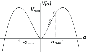
Figure 1: The shape of the potential $V(a)$. Initial conditions for the nonlinear oscillator (8) are $a(0)=a_{max},\ a_{t}(0)=0$.

For small $\varkappa\ll 1$ we construct the Krylov-Bogoliubov-type asymptotic expansion (see, e.g., Nayfeh (1973)) near the non-gravitating pulson,

$$\phi(t,r) = \left[a(\theta)+\varkappa Q(\theta,r)+O(\varkappa^{2})\right]e^{(3-r^{2})/2},$$ (9)

$$\theta_{t} = 1+\varkappa\Omega+O(\varkappa^{2}),$$ (10)

where $a(\theta)$ satisfies Eqs. (8), with the phase $\theta$ instead of $t$, and the initial conditions $a(0)=a_{\max}<1$, $a_{\theta}(0)=0$. The function $Q(\theta,r)$ and the constant $\Omega$ to be found describe the deviation of the pulson’s shape from the Gaussian one and the frequency shift $\delta\omega/\omega=\varkappa\Omega$ due to gravitational effects.

Setting in Eqs. (3), (4)

$$A(t,r)=(1-r_{g}/r)^{-1},\quad B(t,r)=(1-r_{g}/r)e^{-s}$$ (11)

and using (9), (10), we find

$$r_{g}(t,r) = \varkappa\int_{0}^{r}\left(\frac{1}{B}\phi_{t}^{2}+\frac{1}{A}\phi_{r}^{2}+\phi^{2}(1-\ln\phi^{2})\right)r^{2}dr$$ (12)

$$= \varkappa\left[V_{\max}\left((\sqrt{\pi}/2)e^{r^{2}}\mathrm{erf}\,r-r\right)-a^{2}r^{3}\right]e^{3-r^{2}}$$

$$+O(\varkappa^{2}),$$

$$s(t,r) = 2\varkappa\int_{r}^{\infty}\left(\frac{A}{B}\phi_{t}^{2}+\phi_{r}^{2}\right)r\,dr$$ (13)

$$= \varkappa\left(2V_{\max}+a^{2}\ln a^{2}+a^{2}r^{2}\right)e^{3-r^{2}}$$

$$+O(\varkappa^{2}),$$

where $a=a(\theta(t))$, $V_{\max}=V(a_{\max})$. Substituting (9) into (5) leads to the equation for $Q(\theta,r)$:

$$Q_{\theta\theta}-Q_{rr}+(2/r)(r^{2}-1)Q_{r}-(2+\ln a^{2})Q=S(a,r),$$ (14)

where

$$S(a,r) = a\{V_{\max}[\sqrt{\pi}(2-r^{2}-\ln a^{2})(2r)^{-1}e^{r^{2}}\mathrm{erf}\,r$$ (15)

$$+\,3r^{2}-4-3\ln a^{2}]-5a^{2}r^{2}+2a^{2}r^{4}$$

$$+\,a^{2}-2a^{2}\ln^{2}a^{2}\}e^{3-r^{2}}-2\Omega a\ln a^{2}.$$

Its solution is given by

$$Q(\theta,r)=\frac{1}{r}\sum_{n=0}^{\infty}c_{n}X_{n}(\theta)H_{2n+1}(r),$$ (16)

where $c_{n}=\pi^{-1/4}\left[2^{2n+1}\left(2n+1\right)!\right]^{-1/2}$, and $H_{2n+1}(r)$ are Hermite polynomials. The functions $X_{n}(\theta)$ must satisfy the non-homogeneous singular Hill’s equation

$$X_{n_{\,\scriptstyle{\theta\theta}}}+\left(E-2-\ln a^{2}\right)X_{n}=f_{n}(a),$$ (17)

where $E=E_{n}=4n$,

$$f_{n}(a)=2c_{n}\int_{0}^{\infty}S(a,r)H_{2n+1}(r)e^{-r^{2}}r\,dr.$$ (18)

The calculation gives

$$f_{0}(a) = D_{0}(a)-\sqrt{2}\pi^{1/4}\Omega a\ln a^{2},$$ (19)

$$f_{n}(a) = D_{n}(a)\quad(n=1,2,...),$$ (20)

$$D_{n}(a) = \frac{(-1)^{n}(2n)!c_{n}}{2^{n+4}(2n-1)n!}\sqrt{\frac{\pi}{2}}e^{3}$$ (21)

$$\times\{a^{3}(4n^{2}-1)(4n^{2}-4n-7-16\ln^{2}a^{2})$$

$$-2V_{\max}a[24n^{3}+20n^{2}-46n-1$$

$$+4(2n-1)(6n+5)\ln a^{2}]\}.$$

Note that $f_{n}(a)$ is a $T$-periodic function of $\theta$, while $\ln a^{2}$ on the left hand side of Eq. (17) is a $T/2$-periodic one, where $T$ is a period of $a(\theta)$.

Solutions of the homogeneous singular Hill’s equation were investigated in Ref. Koutvitsky and Maslov (2006). In accordance with the Floquet theory (see, e.g., Whittaker and Watson (1927)) Eq. (17) with $f_{n}=0$ has two linearly independent solutions of the form $\varphi(\theta)e^{\mu\theta}$ and $\varphi(-\theta)e^{-\mu\theta}$, where $\mu$ is a characteristic exponent, and $\varphi(\theta)$ is a $T$-periodic ($T/2$-periodic or $T/2$-antiperiodic) function. Obviously, we can set $\varphi(0)=1$. Let $X^{\pm}\left(\theta\right)$ be two solutions of the homogenious Eq. (17) (with $f_{n}=0$) satisfying the conditions $X^{+}\left(0\right)=1$, $X_{{}_{\,\scriptstyle{\theta}}}^{+}\left(0\right)=0$, $X^{-}\left(0\right)=0$, $X_{{}_{\,\scriptstyle{\theta}}}^{-}\left(0\right)=1$. They can be written as

$$X^{+}\left(\theta\right) = \frac{1}{2}\left[\varphi(\theta)e^{\mu\theta}+\varphi(-\theta)e^{-\mu\theta}\right],$$ (22)

$$X^{-}\left(\theta\right) = \frac{1}{2\left(\mu+\varphi_{{}_{\,\scriptstyle{\theta}}}(0)\right)}\left[\varphi(\theta)e^{\mu\theta}-\varphi(-\theta)e^{-\mu\theta}\right].$$ (23)

If $\left|X^{+}\left(T/2\right)\right|>1$, we have the resonance case: $\mu>0$ and is determined by the equation $\cosh(\mu T/2)=\left|X^{+}\left(T/2\right)\right|$, $\varphi(\theta)$ is a real $T/2$-periodic or $T/2$-antiperiodic function, and hence oscillations of $X^{\pm}\left(\theta\right)$ grow exponentially with $\theta$. If $\left|X^{+}\left(T/2\right)\right|<1$, we have the non-resonance case: $\mu=i\nu$, and $\varphi(\theta)$ is a complex $T/2$-periodic function such that $\varphi^{\ast}(\theta)=\varphi(-\theta)$. Hence the solutions $X^{\pm}\left(\theta\right)$ are bounded. They can be periodic (with some period), or non-periodic depending on $\nu$, which is determined by $\cos(\nu T/2)=X^{+}\left(T/2\right)$. These cases are realized in different domains of the $(E,a_{\max}^{2})$ plane that make up a stability-instability chart. The domains with $\mu>0$ are known as resonance zones. The special case $\left|X^{+}\left(T/2\right)\right|=1$ is realized on their boundaries where $\mu=0$. Then one of the solutions, either $X^{+}\left(\theta\right)$ or $X^{-}\left(\theta\right)$, is a $T$-periodic ($T/2$-periodic or $T/2$-antiperiodic) function, and another one is proportional to the product of this function times $\theta$ plus some $T$-periodic function ($T/2$-periodic or $T/2$-antiperiodic, respectively).

The surface $\mu(E,a_{\max}^{2})$ over the resonance zones has been constructed in Ref. Koutvitsky and Maslov (2006). For discrete $E=4n$ the above functions acquire the subscript $n$, so we shall write $\varphi_{n}(\theta)$, $X_{n}^{\pm}\left(\theta\right)$, $\mu_{n}(a_{\max}^{2})$.

Each cross-section of the surface $\mu(E,a_{\max}^{2})$ with the plane $E=4n,\ n=1,2,...$, gives the characteristic exponent $\mu_{n}$ as a function of $a_{\max}^{2}$. This function is represented by a series of peaks $\mu_{n}>0$ separated by intervals of stability. By superposing the curves $\mu_{n}(a_{\max}^{2})$ for all considered modes $n=1,2,...,N$, one gets the pattern shown in Fig. 2. The mode $n=0$ corresponds to the above special case $\mu=0$ and thus does not contribute to the pattern.

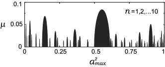
Figure 2: A collection of the resonance peaks obtained by superposition of the functions $\mu_{n}(a_{max}^{2})$.

The obtained composite plot gives an idea of the existence of unstable and (quasi)stable modes in different regions of the $a_{\max}^{2}$ axis and demonstrates the tendency to progressively fill the interval $0<a_{\max}^{2}<1$ by the resonant peaks as the successively higher energy levels $E_{n}=4n$ are accounted for.

In terms of $X_{n}^{\pm}\left(\theta\right)$ the general solution of Eq. (17) is written as

$$X_{n}\left(\theta\right) = \left(X_{n}\left(0\right)-\int_{0}^{\theta}X_{n}^{-}f_{n}\,d\theta\right)X_{n}^{+}\left(\theta\right)$$ (24)

$$+\left(X_{n_{\,\scriptstyle{\theta}}}\left(0\right)+\int_{0}^{\theta}X_{n}^{+}f_{n}\,d\theta\right)X_{n}^{-}\left(\theta\right).$$

The solutions $X_{0}^{\pm}\left(\theta\right)$ have the form

$$X_{0}^{+}\left(\theta\right) = \xi q^{-1/3}(\xi^{2})-\xi_{\theta}\int_{0}^{\theta}K(\xi^{2})\,d\theta,$$ (25)

$$X_{0}^{-}\left(\theta\right) = -(\omega_{0}^{2}-1)^{-1}\xi_{\theta},$$ (26)

where the notations $\xi(\theta)=a/a_{\max}$, $\omega_{0}^{2}=1-\ln a_{\max}^{2}$ are introduced,

$$\xi_{\theta}^{2}=(\omega_{0}^{2}-1)(1-\xi^{2})q^{-2/3}(\xi^{2})$$ (27)

is the first integral of Eq. (8) in terms of $\xi(\theta)$, and the functions $q(\xi^{2})$ and $K(\xi^{2})$ are

$$q(\xi^{2}) = \left(\frac{\omega_{0}^{2}-1}{\omega_{0}^{2}+(1-\xi^{2})^{-1}\xi^{2}\ln\xi^{2}}\right)^{3/2},$$ (28)

$$K(\xi^{2}) = \frac{1-q(\xi^{2})}{1-\xi^{2}}q^{-1/3}(\xi^{2}).$$ (29)

Note that $0<\left(1-\omega_{0}^{-2}\right)^{3/2}\leqslant q(\xi^{2})\leqslant 1$, $dq/d\xi^{2}>0\;(\xi^{2}\leqslant 1)$, and $q(1)=1$. Since $K(\xi^{2})$ is a sign-definite periodic function of $\theta$, its average $\overline{K}=T^{-1}\int_{0}^{T}K\,d\theta\neq 0$, so the solution (25) can be represented in the form $X_{0}^{+}\left(\theta\right)=-\overline{K}\xi_{\theta}\theta+\psi(\theta)$, where $\psi(\theta)$ is a $T/2$-antiperiodic function with $\overline{\psi(\theta)}=0$ [here and elsewhere the bar means the average over the period $T$ of $a(\theta)$]. Thus oscillations of $X_{0}^{+}\left(\theta\right)$ grow linearly with $\theta$ for any $a_{\max}$. This is in agreement with the fact that $X_{0}^{+}\left(T/2\right)=-1$ and the line $E=0$ is the boundary of a resonance zone on the $(E,a_{\max}^{2})$ plane Koutvitsky and Maslov (2006). The equality $X_{0}^{+}\left(T/2\right)=-1$ immediately follows from Eq. (25) if one takes into account that $\xi(T/2)=-1$, $\xi_{\theta}(T/2)=0$ (see Fig. 1).

The requirement of boundedness of the general solution $X_{0}\left(\theta\right)\$(24) determines $\Omega$ and, hence, the frequency shift in accordance with Eq. (10). Indeed, substituting $X_{0}^{+}\left(\theta\right)$, $X_{0}^{-}\left(\theta\right)$, and $f_{0}(a)$ into Eq. (24) and integrating by parts, we find that the linearly growing terms cancel out if

$$\Omega=\frac{\sqrt{2}}{\pi^{1/4}a_{\max}}\left(\frac{\overline{X_{0}^{+}\left(\theta\right)D_{0}(a)}}{\ln a_{\max}^{2}}-X_{0}\left(0\right)\overline{K}\right).$$ (30)

Under the condition (30) the solution $X_{0}\left(\theta\right)$ is a bounded $T$-periodic function.

To obtain the corresponding conditions for $n\geqslant 1$, we substitute (22), (23) into (24) and require that $X_{n}\left(\theta\right)=X_{n}\left(\theta+T\right)$. In this equality the integrals between the limits $0$ and $\theta$ cancel out. The remaining terms make up a linear combination of the independent solutions $\varphi_{n}(\theta)e^{\mu_{n}\theta}$ and $\varphi_{n}(-\theta)e^{-\mu_{n}\theta}$. Equating to zero coefficients of these solutions and using the identities

$$e^{-\mu_{n}T/2}\overline{\varphi_{n}(\theta)e^{\mu_{n}\theta}f_{n}(a)} = e^{\mu_{n}T/2}\overline{\varphi_{n}(-\theta)e^{-\mu_{n}\theta}f_{n}(a)}$$ (31)

$$= \frac{\overline{X_{n}^{+}\left(\theta\right)f_{n}(a)}}{\cosh\left(\mu_{n}T/2\right)},$$

$$\mu_{n}+\varphi_{n_{\,\scriptstyle{\theta}}}(0)=\frac{X_{n_{\,\scriptstyle{\theta}}}^{+}\left(T\right)}{\sinh\left(\mu_{n}T\right)},$$ (32)

we arrive at the conditions

$$X_{n}\left(0\right) = -\frac{T}{X_{n_{\,\scriptstyle{\theta}}}^{+}\left(T\right)}\overline{X_{n}^{+}\left(\theta\right)f_{n}(a)},$$ (33)

$$X_{n_{\,\scriptstyle{\theta}}}\left(0\right) = 0.$$ (34)

Note that $X_{n_{\,\scriptstyle{\theta}}}^{+}\left(T\right)\neq 0$ because $\mu_{n}+\varphi_{n_{\,\scriptstyle{\theta}}}(0)$ in (32) is proportional to the Wronskian $W\left(\varphi_{n}(\theta)e^{\mu_{n}\theta},\ \varphi_{n}(-\theta)e^{-\mu_{n}\theta}\right)$. Equation (32) can be easily derived if one expresses $\varphi_{n}(\theta)$ from (22) in terms of $X_{n}^{+}\left(\theta\right)$ and $X_{n}^{+}\left(\theta+T\right)$ and takes into account that $X_{n}^{+}\left(T\right)=\cosh\left(\mu_{n}T\right)$.

Interestingly, Eq. (33) is still valid on the boundaries of resonance zones, Eq. (34) being no longer necessary. In particular, this is true for $n=0$. Indeed, differentiation of (25) gives $X_{0_{\,\scriptstyle{\theta}}}^{+}\left(T\right)=-T\overline{K}\ln a_{\max}^{2}$. To calculate $\overline{X_{0}^{+}\left(\theta\right)f_{0}(a)}$ we substitute $a\ln a^{2}=a_{\theta\theta}=a_{\max}\ln a_{\max}^{2}X_{0_{\,\scriptstyle{\theta}}}^{-}\left(\theta\right)$ in (19) and, integrating by parts, take into account that $W\left(X_{0}^{+}\left(\theta\right),\ X_{0}^{-}\left(\theta\right)\right)=1$. As a result, we arrive at the condition (30) again.

Thus, under the conditions (30), (33), (34) the solution (16) is $T$-periodic with respect to $\theta$. This means the solution (9) is also periodic [with the period $(1+\varkappa\Omega)^{-1}T$ with respect to $t$]. Note it involves the free parameters $a_{\max}$, $X_{0}\left(0\right)$, and $X_{0\,_{\scriptstyle{\theta}}}(0)$.

To be certain that the obtained solution is correct, we examine the mass conservation law. The mass of a self-gravitating field lump is defined as $M=4\pi\int_{0}^{\infty}T_{0}^{0}r^{2}dr$, where $T_{0}^{0}$ is the energy density of the scalar field involved in the EKG system (1). In terms of the rescaled variables it can be written as $M=(2\pi\sigma^{2}/m)\lim_{r\rightarrow\infty}(r_{g}(t,r)/\varkappa)$, where $r_{g}(t,r)$ is defined in (12), $\varkappa$ being the rescaled gravitational constant. This limit must be time independent. To check this, we substitute the solution (9) into (12) and calculate the limit of $r_{g}/\varkappa$ in the first order in $\varkappa$ using the orthogonality of the Hermite polynomials. The result is given by

$$M = \frac{\left(e\sqrt{\pi}\right)^{3}\sigma^{2}V_{\max}}{m}\Biggl{\{}1-\varkappa\frac{\sqrt{2}a_{\max}}{\pi^{1/4}V_{\max}}\biggl{[}X_{0}\left(0\right)\ln a_{\max}^{2}$$ (35)

$$- \frac{e^{3}\pi^{1/4}}{128}a_{\max}^{3}\left(1+14\ln a_{\max}^{2}\right)\biggr{]}+O(\varkappa^{2})\ \Biggr{\}},$$

which is evidently constant.

Since $\varkappa\ll 1$, the gravitational field created by this mass is weak, as is clearly seen from (11)-(13). In the limit $\varkappa\rightarrow 0$ the gravity vanishes. However, the rescaled scalar field persists, satisfying Eq. (6), and its amplitude may have any value in the range $0<a_{\max}<1$. As $a_{\max}$ changes from unity to zero, the pulson’s frequency changes from zero to infinity, correspondingly. In particular, in the small amplitude limit the pulson’s frequency is $\omega_{0}=\left(1-\ln a_{\max}^{2}\right)^{1/2}$.

Thus, we have obtained a three-parametric family of the spatially localized time-periodic solutions (9)-(13) of the system (3)-(5), wherein only the smallness of the rescaled gravitational constant $\varkappa\;$has been. Note that the smallness of the pulson’s amplitude, $a_{\max}\ll 1,$ is not assumed in the above consideration. To our knowledge, this is the first example of the pulson solutions of the EKG system, that have an arbitrary frequency. We have named them gravipulsons.

III Numerical simulation

Our solution, however, is an approximate one. It was obtained in the first order in the gravitational constant. Hence its deviation from an exact solution increases in time, as happens with any asymptotic solution in the theory of nonlinear oscillations Nayfeh (1973). But we can go back in time and take the initial state of the obtained solution as initial conditions for direct numerical integration of the starting EKG system. As a result, we have a three-parametric family of the initial conditions:

$$\phi(0,r) = a_{\max}e^{(3-r^{2})/2}+\varkappa G(r;a_{\max},X_{0}\left(0\right)),$$ (36)

$$\phi_{t}(0,r) = 2\varkappa c_{0}X_{0\,_{\scriptstyle{\theta}}}(0)e^{(3-r^{2})/2}.$$ (37)

The function $G(r;a_{\max},X_{0}\left(0\right))=Q(0,r)e^{(3-r^{2})/2}$ describes admissible deformations of the initial pulson’s profile which evolve into periodic solutions. In calculating $G$ we assume that $a_{\max}$ belongs to one of the intervals of quasi-stability Koutvitsky and Maslov (2005, 2006) where $X_{n}^{\pm}\left(\theta\right)$, with $1\leqslant n\leqslant N$, are bounded for sufficiently large $N$. This can be easily inspected by numerical integration of the Hill’s equation, taking into account that the boundedness of $X_{n}^{\pm}\left(\theta\right)$ is equivalent to the condition $\left|X_{n}^{+}\left(T/2\right)\right|<1$. We restrict ourselves to the summation from $0$ to $N$ in (16). In deciding on $N$, it is necessary to take into account that the related error in $Q$ must not exceed $O(\varkappa)$. Below we take $\varkappa=0.005$, $N=9$, and set $X_{0}\left(0\right)=X_{0\,_{\scriptstyle{\theta}}}(0)=0$ for simplicity.

Figure 3 shows the examples of the admissible deformations calculated for three different values of $a_{\max}$.

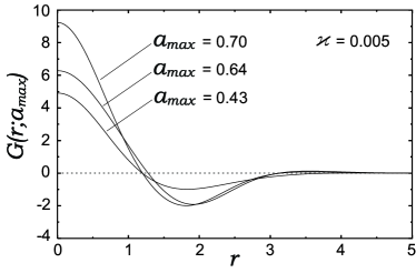
Figure 3: Admissible deformations of the initial pulson’s profile calculated by formula (16) with $X_{0}(0)=0$ and $X_{n}(0)$ (33).

In Figs. 4 and 5 we compare our solution (9)-(13) (solid lines) with the results of direct numerical integration of the EKG system (indicated by dots). We started with one of the admissible deformations of the pulson’s profile that we have found (see Fig. 3). Oscillations of the scalar field and metric at the center of the pulson are shown in Fig.  4. Figure 5 shows the pulson’s and metric’s profiles taken in some intermediate moment of time.

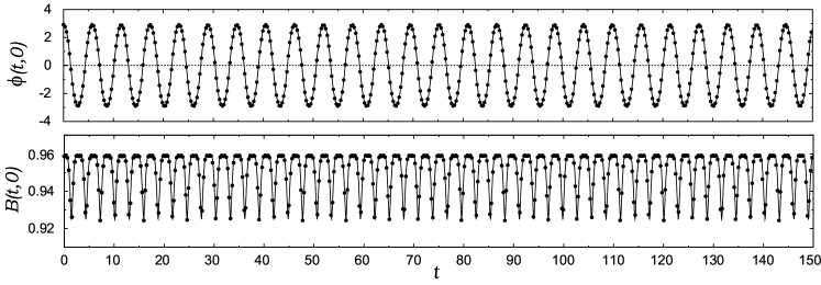
Figure 4: Oscillations of the scalar field (top panel) and metric coefficient (bottom panel) at the center of the pulson for $\varkappa=0.005,\\ a_{max}=0.64$.

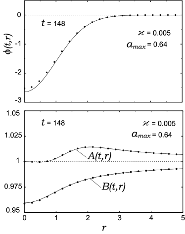
Figure 5: Profiles of the scalar field and metric coefficients.

We have performed the Fourier analysis of the scalar field oscillations obtained by numerical integration of the EKG system. The resulting spectrum shown in Fig. 6(a) demonstrates periodicity with high accuracy.

Then we violated the condition (33) by tripling $X_{1}\left(0\right)$ that was calculated before, and integrated the EKG system again. As expected, the resulting field oscillations were found to be non-periodic. The corresponding spectrum is presented in Fig. 6(b). Nonperiodicity manifests itself as additional peaks in the spectrum which are absent in Fig. 6(a).

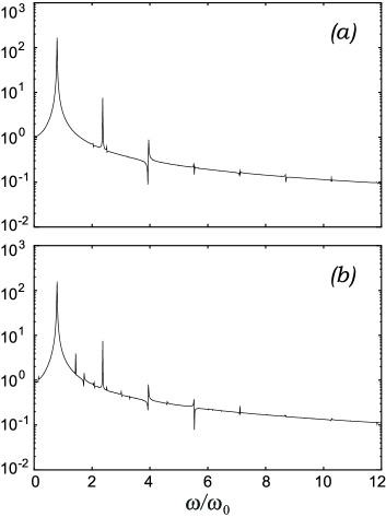
Figure 6: Fourier spectrum of $\phi(t,0)$ for admissible (a) and inadmissible (b) initial conditions.

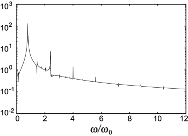
Figure 7: Fourier spectrum of $\phi(t,0)$ obtained from the solution of the nonlinear KG equation (6) with the initial conditions (36), (37). All parameters are the same as in Figs. (4), (5).

To clarify the meaning of gravity, we used the obtained initial conditions (36), (37) with $\varkappa$ as a formal parameter for the numerical integration of the nonlinear KG equation (6). The solution was found to be non-periodic, as is clear from its spectrum which is shown in Fig. 7. We thus conclude that it is because of gravity that the periodic pulsons of the considered non-Gaussian shapes exist.

IV Concluding remarks

Thus we have demonstrated the existence of long-lived time-periodic pulsons in the EKG system. These pulsons differ from the non-gravitating ones in their shapes and frequencies and exist only due to gravitational effects.

The question arises as to whether these gravipulsons are stable. While the stability analysis is out of the scope of the present work, it is worth noting that the stability of the solution (9), and hence (11), is determined by the stability of the solutions of the non-homogeneous Hill’s equation $X_{n}(\theta)$ involved in (16). In turn, as it follows from (24), the stability of the general solution $X_{n}(\theta)$ is determined by the behavior of the functions $X_{n}^{+}(\theta)$ and $X_{n}^{-}(\theta)$.

It is clear that all solutions $X_{n}(\theta)$ satisfying the initial conditions (33), (34) are unstable in the resonance case $\mu_{n}>0$. Indeed, any perturbation of the initial values $X_{n}(0)$, $X_{n\,_{\scriptstyle{\theta}}}(0)$, determined by (33), (34), leads to the appearance of terms $\sim\exp(\mu_{n}\theta)$ on the right-hand side of (24), thus making the corresponding function $X_{n}(\theta)$, and hence the solution (9), exponentially growing in time.

On the other hand, in the non-resonance case $\mu_{n}=i\nu_{n}$, the functions $X_{n}^{+}(\theta)$, $X_{n}^{-}(\theta)$ as well as $X_{n}(\theta)$ in (24) are bounded, and a small perturbation of the initial conditions (33), (34) results in the appearance of only small oscillating terms in $X_{n}(\theta)$. So we can expect that the solution (9) is stable if all modes $X_{n}(\theta)$ are non-resonant. The question is, does any value of $a_{\max}$ exist such that all modes $E_{n}=4n\ (n>0)$ are stable?

A collection of the peaks $\mu_{n}>0$ with $n=1,2,...,10$, shown in Fig. 2, demonstrates the existence of numerous stability intervals separating the instability ones on the $a_{\max}^{2}$ axis. All modes $n=1,2,...,10$ are stable in the gaps between the peaks, and thus $\mu_{n}=i\nu_{n}$. However, if we take into consideration additional modes with $10<n\leqslant N$, supplementary peaks must be added to this plot. Some of the new peaks will be overlapped by the existing ones, but the rest will fall within the stability intervals and erode them. Nevertheless, narrow stability gaps remain visible on the abscise axis even in the case of large $N$.

While we have no proof that some gaps of stability survive as $N$ goes to infinity, one should take into account that the amplitude of the peaks in Fig. 2 decreases with increasing $n$, and in any case, narrow intervals on the $a_{\max}^{2}$ axis can be found where only high-$n$ modes are unstable. We refer to them as intervals of quasi-stability. Indeed, while the solution (9) with $a_{\max}$ falling in one of these intervals is unstable, this instability evolves very slowly, and the gravipulson still remains a long-lived object. Moreover, as it was demonstrated in our simulation Koutvitsky and Maslov (2005), in the case of the non-gravitating pulson, the nonlinear stage of instability saturates very quickly, resulting in a slightly modified pulson which remains a compact oscillating object. We expect the same instability behavior in the case of gravipulsons also, at least at small $\varkappa$, even if this instability is caused by the action of some other perturbative objects around them.

A few words about possible astrophysical applications of the obtained solution are in order. There are a number of papers where scalar solitons are considered as models of galactic halos in hopes of explaining the observational flatness of the rotation curves (see., e.g., Mielke et al. (2005) and references therein). It is easy to see that then the energy density of a scalar field must not decay faster than $r^{-2}$. Evidently, our solution does not satisfy this criterion. However, if a galactic halo is not a single soliton-like object, but is an ensemble of dark matter lumps, of so-called ”mini-MACHOs” Hernández et al. (2004), the gravipulsons may be reasonable candidates for these compact constituents. In this case the gravipulson masses (35) need to be limited by the condition $M\lesssim 10^{-7}M_{\odot}$ following from microlensing data Alcock et al. (1998). This constrains the amplitude of the gravipulsons and the parameters of the potential (2).