$\rho$ Meson Decay in $2+1$ Flavor Lattice QCD

Abstract

We perform a lattice QCD study of the $\rho$ meson decay from the $N_{f}=2+1$ full QCD configurations generated with a renormalization group improved gauge action and a non-perturbatively $O(a)$-improved Wilson fermion action. The resonance parameters, the effective $\rho\to\pi\pi$ coupling constant and the resonance mass, are estimated from the $P$-wave scattering phase shift for the isospin $I=1$ two-pion system. The finite size formulas are employed to calculate the phase shift from the energy on the lattice. Our calculations are carried out at two quark masses, $m_{\pi}=410\,{\rm MeV}$ ($m_{\pi}/m_{\rho}=0.46$) and $m_{\pi}=300\,{\rm MeV}$ ($m_{\pi}/m_{\rho}=0.35$), on a $32^{3}\times 64$ ($La=2.9\,{\rm fm}$) lattice at the lattice spacing $a=0.091\,{\rm fm}$. We compare our results at these two quark masses with those given in the previous works using $N_{f}=2$ full QCD configurations and the experiment.

I Introduction

Recent progress of simulation algorithms, supported by the development of computer power, has made it possible to study hadron physics at the physical quark mass by lattice QCD (see Ref. Rev:DSMI for recent reviews), and lattice calculations have clarified the properties of many hadrons. The studies are mostly concentrated on stable hadrons, however. Resonances pose an important issue both in terms of methodologies and physical results.

Among the resonances, the $\rho$ meson is an ideal case for the lattice calculations, because the final state of the decay is the two-pion state which can be treated on the lattice precisely. In the early stage of studies of the $\rho$ meson decay, the transition amplitude $\langle\pi\pi|\rho\rangle$ extracted from the time behavior of the correlation function $\langle\pi(t)\pi(t)\rho(0)\rangle$ was used to estimate the decay width, assuming that the hadron interaction is small enough so that $\langle\pi\pi|\rho\rangle\ll|\langle\rho|\rho\rangle\langle\pi\pi|\pi\pi\rangle|^{1/2}$ is satisfied rhd:TAMP:GMTW ; rhd:TAMP:LD ; rhd:TAMP:MM ; rhd:TAMP:JMMU .

A more realistic approach is a study from the $P$-wave scattering phase shift for the isospin $I=1$ two-pion system. The finite size formulas presented by Lüscher in the center of mass frame Lfm:L and extensions to non-zero total momentum frames Lfm:RG ; Lfm:ETMC are employed for an estimation of the phase shift from an eigenvalue of the energy on the lattice. The first study of this approach was carried out by CP-PACS Collaboration using $N_{f}=2$ full QCD configurations ($m_{\pi}=330\,{\rm MeV}$, $a=0.21\,{\rm fm}$, $La=2.5\,{\rm fm}$) rhd:SCPH:CP-PACS . After this work ETMC Collaboration presented results with $N_{f}=2$ configurations at several quark masses ($m_{\pi}=290,330\,{\rm MeV}$ ($La=2.5\,{\rm fm}$), $m_{\pi}=420,480\,{\rm MeV}$ ($La=1.9\,{\rm fm}$), $a=0.079\,{\rm fm}$) rhd:SCPH:ETMC_1 ; rhd:SCPH:ETMC_2 . Recently Lang et al. reported results of high statistical calculations with the Laplacian Heaviside smearing operators on a single $N_{f}=2$ gauge ensemble ($m_{\pi}=266\,{\rm MeV}$, $a=0.124\,{\rm fm}$, $La=1.98\,{\rm fm}$) rhd:SCPH:LANG .

In the present work we extend these studies by employing $N_{f}=2+1$ full QCD configurations and working on a larger lattice volume. Our calculations are carried out with the gauge configurations previously generated by PACS-CS Collaboration with a renormalization group improved gauge action and a non-perturbatively $O(a)$-improved Wilson fermion action at $\beta=1.9$ on $32^{3}\times 64$ lattice ($a=0.091\,{\rm fm}$, $La=2.9\,{\rm fm}$) conf:PACS-CS . We choose two subsets of the PACS-CS configurations. One of them corresponds to the hopping parameters $\kappa_{ud}=0.13754$ for the degenerate up and down quarks and $\kappa_{s}=0.13640$ for the strange quark, for which the pion mass takes $m_{\pi}=410\,{\rm MeV}$ ($m_{\pi}/m_{\rho}=0.46$). The other is at $\kappa_{ud}=0.13770$ and $\kappa_{s}=0.13640$, corresponding to $m_{\pi}=300\,{\rm MeV}$ ($m_{\pi}/m_{\rho}=0.35$). We extract the scattering phase shift on three momentum frames, the center of mass and the non-zero momentum frames with the total momentum ${\bf P}=(2\pi/L)(0,0,1)$ and ${\bf P}=(2\pi/L)(1,1,0)$, to obtain the phase shifts at various energies from a single full QCD ensemble as in the previous works by ETMC rhd:SCPH:ETMC_1 ; rhd:SCPH:ETMC_2 and Lang et al. rhd:SCPH:LANG .

We note that QCDSF Collaboration calculated the scattering phase shifts for the ground state in the center of mass frame at several quark masses. ($m_{\pi}=240-430\,{\rm MeV}$) rhd:SCPH:QCDSF . They estimated the resonance parameters from these results, assuming that the effective $\rho\to\pi\pi$ coupling constant does not depend on the quark mass. BMW Collaboration presented their first preliminary results with $N_{f}=2+1$ configurations ($m_{\pi}=200,340\,{\rm MeV}$, $a=0.116\,{\rm fm}$) at Lattice 2010 rhd:SCPH:BMW . We also refer to works exploring an application of the stochastic Laplacian Heaviside smearing to the two-pion states with the isospin $I=0,1,2$ using $N_{f}=2+1$ configurations on the large lattice volume in Ref. rhd:try:HSC .

This paper is organized as follows. In Sec. II we give the method of the calculation. The simulation parameters of the present work are also presented. We present our results and compare ours with those by the other works in Sec. III. Conclusions of the present work are given in Sec. IV. Result of a pilot study of the present work at $m_{\pi}=410\,{\rm MeV}$ was reported at Lattice 2010 rhd:SCPH:PACS-CS . All calculations are carried out on the PACS-CS computer at Center for Computational Sciences, University of Tsukuba.

II Methods

II.1 Finite size formula

In order to calculate the $P$-wave scattering phase shift for the isospin $I=1$ two-pion system at various energies from a single full QCD ensemble, we consider three momentum frames, the center of mass frame (CMF), the non-zero momentum frames with total momentum ${\bf P}=(2\pi/L)(0,0,1)$ (MF1) and ${\bf P}=(2\pi/L)(1,1,0)$ (MF2). These frames have been also considered in the previous works by ETMC rhd:SCPH:ETMC_1 ; rhd:SCPH:ETMC_2 and Lang et al. rhd:SCPH:LANG . In these momentum frames the $P$-wave state is decomposed as

$$\begin{array}[]{lc cc lc lc }\mbox{frame}&&{\bf P}L/(2\pi)&&{\rm g}&&\Gamma\\ \mbox{CMF}&&(0,0,0)&&O_{h}&&{\bf T}_{1}^{-}\\ \mbox{MF1}&&(0,0,1)&&D_{4h}&&{\bf A}_{2}^{-}+{\bf E}^{-}\\ \mbox{MF2}&&(1,1,0)&&D_{2h}&&{\bf B}_{1}^{-}+{\bf B}_{2}^{-}+{\bf B}_{3}^{-}\\ \end{array}\ \ ,$$ (1)

where ${\bf P}$ is the total momentum, ${\rm g}$ is the rotational group in each momentum frame on the lattice and $\Gamma$ is the irreducible representation of the rotational group. In the present work we consider four irreducible representations : ${\bf T}_{1}^{-}$ in the CMF, ${\bf A}_{2}^{-}$ and ${\bf E}^{-}$ in the MF1, and ${\bf B}_{1}^{-}$ in the MF2. The ground and the first excited states of these representations with the isospin $(I,I_{z})=(1,0)$, ignoring the hadron interactions, are shown in Table 1.

The scattering phase shift is related to an eigenvalue of the energy on the lattice by the finite size formula. The formula in the CMF was presented by Lüscher Lfm:L , that in the MF1 by Rummukainen and Gottlieb Lfm:RG , and the MF2 by ETMC Lfm:ETMC . The formulas for the representations considered in the present work are written by

$$\frac{1}{\tan\delta(k)}=\left\{\begin{array}[]{l l }V_{00}&\quad\mbox{ for \,${\bf T}_{1}^{-}$\, in CMF }\\ V_{00}-V_{20}&\quad\mbox{ for \,${\bf E}^{-}$\, in MF1 }\\ V_{00}+2\,V_{20}&\quad\mbox{ for \,${\bf A}_{2}^{-}$\, in MF1 }\\ V_{00}-V_{20}+\sqrt{6}\,V_{22}&\quad\mbox{ for \,${\bf B}_{1}^{-}$\, in MF2 }\end{array}\right.\ ,$$ (2)

with the $P$-wave scattering phase shift $\delta(k)$. The real function $V_{lm}$ is defined by

$$V_{lm}(k;{\bf P})=\frac{1}{\gamma q^{l+1}}\frac{1}{\pi^{3/2}\sqrt{2l+1}}\,e^{-im\pi/4}\cdot Z_{lm}(1;q;{\bf d})\ ,$$ (3)

with ${\bf d}={\bf P}L/(2\pi)$ and $q=kL/(2\pi)$, where ${\bf P}$ is the total momentum and $k$ is the two-pion scattering momentum defined from the invariant mass $\sqrt{s}$ by $\sqrt{s}=\sqrt{E^{2}-|{\bf P}|^{2}}=2\sqrt{k^{2}+m_{\pi}^{2}}$ with the energy $E$ in the non-zero momentum frame. In (3) $\gamma$ is the Lorentz boost factor from the non-zero momentum frame to the center of mass frame given by $\gamma=E/\sqrt{s}$. The function $Z_{lm}(1;q;{\bf d})$ in (3) is an analytic continuation of

$$Z_{lm}(s;q;{\bf d})=\sum_{{\bf r}\in{D({\bf d})}}\,{\cal Y}_{lm}({\bf r})\cdot(|{\bf r}|^{2}-q^{2})^{-s}\ ,$$ (4)

which is defined for ${\rm Re}(s)>(l+3)/2$, where ${\cal Y}_{lm}({\bf r})$ is a polynomial related to the spherical harmonics through ${\cal Y}_{lm}({\bf r})=|{\bf r}|^{l}\cdot Y_{lm}(\Omega)$ with $\Omega$ the spherical coordinate for ${\bf r}$. The convention of $Y_{lm}(\Omega)$ is that of book:MESSIAH . The summation for ${\bf r}$ in (4) runs over the set,

$$D({\bf d})=\left\{\,{\bf r}\,|\,{\bf r}=\hat{\gamma}^{-1}({\bf n}+{\bf d}/2)\,,\,\,{\bf n}\in\mathbb{Z}^{3}\,\right\}\ .$$ (5)

The operation $\hat{\gamma}^{-1}$ is the inverse Lorentz transformation : $\hat{\gamma}^{-1}{\bf x}={\bf x}_{||}/\gamma+{\bf x}_{\bot}$ , where ${\bf x}_{||}=({\bf x}\cdot{\bf d}){\bf d}/{\bf d}^{2}$ is the parallel component and ${\bf x}_{\bot}={\bf x}-{\bf x}_{||}$ is the perpendicular component of the vector ${\bf x}$ in the direction ${\bf d}$. $Z_{lm}(1;q;{\bf d})$ can be evaluated by the method described in Ref. I2_phsh:Yamazaki .

II.2 Extraction of energies

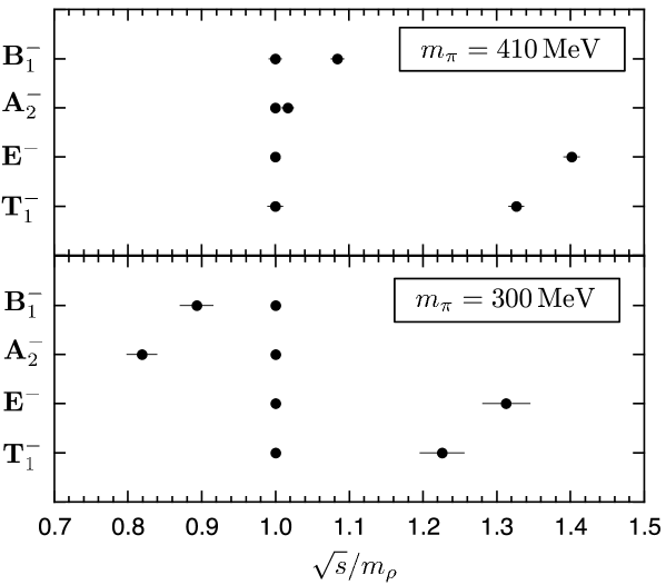
Figure 1: $\sqrt{s}/m_{\rho}$ for states tabulated in Table 1 on our gauge configurations at $m_{\pi}=410\,{\rm MeV}$ (upper panel) and $m_{\pi}=300\,{\rm MeV}$ (lower panel).

In Fig. 1 we show values of the invariant mass $\sqrt{s}$ divided by the $\rho$ meson mass $m_{\rho}$ for the states tabulated in Table 1 on our gauge configurations at $m_{\pi}=410\,{\rm MeV}$ (upper panel) and $m_{\pi}=300\,{\rm MeV}$ (lower panel). Here we ignore the hadron interactions and use the values of $m_{\rho}$ and $m_{\pi}$ obtained in the previous work in Ref. conf:PACS-CS . For the ${\bf T}^{-}_{1}$ and the ${\bf E}^{-}$ representation, we only calculate the scattering phase for the ground state in the present work. From Fig. 1 the energies of these states are expected to be much smaller than those of the excited states, even if the hadron interaction is switched on. Thus, we extract the energies of these states by a single exponential fit for the time correlation functions of the $\rho$ meson as carried out in a usual study of the hadron spectrum. We use the local $\rho$ meson operator for the sink and a smeared operator for the source as discussed later.

For the ${\bf A}_{2}^{-}$ and the ${\bf B}_{1}^{-}$ representation, we also calculate the scattering phase shift for the first excited state. In order to extract the energies of the lower two states for these representations, we use the variational method method_diag:LW with a matrix of the time correlation function,

$$G(t)=\left(\begin{array}[]{ll}\langle 0|\,(\pi\pi)^{\dagger}(t)\,\overline{(\pi\pi)}(t_{s})\,|0\rangle&\,\,\langle 0|\,(\pi\pi)^{\dagger}(t)\,\overline{\rho}(t_{s})\,|0\rangle\\ \langle 0|\,\rho^{\dagger}(t)\,\overline{(\pi\pi)}(t_{s})\,|0\rangle&\,\,\langle 0|\,\rho^{\dagger}(t)\,\overline{\rho}(t_{s})\,|0\rangle\end{array}\right)\ ,$$ (6)

for each representation. The energies are extracted from two eigenvalues $\lambda_{n}(t)$ ($n=1,2$) of the matrix,

$$M(t)=G(t)\,G^{-1}(t_{R})\ ,$$ (7)

with some reference time $t_{R}$.

Here we comment on the discussion of the generalized eigenvalue problem (GEVP) by ALPHA Collaboration in Ref. method_GEVP . In a $2\times 2$ matrix case of $G(t)$, they proved that the effective mass of the eigenvalue $\lambda_{n}(t)$ ($n=1,2$) of the matrix $M(t)$ in (7) can be written as

$$E_{n}+O({\rm e}^{-(E_{m}-E_{n})t})\qquad(n=1,2\ ,\ m\geq 3)\ ,$$ (8)

in a large time region with the eigenvalue of the energy $E_{i}$ ($i=1,2,\cdots$ ). Here it should be noted that their proof was given only for the case where $G(t)$ is a Hermitian matrix. In our case we use different operators for the sink and source in $G(t)$ as explained later. Therefore $G(t)$ is not a Hermitian matrix and the discussion of GEVP cannot be applied to our case. In the present work we assume that the lower two states dominate $G(t)$ in a large time region. This is expected to be a good approximation, because the second excited state takes a much higher value ( $E_{3}/E_{2}>1.3$ in the absence of hadron interactions for both quark masses studied in the present work ). With this assumption, the second term of (8) does not appear for a general case of $G(t)$, and the energy for the ground and the first excited states can be extracted by a single exponential fit for the eigenvalue $\lambda_{n}(t)$ ($n=1,2$) in a large $t$ region.

In (6) the operator $\rho(t)$ is given by

$$\rho(t)=\sum_{j=1}^{3}\,p_{j}\cdot\rho_{j}({\bf p},t)/|{\bf p}|\ ,$$ (9)

where $\rho_{j}({\bf p},t)$ is the local operator for the neutral $\rho$ meson at the time slice $t$ with the momentum ${\bf p}$. The momentum takes ${\bf p}=(2\pi/L)(0,0,1)$ for the ${\bf A}_{2}^{-}$ and ${\bf p}=(2\pi/L)(1,1,0)$ for the ${\bf B}_{1}^{-}$ representation. Hereafter we assume that the momentum ${\bf p}$ takes one of these two values depending on the representation.

In (6) $(\pi\pi)(t)$ is an operator for the two pions with the momentum ${\bf 0}$ and ${\bf p}$, which is defined by

$$(\pi\pi)(t)=\frac{1}{\sqrt{2}}\left(\pi^{+}({\bf 0},t_{1})\,\pi^{-}({\bf p},t)-\pi^{-}({\bf 0},t_{1})\,\pi^{+}({\bf p},t)\right)\times{\rm e}^{m_{\pi}\cdot(t_{1}-t)}\ ,$$ (10)

where $\pi^{\pm}({\bf p},t)$ is the local pion operator with the momentum ${\bf p}$ at the time slice $t$. The time slice of the pion with the zero momentum is fixed at $t_{1}\gg t$, and the time slice of the other pion $t$ runs over the whole time extent. An exponential time factor in (10) is introduced so that the operator has the same time behavior as that of the usual Heisenberg operator, i.e.,

$$\langle 0|\,(\pi\pi)^{\dagger}(t)=\langle 0|\,(\pi\pi)^{\dagger}(0)\,{\rm e}^{-Ht}\qquad\mbox{ for $t_{1}\gg t$ }\ ,$$ (11)

with the Hamiltonian $H$.

In the previous works the time slices of the two operators for the pion in the sink operator (10) are set equal $t_{1}=t$, and they simultaneously run over some time interval. In that case we need to repeat solving quark propagators for the time slices in that time interval. This computer-time consuming procedure can be avoided by fixing the time slice of one of the pion at $t_{1}$ as done in the present work. But we need to set $t_{1}\gg t$ to avoid contamination from higher energy states produced by the operator at $t_{1}$ in this method.

Two operators $\overline{(\pi\pi)}(t_{s})$ and $\overline{\rho}(t_{s})$ are used for the sources in (6), which are given by

$$\overline{(\pi\pi)}(t_{s})=\frac{1}{\sqrt{2}}\Bigl{(}\pi^{+}({\bf 0},t_{s})\pi^{-}({\bf p},t_{s})-\pi^{-}({\bf 0},t_{s})\pi^{+}({\bf p},t_{s})\Bigl{)}\ ,$$ (12)

$$\overline{\rho}(t_{s})=\frac{1}{N_{\Gamma}}\sum_{{\bf z}\in\Gamma}\frac{1}{\sqrt{2}}\Bigl{(}\overline{U}({\bf z},t_{s})\gamma_{p}U({\bf z},t_{s})-\overline{D}({\bf z},t_{s})\gamma_{p}D({\bf z},t_{s})\Bigl{)}{\rm e}^{i{\bf p}\cdot{\bf z}}\ ,$$ (13)

where $\gamma_{p}=\sum_{j=1}^{3}p_{j}\cdot\gamma_{j}/|{\bf p}|$. The operator $Q({\bf z},t_{s})$ ($Q=U,D$) is a smeared operator for the up or the down quark given by

$$Q({\bf z},t_{s})=\sum_{\bf{}_{x}}q({\bf x},t_{s})\cdot\Psi(|{\bf x}-{\bf z}|)\ ,$$ (14)

where $q({\bf x},t_{s})$ ($q=u,d)$ is the up or the down quark operator at the position ${\bf x}$ and the time $t_{s}$. We adopt the same smearing function $\Psi(|{\bf x}|)$ as in Ref. conf:PACS-CS , i.e., $\Psi(|{\bf x}|)=A\exp(-B|{\bf x}|)$ with $\Psi(0)=1$ and the smearing parameters : $(A,B)=(1.2,0.17)$ for $m_{\pi}=410\,{\rm MeV}$ and $(A,B)=(1.2,0.09)$ for $m_{\pi}=300\,{\rm MeV}$. The operator (14) is used after fixing gauge configurations to the Coulomb gauge, assuming that an ambiguity of the gauge fixing does not cause a significant systematic error in the time correlation function. In (13) a summation over ${\bf z}$ is taken to reduce a statistical error and

$$\Gamma=\{\ {\bf z}\ |\ {\bf z}=(L/2)\cdot(n_{1},n_{2},n_{3})\ ,\ n_{j}=\mbox{$0$ or $1$}\ ,\ N_{\Gamma}=8\ \}$$ (15)

is chosen in the present work. The smeared operator (13) is also used to extract the energy of the ground state for the ${\bf T}_{1}^{-}$ and the ${\bf E}^{-}$ representation, setting the momentum ${\bf p}={\bf 0}$ and ${\bf p}=(2\pi/L)(0,0,1)$, respectively.

Here we note that the operator $(\pi\pi)(t)$ in (10) is not an eigenstate under exchange of the momenta of the two pions. Thus it has no definite parity and does not belong to the irreducible representation of the $D_{4h}$ for ${\bf p}=(2\pi/L)(0,0,1)$ and the $D_{2h}$ for ${\bf p}=(2\pi/L)(1,1,0)$. It is actually a linear combination of components of two irreducible representations ${\bf A}_{2}^{-}+{\bf A}_{1}^{+}$ for the $D_{4h}$ and ${\bf B}_{1}^{-}+{\bf A}_{1}^{+}$ for the $D_{2h}$. The other operators in $G(t)$ in (6), however, belong to the irreducible representation ${\bf A}_{2}^{-}$ or ${\bf B}_{1}^{-}$ depending on the momentum ${\bf p}$. Therefore, it is not necessary to worry about mixing to other irreducible representations in $G(t)$ in (6).

II.3 Calculation of $G(t)$

The quark contractions of the components of the matrix of the time correlation function $G(t)$ in (6) are shown in Fig. 2. The time runs upward in the diagrams. The vertices refer to the pion or the $\rho$ meson operator with the momentum at the time slice specified in the diagrams. The momentum ${\bf p}$ takes ${\bf p}=(2\pi/L)(0,0,1)$ for the ${\bf A}_{2}^{-}$ and ${\bf p}=(2\pi/L)(1,1,0)$ for the ${\bf B}_{1}^{-}$ representation. The $\rho$ meson operators at $t_{s}$ are the smeared operators and the other is the local operator.

We calculate the quark contractions in Fig. 2 by the source method and the stochastic noise method as in the previous work by CP-PACS rhd:SCPH:CP-PACS . We introduce a $U(1)$ noise $\xi_{j}({\bf x})$ which satisfies

$$\sum_{j=1}^{N_{R}}\xi_{j}^{\dagger}({\bf x})\xi_{j}({\bf y})=\delta^{3}({\bf x}-{\bf y})\qquad\mbox{ for \ $N_{R}\to\infty$ }\ ,$$ (16)

where $N_{R}$ is the number of noises. We calculate the following four types of quark propagators:

$$Q_{AB}({\bf x},t|{\bf q},t_{s},\xi_{j})=\sum_{\bf y}(D^{-1})_{AB}({\bf x},t;{\bf y},t_{s})\cdot\Bigl{[}{\rm e}^{i{\bf q}\cdot{\bf y}}\xi_{j}({\bf y})\Bigr{]}\ ,$$ (17)

$$W_{AB}({\bf x},t|{\bf k},t_{a}|{\bf q},t_{s},\xi_{j})=\sum_{\bf y}\sum_{C}(D^{-1})_{AC}({\bf x},t;{\bf y},t_{a})\cdot\Bigl{[}{\rm e}^{i{\bf k}\cdot{\bf y}}\gamma_{5}\ Q({\bf y},t_{a}|{\bf q},t_{s},\xi_{j})\Bigr{]}_{CB}\ ,$$ (18)

$$\overline{Q}_{AB}({\bf x},t|{\bf z},t_{s})=\sum_{\bf y}(D^{-1})_{AB}({\bf x},t;{\bf y},t_{s})\cdot\Bigl{[}\Psi(|{\bf y}-{\bf z}|)\Bigr{]}\ ,$$ (19)

$$\overline{W}_{AB}({\bf x},t|{\bf k},t_{a}|{\bf z},t_{s})=\sum_{\bf y}\sum_{C}(D^{-1})_{AC}({\bf x},t;{\bf y},t_{a})\cdot\Bigl{[}{\rm e}^{i{\bf k}\cdot{\bf y}}\gamma_{5}\ \overline{Q}({\bf y},t_{a}|{\bf z},t_{s})\Bigr{]}_{CB}\ ,$$ (20)

where $A$, $B$ and $C$ refer to color and spin indices, and $\Psi(|{\bf x}|)$ is the smearing function in (14). The square bracket is used as the source for the inversion of the Dirac operator $D$. The propagators for the smeared quarks ($\overline{Q}$ and $\overline{W}$) are solved on the gauge configurations fixed to the Coulomb gauge, while the gauge is not fixed for those of the stochastic quarks ($Q$ and $W$).

The function $G_{\pi\pi\to\pi\pi}(t)$ for the first diagram in Fig. 2 can be calculated by introducing an another $U(1)$ noise $\eta_{j}({\bf x})$ having the same property as $\xi_{j}({\bf x})$ in (16),

$$G^{\rm[1st]}_{\pi\pi\to\pi\pi}(t) = \sum_{j=1}^{N_{R}}\sum_{{\bf x},{\bf y}}\Bigl{\langle}Q^{\dagger}({\bf x},t_{1}|{\bf 0},t_{s},\eta_{j})\,Q({\bf x},t_{1}|{\bf 0},t_{s},\eta_{j})\Bigr{\rangle}\,{\rm e}^{m_{\pi}\cdot(t_{1}-t)}$$ (22)

$$\quad\times\,\,{\rm e}^{-i{\bf p}\cdot{\bf y}}\Bigl{\langle}Q^{\dagger}({\bf y},t|{\bf 0},t_{s},\xi_{j})\,Q({\bf y},t|{\bf p},t_{s},\xi_{j})\Bigr{\rangle}\ ,$$

where the bracket means trace for the color and the spin indices. The exponential time factor comes from the definition of the operator for the two pions in (10). The $G_{\pi\pi\to\pi\pi}(t)$ for the second diagram is given by exchanging the momentum and the time slice of the sink in (22).

The function $G_{\pi\pi\to\pi\pi}(t)$ for the 3rd to 6th diagrams can be obtained by

$$G^{\rm[3rd]}_{\pi\pi\to\pi\pi}(t) = \sum_{j=1}^{N_{R}}\sum_{\bf x}{\rm e}^{-i{\bf p}\cdot{\bf x}}\Bigl{\langle}W^{\dagger}({\bf x},t|{\bf 0},t_{1}|{\bf 0},t_{s},\xi_{j})\,W({\bf x},t|{\bf 0},t_{s}|{\bf p},t_{s},\xi_{j})\Bigr{\rangle}{\rm e}^{m_{\pi}\cdot(t_{1}-t)}\ ,$$ (23)

$$G^{\rm[4th]}_{\pi\pi\to\pi\pi}(t) = \sum_{j=1}^{N_{R}}\sum_{\bf x}{\rm e}^{-i{\bf p}\cdot{\bf x}}\Bigl{\langle}W^{\dagger}({\bf x},t|{\bf 0},t_{1}|{\bf 0},t_{s},\xi_{j})\,W({\bf x},t|{\bf p},t_{s}|{\bf 0},t_{s},\xi_{j})\Bigr{\rangle}{\rm e}^{m_{\pi}\cdot(t_{1}-t)}\ ,$$ (24)

$$G^{\rm[5th]}_{\pi\pi\to\pi\pi}(t) = \sum_{j=1}^{N_{R}}\sum_{\bf x}{\rm e}^{-i{\bf p}\cdot{\bf x}}\Bigl{\langle}W({\bf x},t|{\bf 0},t_{1}|{\bf 0},t_{s},\xi_{j})\,W^{\dagger}({\bf x},t|{\bf 0},t_{s}|-{\bf p},t_{s},\xi_{j})\Bigr{\rangle}{\rm e}^{m_{\pi}\cdot(t_{1}-t)}\ ,$$ (25)

$$G^{\rm[6th]}_{\pi\pi\to\pi\pi}(t) = \sum_{j=1}^{N_{R}}\sum_{\bf x}{\rm e}^{-i{\bf p}\cdot{\bf x}}\Bigl{\langle}W({\bf x},t|{\bf 0},t_{1}|{\bf 0},t_{s},\xi_{j})\,W^{\dagger}({\bf x},t|-{\bf p},t_{s}|{\bf 0},t_{s},\xi_{j})\Bigr{\rangle}{\rm e}^{m_{\pi}\cdot(t_{1}-t)}\ .$$ (26)

The function $G_{\pi\pi\to\rho}(t)$ for two diagrams in Fig. 2 can be similarly calculated by

$$G^{\rm[1st]}_{\pi\pi\to\rho}(t) = \sum_{j=1}^{N_{R}}\sum_{\bf x}{\rm e}^{-i{\bf p}\cdot{\bf x}}\Bigl{\langle}W^{\dagger}({\bf x},t|-{\bf p},t_{s}|{\bf 0},t_{s},\xi_{j})\,(\gamma_{5}\gamma_{p})\,Q({\bf x},t|{\bf 0},t_{s},\xi_{j})\Bigr{\rangle}\ ,$$ (27)

$$G^{\rm[2nd]}_{\pi\pi\to\rho}(t) = \sum_{j=1}^{N_{R}}\sum_{\bf x}{\rm e}^{-i{\bf p}\cdot{\bf x}}\Bigl{\langle}Q^{\dagger}({\bf x},t|{\bf 0},t_{s},\xi_{j})\,(\gamma_{5}\gamma_{p})\,W({\bf x},t|{\bf p},t_{s}|{\bf 0},t_{s},\xi_{j})\Bigr{\rangle}\ ,$$ (28)

where $\gamma_{p}=\sum_{j=1}^{3}p_{j}\cdot\gamma_{j}/|{\bf p}|$.

We can obtain the function $G_{\rho\to\pi\pi}(t)$ for two diagrams in Fig. 2 by

$$G^{\rm[1st]}_{\rho\to\pi\pi}(t) = -\frac{1}{N_{\Gamma}}\sum_{{\bf z}\in\Gamma}{\rm e}^{i{\bf p}\cdot{\bf z}}\sum_{\bf x}{\rm e}^{-i{\bf p}\cdot{\bf x}}\Bigl{\langle}\overline{Q}^{\dagger}({\bf x},t|{\bf z},t_{s})\,\overline{W}({\bf x},t|{\bf 0},t_{1}|{\bf z},t_{s})\,(\gamma_{5}\gamma_{p})\Bigr{\rangle}{\rm e}^{m_{\pi}\cdot(t_{1}-t)}\ ,$$ (29)

$$G^{\rm[2nd]}_{\rho\to\pi\pi}(t) = -\frac{1}{N_{\Gamma}}\sum_{{\bf z}\in\Gamma}{\rm e}^{i{\bf p}\cdot{\bf z}}\sum_{\bf x}{\rm e}^{-i{\bf p}\cdot{\bf x}}\Bigl{\langle}\overline{W}^{\dagger}({\bf x},t|{\bf 0},t_{1}|{\bf z},t_{s})\,\overline{Q}({\bf x},t|{\bf z},t_{s})\,(\gamma_{5}\gamma_{p})\Bigr{\rangle}{\rm e}^{m_{\pi}\cdot(t_{1}-t)}\ ,$$ (30)

where $\Gamma$ and $N_{\Gamma}$ are defined by (15). The component $G_{\rho\to\rho}(t)$ is given by the $\overline{Q}$-type propagators as the usual time correlation function for the $\rho$ meson,

$$G_{\rho\to\rho}(t)=-\frac{1}{N_{\Gamma}}\sum_{{\bf z}\in\Gamma}{\rm e}^{i{\bf p}\cdot{\bf z}}\sum_{\bf x}{\rm e}^{-i{\bf p}\cdot{\bf x}}\Bigl{\langle}\overline{Q}^{\dagger}({\bf x},t|{\bf z},t_{s})(\gamma_{5}\gamma_{p})\,\overline{Q}({\bf x},t|{\bf z},t_{s})\,(\gamma_{5}\gamma_{p})\Bigr{\rangle}\ .$$ (31)

We calculate the $Q$-type propagators (17) for combinations of ${\bf q}$ and $U(1)$ noise :

$$({\bf q},{\rm noise})=\{\,({\bf 0},\xi),({\bf 0},\eta),({\bf p},\xi),(-{\bf p},\xi)\,\}\ ,$$ (32)

and $W$-type propagators (18) for combinations of ${\bf k}$, $t_{a}$ and ${\bf q}$ :

$$({\bf k},t_{a}|{\bf q})=\{\,({\bf p},t_{S}|{\bf 0}),(-{\bf p},t_{S}|{\bf 0}),({\bf 0},t_{S}|{\bf p}),({\bf 0},t_{S}|-{\bf p}),({\bf 0},t_{1}|{\bf 0})\,\}\ ,$$ (33)

using the same $U(1)$ noise $\xi$ in common. The $\overline{Q}$-type (19) and the $\overline{W}$-type propagator (20) for $({\bf k},t_{a})=({\bf 0},t_{1})$ are solved for the set ${\bf z}\in{\Gamma}$.

II.4 Simulation parameters

Calculations in the present work employ $N_{f}=2+1$ full QCD configurations previously generated by PACS-CS using a renormalization group improved gauge action and a non-perturbatively $O(a)$-improved Wilson fermion action at $\beta=1.9$ on $32^{3}\times 64$ lattice ($a=0.091\,{\rm fm}$, $La=2.9\,{\rm fm}$) conf:PACS-CS . We choose two subsets of the PACS-CS configurations. One of them corresponds to the hopping parameters $\kappa_{ud}=0.13754$ for the degenerate up and down quarks and $\kappa_{s}=0.13640$ for the strange quark, for which the pion mass takes $m_{\pi}=410\,{\rm MeV}$ ($m_{\pi}/m_{\rho}=0.46$). The total number of configurations analyzed every $10$ trajectories is $440$. We estimate the statistical errors by the jackknife method with bins of $400$ trajectories. The other set is at $\kappa_{ud}=0.13770$ and $\kappa_{s}=0.13640$, corresponding to $m_{\pi}=300\,{\rm MeV}$ ($m_{\pi}/m_{\rho}=0.35$). The total number of configurations of this set is $400$ and the measurements are done every $20$ trajectories. The statistical errors are estimated by the jackknife method with bins of $800$ trajectories.

The periodic boundary conditions are imposed for both spatial and temporal directions in configuration generations. We impose the Dirichlet boundary condition for the temporal direction at $t=0$ and $t=T$ in calculations of the quark propagators, to avoid the unwanted thermal contributions produced by propagating two pions in opposite directions in a time. For both quark masses, we set the source operators $\overline{(\pi\pi)}(t_{s})$ in (12) and $\overline{\rho}(t_{s})$ in (13) at $t_{s}=12$ to avoid effects from the temporal boundary, and the zero momentum pion in the sink operator $(\pi\pi)(t)$ in (10) at $t_{1}=42$.

In order to see effects from the Dirichlet boundary, we calculate the time correlation functions of the single meson channels setting the source at $t_{s}=12$ with the Dirichlet boundary condition. We compare these with those obtained with the periodic boundary condition in the previous work in Ref. conf:PACS-CS , and find no difference beyond statistical fluctuations between them. This shows that $t_{s}=12$ is sufficiently large to avoid effects from the boundary for the single meson channels. We assume from this that $t_{s}=12$ and $t_{1}=42$ ($22$ away from the boundary) are safe distances to avoid effects from the boundary also for the time correlation functions of the two-pion state. We find that the effective mass of the time correlation function for the pion with the zero momentum reaches plateau after $t-t_{s}=12$ for the both quark masses. We can expect from this that the eigenvalues $\lambda_{n}(t)$ ($n=1,2$) of the matrix $M(t)$ in (7) have a single exponential behaviors in a time range $t\leq t_{1}-12$ ($=30$).

In a pilot study of the present work at $m_{\pi}=410\,{\rm MeV}$, calculations of the phase shift were carried out only for three representations, ${\bf T}_{1}^{-}$, ${\bf E}^{-}$ and ${\bf A}_{2}^{-}$, setting the number of the random noise $N_{R}=10$ in (16). The results on this pilot study have been reported in Ref. rhd:SCPH:PACS-CS . We found from this study that errors from a finiteness of the number of the random noise are small enough compared with the statistical error for three representations even if we take $N_{R}=2$. Assuming that this observation applies also for both quark masses and all representations in the present work, we set $N_{R}=2$ for all calculations after this pilot study.

In order to reduce the statistical error, we carry out additional measurements shifting the time slice of the source operators $t_{s}$, the zero momentum pion in the sink operator $t_{1}$ and the Dirichlet boundary condition by a time shift $\Delta t$ simultaneously, and average over these measurements. For $m_{\pi}=410\,{\rm MeV}$, the measurement of the pilot study for the three representations was done without shifting the time slices. We carry out additional measurements for all representations with the time shift $\Delta t=T/2$ and $T/4$. We average over these two measurements for the ${\bf B}_{1}^{-}$ representation and all three measurements for three representations, ${\bf T}_{1}^{-}$, ${\bf E}^{-}$ and ${\bf A}_{2}^{-}$. For $m_{\pi}=300\,{\rm MeV}$, the measurements for all representations are carried out with the time shift $\Delta t=0$ and $T/2$, and are averaged.

III Results

III.1 Time correlation function

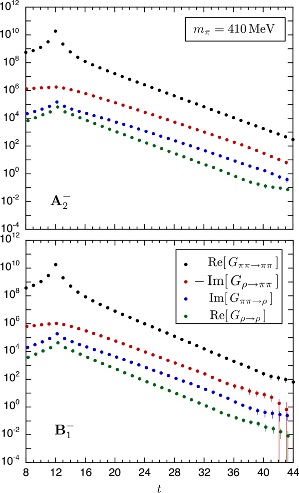
Figure 3: Four components of the matrix of the time correlation function $G(t)$ at $m_{\pi}=410\,{\rm MeV}$ for the ${\bf A}_{2}^{-}$ (upper panel) and for the ${\bf B}_{1}^{-}$ representation (lower panel). Same symbols for the components are used in both panels. The source operators $\overline{(\pi\pi)}(t_{s})$ and $\overline{\rho}(t_{s})$ are located at $t_{s}=12$. The pion with the zero momentum in the sink operator $(\pi\pi)(t)$ in (10) is set at $t_{1}=42$.

In Fig. 3 we show the real part of the diagonal components ($\pi\pi\to\pi\pi$ and $\rho\to\rho$ ) and imaginary part of the off-diagonal components ($\rho\to\pi\pi$ and $\pi\pi\to\rho$) of the matrix of the time correlation function $G(t)$ in (6) for the ${\bf A}_{2}^{-}$ and the ${\bf B}_{1}^{-}$ representation at $m_{\pi}=410\,{\rm MeV}$. We note that the diagonal components are real and the off-diagonal components are pure imaginary by $P$ and $CP$ symmetry. Choosing $t_{R}=23$ as the reference time of the variational method for the matrix $M(t)$ in (7), we obtain the two eigenvalues $\lambda_{1}(t)$ and $\lambda_{2}(t)$ of the matrix, which corresponds to the correlation function for the ground and the first excited state respectively, for each representation.

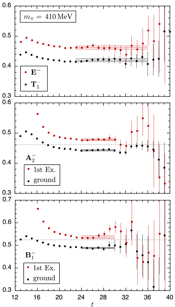
Figure 4: Effective masses of the ground state for the ${\bf T}_{1}^{-}$ and the ${\bf E}^{-}$ representation, and the ground and first excited states for the ${\bf A}_{2}^{-}$ and ${\bf B}_{1}^{-}$ representation at $m_{\pi}=410\,{\rm MeV}$. The source operators $\overline{(\pi\pi)}(t_{s})$ and $\overline{\rho}(t_{s})$ are located at $t_{s}=12$. For the ${\bf A}_{2}^{-}$ and ${\bf B}_{1}^{-}$ representation, we set the pion with the zero momentum in the sink operator $(\pi\pi)(t)$ in (10) at $t_{1}=42$ and the reference time of the variational method at $t_{R}=23$. The results of the fitting with one standard deviation error band are expressed by solid lines. The dotted lines for the the ${\bf A}_{2}^{-}$ and ${\bf B}_{1}^{-}$ representation indicate the energies of the two free pions.

The effective masses of the time correlation functions for six states considered in the present work at $m_{\pi}=410\,{\rm MeV}$ are plotted in Fig. 4. We can find plateaus in the time region $t\geq 23$. The results of the energies $E$ extracted by a single exponential fit for these time correlation functions are tabulated in Table 2, together with adopted fitting ranges. We choose smaller value for the maximum time of the fitting range for the ${\bf A}_{2}^{-}$ and the ${\bf B}_{1}^{-}$ representation than those for the others to avoid contamination from higher energy states produced by the zero momentum pion at $t_{1}=42$ in the sink operator $(\pi\pi)(t)$ in (10). In Fig. 4 the results of the fitting with one standard deviation error band are also expressed by solid lines. The dotted line for the ${\bf A}_{2}^{-}$ and ${\bf B}_{1}^{-}$ representation in the figure indicates the energy of the two free pions for each representation.

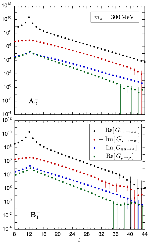
Figure 5: Same as Fig. 3 for $m_{\pi}=300\,{\rm MeV}$.

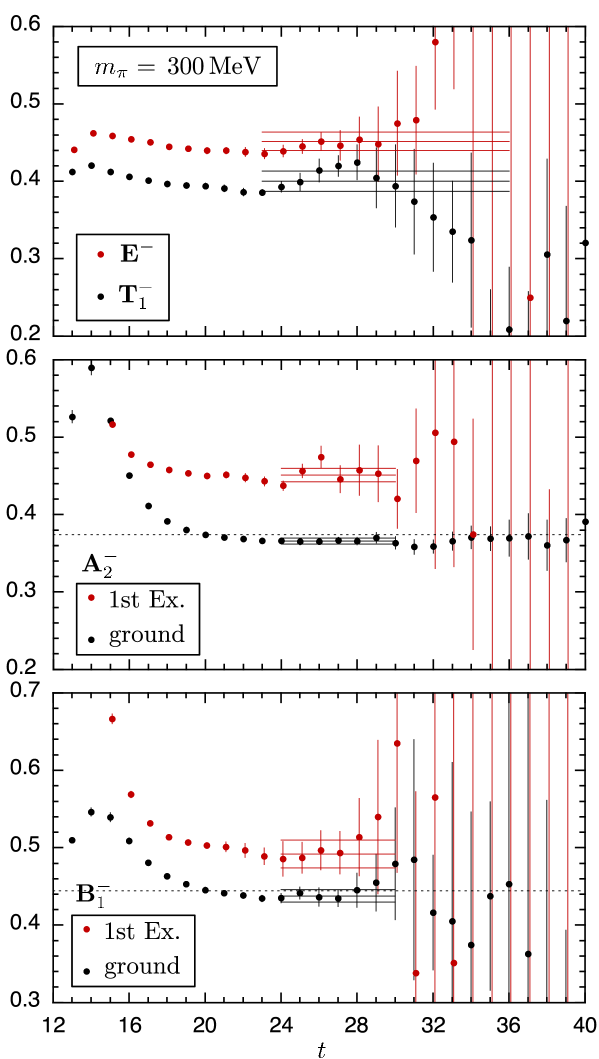
Figure 6: Same as Fig. 4 for $m_{\pi}=300\,{\rm MeV}$.

The components of the matrix of the time correlation function $G(t)$ at $m_{\pi}=300\,{\rm MeV}$ are plotted in Fig. 5 and the effective masses in Fig. 6, where $t_{R}=23$ is also chosen as the reference time. The statistics is less than that at $m_{\pi}=410\,{\rm MeV}$, but we also see plateaus in the effective masses for $t\geq 23$. The results of the energies $E$ extracted by a single exponential fit are tabulated in Table 3.

In the previous work by CP-PACS, carried out at the lattice spacing $a=0.21\,{\rm fm}$, they found a large violation of the continuum dispersion relation for the single pion state due to the discretization error on their gauge configurations. The discretization error also affects calculations of the invariant mass $\sqrt{s}$ and the scattering momentum $k$ for the two-pion system since they are evaluated from the energy $E$. The continuum relation is given by $\sqrt{s}=\sqrt{E^{2}-|{\bf P}|^{2}}=2\sqrt{k^{2}+m_{\pi}^{2}}$, while there are several alternatives on the lattice, e.g.,

$${\rm cosh}(\sqrt{s})={\rm cosh}(E)-2\sum_{j=1}^{3}\sin^{2}(P_{j}/2)\ ,$$ (34)

$$2\cdot\sin^{2}(k/2)={\rm cosh}(\sqrt{s}/2)-{\rm cosh}(m_{\pi})\ .$$ (35)

The two-pion scattering momentum cannot be uniquely defined due to the breaking of the translational and rotational symmetries in the finite lattice spacing as mentioned in Ref. Lfm:RG . The momentum $k$ given by (35) is just one of the choices of the momentum, thus the discretization error cannot be fully avoided by using (34) and (35). In the work by CP-PACS, they regarded the difference of the final results for the choice of the relations as the systematic error from the discretization error.

We also monitor the validity of the continuum dispersion relation for the single pion state and find that the violation is negligible in the present work, one reason being that our lattice spacing $a=0.091\,{\rm fm}$ is much smaller than that for the CP-PACS case. We compare the energy $E$ extracted from the the time correlation function with that given by the dispersion relation $E_{\rm eff}=\sqrt{|{\bf p}|^{2}+m_{\pi}^{2}}$ from the mass $m_{\pi}$ and the momentum ${\bf p}$. The results for $m_{\pi}=410\,{\rm MeV}$ are $E/E_{\rm eff}=0.9988(15)$ for ${\bf p}=(2\pi/L)(0,0,1)$ and $0.9988(63)$ for ${\bf p}=(2\pi/L)(1,1,0)$. Those for $m_{\pi}=300\,{\rm MeV}$ are $0.9924(81)$ and $0.984(16)$. Therefore, the violation of the dispersion relation for the single pion state is not seen on our gauge configurations. We also evaluate $\sqrt{s}$ for the two-pion state by (34), but we see no difference over the statistics from that given by the relation in the continuum. From this we calculate $\sqrt{s}$ and $k$ from $E$ by the relation in the continuum, avoiding ambiguities possibly caused by the choice of the relations. The results given by this way are tabulated in Table 2 and Table 3.

III.2 Scattering phase shift and resonance parameters

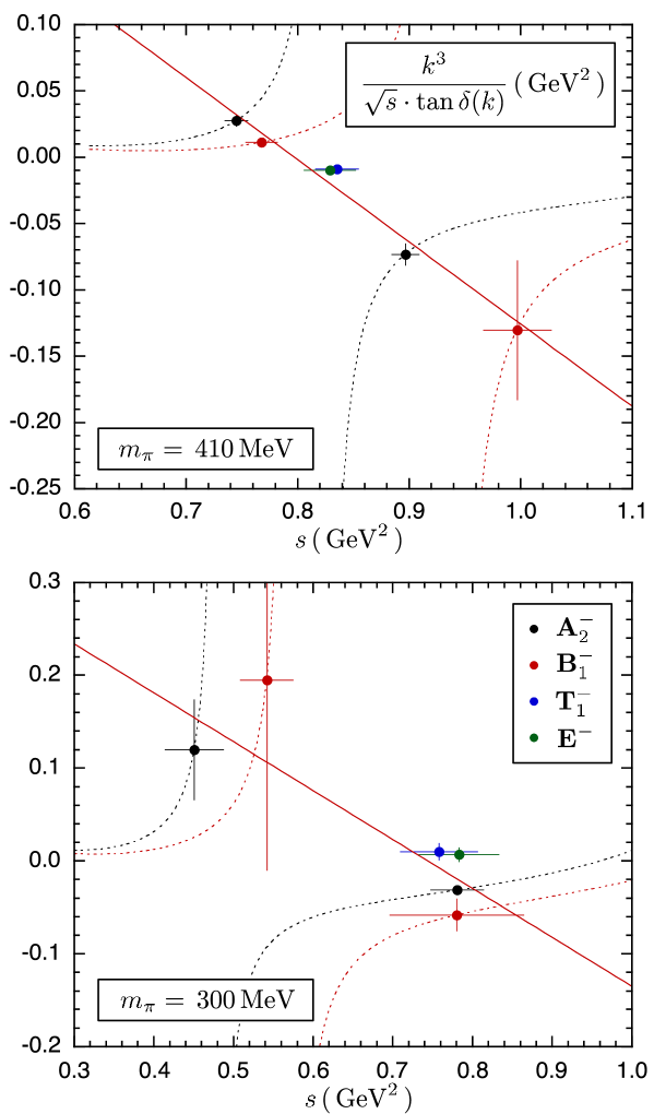
Figure 7: $k^{3}/(\sqrt{s}\cdot\tan\delta(k))$ as a function of square of the invariant mass ${s}$ at $m_{\pi}=410\,{\rm MeV}$ (upper panel) and $m_{\pi}=300\,{\rm MeV}$ (lower panel). Same symbols for four representations are used in both panels. Dotted lines are the finite size formulas for the ${\bf A}_{2}^{-}$ and the ${\bf B}_{1}^{-}$ representation. A solid line for each quark mass is a fitting line by (36).

The scattering phase shift $\delta(k)$ obtained by substituting the scattering momentum $k$ and the total momentum ${\bf P}$ into the finite size formulas in (2) are presented in the lower part of Table 2 for $m_{\pi}=410\,{\rm MeV}$ and Table 3 for $m_{\pi}=300\,{\rm MeV}$. We use the lattice spacing determined from $m_{\Omega}$ in Ref. conf:PACS-CS , $a=0.0907(13)\,{\rm fm}$ ($1/a=2.176(31)\,{\rm GeV}$), to get the values in the physical unit, where the error of the lattice spacing is not included. In Fig. 7 the results of $k^{3}/(\sqrt{s}\cdot\tan\delta(k))$ are plotted as a function of square of the invariant mass $s$ for $m_{\pi}=410\,{\rm MeV}$ (upper panel) and $m_{\pi}=300\,{\rm MeV}$ (lower panel). The finite size formulas for the ${\bf A}_{2}^{-}$ and the ${\bf B}_{1}^{-}$ representation are plotted by dotted lines. Divergent point on these lines corresponds to the square of the invariant mass of the two free pions. In the figure the error bars of $s$ and $k^{3}/(\sqrt{s}\cdot\tan\delta(k))$ are plotted regarding them as independent. But these are fully correlated by the finite size formula, so the true error lies along the dotted line corresponding to the formula. Thus, the error bars in the figure indicate projections of the true error bar on the finite size formula to the vertical and the horizontal axis.

In order to extract the resonance parameters from the results of the scattering phase shift, we try to parametrize the resonant behavior of the $P$-wave phase shift in terms of the effective $\rho\to\pi\pi$ coupling constant $g_{\rho\pi\pi}$ as

$$\frac{k^{3}}{\tan\delta(k)}/\sqrt{s}=\frac{6\pi}{g_{\rho\pi\pi}^{2}}\,(m_{\rho}^{2}-s)\ ,$$ (36)

where $m_{\rho}$ is the resonance mass and $g_{\rho\pi\pi}$ is defined though the effective $\rho\to\pi\pi$ Lagrangian as

$$L_{\rm eff}=g_{\rho\pi\pi}\sum_{\mu abc}\epsilon_{abc}(k_{1}-k_{2})_{\mu}\ \rho_{\mu}^{a}(p)\pi^{b}(k_{1})\pi^{c}(k_{2})\ .$$ (37)

This parametrization has been widely used in the previous works of the $\rho$ meson decay. The $\rho$ meson decay width at the physical quark mass is related to the coupling constant by

$$\Gamma_{\rho}=\frac{g_{\rho\pi\pi}^{2}}{6\pi}\frac{\left(k^{\rm ph}\right)^{3}}{m^{\rm ph}_{\rho}}=4.237\,{\rm MeV}\times g_{\rho\pi\pi}^{2}\ ,$$ (38)

where $m^{\rm ph}_{\rho}=775.5\,{\rm MeV}$ is the actual $\rho$ meson mass and $\left(k^{\rm ph}\right)^{2}=\left(m^{\rm ph}_{\rho}\right)^{2}/4-\left(m^{\rm ph}_{\pi}\right)^{2}$ ($m^{\rm ph}_{\pi}=135\,{\rm MeV}$).

By chi-square fitting of the scattering phase shifts with the fit function (36), we obtain,

$$g_{\rho\pi\pi} = 5.52\pm 0.40\ ,$$ (39)

$$am_{\rho} = 0.4103\pm 0.0026\ ,$$ (40)

$$m_{\rho} = 892.8\pm 5.5\pm 13\,{\rm MeV}\ ,$$ (41)

for $m_{\pi}=410\,{\rm MeV}$, where the first error of $m_{\rho}$ is the statistical and the second is the systematic uncertainty for the determination of the lattice spacing. In the fitting, we define the chi-square for each data point by squaring the ratio of the distance from the data point to the fitting line (36) along the finite size formula and the true statistical error calculated along the finite size formula. The errors of the resonance parameters $g_{\rho\pi\pi}$ and $m_{\rho}$ are estimated by the jackknife method as for the other values. In the upper panel of Fig. 7 we draw a fitting line by a solid line. We can find that the fitting with the function (36) goes well in the large energy region at $m_{\pi}=410\,{\rm MeV}$.

For $m_{\pi}=300\,{\rm MeV}$ the statistics of our data is not enough to discuss a quality of the fitting with the fit function (36) as shown in Fig. 7. Improving the statistic by using some efficient smearing techniques for the two-pion operator may be necessary for an investigation of a reliability of (36). We must leave this issue to studies in the future. Here we carry out the chi-square fitting as done at $m_{\pi}=410\,{\rm MeV}$, assuming that the function (36) also works well in our energy region at $m_{\pi}=300\,{\rm MeV}$. The results of the fitting are given by

$$g_{\rho\pi\pi} = 5.98\pm 0.56\ ,$$ (42)

$$am_{\rho} = 0.396\pm 0.010\ ,$$ (43)

$$m_{\rho} = 863\pm 23\pm 12\,{\rm MeV}\ ,$$ (44)

where the second error of $m_{\rho}$ is the systematic uncertainty for the determination of the lattice spacing. We draw a fitting line by a solid line in the lower panel of Fig. 7.

From (41) and (44) we find that the $g_{\rho\pi\pi}$ at the two quark masses are consistent within the statistical error and also with the experiment $g_{\rho\pi\pi}=5.874\pm 0.014$ given from the experimental result of the decay width $\Gamma_{\rho}=146.2\pm 0.7\,{\rm MeV}$ PDG:2010 by (38). This suggests a weak quark mass dependence of the coupling constant. But our calculations are carried out only at the two quark masses and a reliability of (36) is assumed in the analysis at $m_{\pi}=300\,{\rm MeV}$, so high statistical calculations at more quark masses are necessary to obtain a definite conclusion for the quark mass dependence. We also leave this issue to studies in the future.

III.3 Comparison with other works

In Fig. 8 we compare our results (PACS-CS) obtained in $2+1$ flavor QCD with those by ETMC rhd:SCPH:ETMC_1 ; rhd:SCPH:ETMC_2 and Lang et al. rhd:SCPH:LANG in $2$ flavor QCD. The upper panel shows the effective coupling constant $g_{\rho\pi\pi}$ and the lower panel displays the resonance mass $m_{\rho}$ as a function of $m_{\pi}^{2}$. Here the systematic uncertainty for the determination of the lattice spacing is added to the statistical error in quadrature. A good agreement between our result and ETMC is observed for $g_{\rho\pi\pi}$. The result for the coupling constant by Lang et al. takes a slightly smaller value, but it is almost consistent with other works.

We see, however, large discrepancy for the resonance mass $m_{\rho}$ in the lower panel of Fig. 8. One of possible reason for this discrepancy is the systematic error from the determination of the lattice spacing which is used to obtain $m_{\rho}$ and $m_{\pi}$ in the physical unit. In the present work the lattice spacing $a=0.0907(13)\,{\rm fm}$ determined from $m_{\Omega}$ in Ref. conf:PACS-CS is used as explained before. ETMC used $a=0.079(2)(\pm 2)\,{\rm fm}$ given from the pion decay constant $f_{\pi}$ in Ref. ETMC-conf . In the work by Lang et al., the authors determined it to be $a=0.1239(13)\,{\rm fm}$ from the Sommer scale $r_{0}=0.48\,{\rm fm}$ as input. In order to avoid a spurious systematic error from the determination of lattice spacing, it is appropriate to compare our results with other works in terms of dimensionless quantities. In Fig. 9 we plot $r_{0}m_{\rho}$ as a function of $(r_{0}m_{\pi})^{2}$ with the Sommer scale $r_{0}$. The value of $r_{0}$ for the PACS-CS configurations has been reported as $r_{0}/a=5.427(51)(+81)(-2)$ conf:PACS-CS and that for ETMC as $r_{0}/a=5.32(5)$ ETMC-conf . In the figure the statistical error and the systematic uncertainty for the determination of $r_{0}$ are added in quadrature. We see that the discrepancy between ours and ETMC tends to be smaller, but it still remains for the large quark mass. The result by Lang et al. takes a smaller value than those of the two works. The finite size effect can be considered as a possible reason of their small value of $m_{\rho}$ as commented by themselves in their paper. Their lattice extent $La=1.98\,{\rm fm}$ may not be large enough for their quark mass $m_{\pi}=266\,{\rm MeV}$. The three groups worked at a single lattice spacing, therefore the another possible reason of the discrepancy is the discretization error due to the finite lattice spacing. We can also consider several other reasons, the dynamical strange quark effect, the isospin breaking effect, the reliability of the parametrization of the scattering phase shift by (36) and so on, but a definite conclusion can not be given here. A precise determination of the resonance mass $m_{\rho}$ by the calculation near or on the physical point closer to the continuum limit is an important work reserved for the future.

IV Conclusions

We have reported on a calculation of the $P$-wave scattering phase shift for the isospin $I=1$ two-pion system and estimations of the resonance parameters of the $\rho$ meson from the $N_{f}=2+1$ full QCD configurations with a large lattice volume. The calculations are carried out at two quark masses, which correspond to $m_{\pi}=410\,{\rm MeV}$ and $300\,{\rm MeV}$.

In order to extract the resonance parameters from the scattering phase shift, we parametrize the resonant behavior of the $P$-wave phase shift in terms of the effective coupling constant $g_{\rho\pi\pi}$ and the resonance mass $m_{\rho}$. We find that this parametrization works well in the large energy region for our data at $m_{\pi}=410\,{\rm MeV}$ and obtain $g_{\rho\pi\pi}=5.52\pm 0.40$.

For $m_{\pi}=300\,{\rm MeV}$ the statistics of our data is not enough to discuss the reliability of the parametrization. We leave an investigation on this point to the studies in the future. We carry out the fitting assuming that this parametrization also works in our energy region at $m_{\pi}=300\,{\rm MeV}$. Our result is $g_{\rho\pi\pi}=5.98\pm 0.56$, which agrees with the coupling constant at $m_{\pi}=410\,{\rm MeV}$ and the experiment $g_{\rho\pi\pi}=5.874\pm 0.014$ within the statistical error. This suggests a weak quark mass dependence of the coupling constant. The studies at more quark masses are necessary to obtain a definite conclusion for the quark mass dependence, however.

We find a discrepancy for the resonance mass $m_{\rho}$ among three lattice studies. Although a part of the discrepancy seems to be explained by different choices of the scale setting, other sources such as the discretization error due to the finite lattice spacing, the dynamical strange quark effect, the isospin breaking effect and the reliability of the parametrization of the scattering phase shift may be needed to resolve this discrepancy. Calculations near or on the physical point closer to the continuum limit are necessary for a precise determination of the resonance mass from lattice QCD. We leave this issue to studies in the future.

Figure 2: Quark contractions of $\pi\pi\to\pi\pi$, $\pi\pi\to\rho$ and $\rho\to\pi\pi$ components of the matrix of the time correlation function $G(t)$. The time runs upward in the diagrams. The vertices refer to the pion or the $\rho$ meson operator with the momentum at the time slice specified in the diagrams. The momentum ${\bf p}$ takes ${\bf p}=(2\pi/L)(0,0,1)$ for the ${\bf A}_{2}^{-}$ and ${\bf p}=(2\pi/L)(1,1,0)$ for the ${\bf B}_{1}^{-}$ representation.

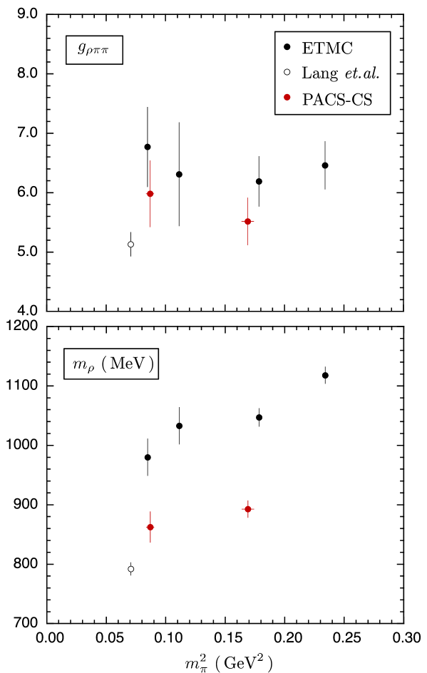
Figure 8: Comparison of our results (PACS-CS) obtained in $2+1$ flavor QCD with those by ETMC and Lang et al. in $2$ flavor QCD. Upper panel shows the effective coupling constant $g_{\rho\pi\pi}$ and lower is the resonance mass $m_{\rho}$. The systematic uncertainty for the determination of the lattice spacing is added to the statistical error in quadrature.

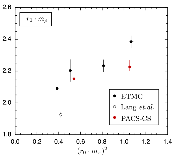
Figure 9: Comparison of our results (PACS-CS) with those by ETMC and Lang et al. for dimensionless value $r_{0}m_{\rho}$ as a function of $(r_{0}m_{\pi})^{2}$ with the Sommer scale $r_{0}$. The error of $r_{0}$ is added to the statistical error in quadrature.

Table 1: The ground and the first excited states with the isospin $(I,I_{z})=(1,0)$ for the irreducible representations considered in the present work, ignoring the hadron interactions. ${\bf P}$ is the total momentum, ${\rm g}$ is the rotational group in each momentum frame on the lattice and $\Gamma$ is the irreducible representation of the rotational group. The vectors in parentheses after $(\pi\pi)$ and $\rho$ refer to the momenta of the two pions and the $\rho$ meson in unit of $2\pi/L$. We use a notation $(\pi\pi)({\bf p}_{1})({\bf p}_{2})=\pi^{+}({\bf p}_{1})\pi^{-}({\bf p}_{2})-\pi^{-}({\bf p}_{1})\pi^{+}({\bf p}_{2})$ for the two-pion states. An index $j$ for the ${\bf T}_{1}^{-}$ representation takes $j=1,2,3$ and $k$ for the ${\bf E}^{-}$ takes $k=1,2$.

frame	${\bf P}L/(2\pi)$	g	$\Gamma$
CMF	$(0,0,0)$	$O_{h}$	${\bf T}_{1}^{-}$	$\rho_{j}({\bf 0})$	$(\pi\pi)({\bf e}_{j})(-{\bf e}_{j})$
MF1	$(0,0,1)$	$D_{4h}$	${\bf E}^{-}$	$\rho_{k}(0,0,1)$	$(\pi\pi)({\bf e}_{3}+{\bf e}_{k})(-{\bf e}_{k})-(\pi\pi)({\bf e}_{3}-{\bf e}_{k})({\bf e}_{k})$
MF1	$(0,0,1)$	$D_{4h}$	${\bf A}_{2}^{-}$	$\rho_{3}(0,0,1)$	$(\pi\pi)(0,0,1)(0,0,0)$
MF2	$(1,1,0)$	$D_{2h}$	${\bf B}_{1}^{-}$	$(\rho_{1}+\rho_{2})(1,1,0)$	$(\pi\pi)(1,1,0)(0,0,0)$

Table 2: Results at $m_{\pi}=410\,{\rm MeV}$. ${\bf P}$ is the total momentum and $\Gamma$ is the irreducible representation of the rotational group on the lattice. $E$ is the energy extracted by fitting the time correlation function with the fitting range in a line of “Fit Range”. $\sqrt{s}$ is the invariant mass and $k$ is the scattering momentum, which are related by $\sqrt{s}=\sqrt{E^{2}-|{\bf P}|^{2}}=2\sqrt{k^{2}+m_{\pi}^{2}}$. $\delta(k)$ is the $P$-wave scattering phase shift given by the finite size formulas in (2). We use the value of the lattice spacing given in the previous work in Ref. conf:PACS-CS , $a=0.907(13)\,{\rm fm}$ ($1/a=2.176(31)\,{\rm GeV}$), to obtain the values in the physical unit, where the error of the lattice spacing is not included.

$am_{\pi}$	$0.18897(79)$
$m_{\pi}\,({\rm MeV})$	$411.2(1.7)$
frame	CMF	MF1	MF1		MF2
${\bf P}L/(2\pi)$	$(0,0,0)$	$(0,0,1)$	$(0,0,1)$		$(1,1,0)$
$\Gamma$	${\bf T}_{1}^{-}$	${\bf E}^{-}$	${\bf A}_{2}^{-}$		${\bf B}_{1}^{-}$
Fit Range	$23-36$	$23-36$	$24-30$	$24-30$	$24-30$	$24-30$
$aE$	$0.4200(49)$	$0.4622(53)$	$0.4426(24)$	$0.4774(27)$	$0.4891(30)$	$0.5364(60)$
$a\sqrt{s}$	$0.4200(49)$	$0.4184(58)$	$0.3967(27)$	$0.4352(30)$	$0.4027(37)$	$0.4589(70)$
$(ak)^{2}\,\,(\times 10^{-3})$	$8.4(1.1)$	$8.1(1.2)$	$3.63(41)$	$11.63(57)$	$4.83(80)$	$16.9(1.5)$
$\sqrt{s}\,({\rm MeV})$	$914(11)$	$911(13)$	$863.2(5.9)$	$946.9(6.4)$	$876.2(8.1)$	$999(15)$
$s\,({\rm GeV}^{2})$	$0.835(19)$	$0.829(23)$	$0.745(10)$	$0.897(12)$	$0.768(14)$	$0.997(30)$
$a^{2}k^{3}/\tan\delta/\sqrt{s}\,\,(\times 10^{-3})$	$-1.872(19)$	$-2.120(22)$	$5.79(85)$	$-15.5(1.7)$	$2.36(49)$	$-28(11)$
$k^{3}/\tan\delta/\sqrt{s}\,\,(\times 10^{-2}\,{\rm GeV^{2}})$	$-0.8865(88)$	$-1.004(11)$	$2.74(40)$	$-7.34(80)$	$1.11(23)$	$-13.0(5.2)$

Table 3: Same as Table 2 for $m_{\pi}=300\,{\rm MeV}$.

$am_{\pi}$	$0.1355(15)$
$m_{\pi}\,({\rm MeV})$	$294.9(3.3)$
frame	CMF	MF1	MF1		MF2
${\bf P}L/(2\pi)$	$(0,0,0)$	$(0,0,1)$	$(0,0,1)$		$(1,1,0)$
$\Gamma$	${\bf T}_{1}^{-}$	${\bf E}^{-}$	${\bf A}_{2}^{-}$		${\bf B}_{1}^{-}$
Fitting Range	$23-36$	$23-36$	$24-30$	$24-30$	$24-30$	$24-30$
$aE$	$0.400(13)$	$0.452(12)$	$0.3658(40)$	$0.4511(85)$	$0.4377(80)$	$0.492(18)$
$a\sqrt{s}$	$0.400(13)$	$0.407(13)$	$0.3086(47)$	$0.4061(95)$	$0.338(10)$	$0.406(22)$
$(ak)^{2}\,\,(\times 10^{-3})$	$21.7(2.5)$	$23.0(2.7)$	$5.45(59)$	$22.9(1.9)$	$10.3(1.9)$	$22.8(4.5)$
$\sqrt{s}\,({\rm MeV})$	$871(28)$	$885(29)$	$672(10)$	$884(21)$	$736(23)$	$883(48)$
$s\,({\rm GeV}^{2})$	$0.758(48)$	$0.783(50)$	$0.451(14)$	$0.781(37)$	$0.542(33)$	$0.780(84)$
$a^{2}k^{3}/\tan\delta/\sqrt{s}\,\,(\times 10^{-3})$	$2.1(1.9)$	$1.4(1.6)$	$25(11)$	$-6.60(97)$	$4.1(4.3)$	$-12.3(3.7)$
$k^{3}/\tan\delta/\sqrt{s}\,\,(\times 10^{-2}\,{\rm GeV}^{2})$	$1.00(90)$	$0.68(76)$	$12.0(5.4)$	$-3.13(46)$	$19(21)$	$-5.8(1.7)$

References

(1)
C. Jung,
PoS LATTICE2009, 002 (2009)
[arXiv:1001.0941 [hep-lat]];
C. Hoelbling,
PoS LATTICE2010, 011 (2010)
[arXiv:1102.0410 [hep-lat]].
(2)
S. Gottlieb, P.B. Mackenzie, H.B. Thacker and D. Weingarten,
Phys. Lett. B134, 346 (1984).
(7)
K. Rummukainen and S. Gottlieb,
Nucl. Phys. B450, 397 (1995)
[hep-lat/9503028].
(8)
ETMC Collaboration,
X. Feng, K. Jansen and D.B. Renner,
PoS LATTICE2010, 104 (2010)
[arXiv:1104.0058 [hep-lat]].
(9)
CP-PACS Collaboration,
S. Aoki et al.,
Phys. Rev. D76, 094506 (2007)
[arXiv:0708.3705 [hep-lat]].
(10)
ETMC Collaboration,
X. Feng, K. Jansen and D.B. Renner,
PoS LATTICE2009, 109 (2009)
[arXiv:0910.4871 [hep-lat]].
(11)
ETMC Collaboration,
X. Feng, K. Jansen and D.B. Renner,
Phys. Rev. D83, 094505 (2011)
[arXiv:1011.5288 [hep-lat]].
(12)
C.B. Lang, D. Mohler, S. Prelovsek and M. Vidmar,
Phys. Rev. D84, 054503 (2011)
[arXiv:1105.5636 [hep-lat]].
(13)
PACS-CS Collaboration,
S. Aoki et al.,
Phys. Rev. D79, 034503 (2009)
[arXiv:0807.1661 [hep-lat]].
(14)
QCDSF Collaboration,
M. Gockeler et al.,
PoS LATTICE2008, 136 (2008)
[arXiv:0810.5337 [hep-lat]].
(15)
BMW collaboration,
J. Frison et al.,
PoS LATTICE2010, 139 (2010)
[arXiv:1011.3413 [hep-lat]].
(16)
C. Morningstar, A. Bell, J. Bulava, J. Foley,
K.J. Juge, D. Lenkner and C.H. Wong,
arXiv:1103.2783 [hep-lat];
C. Morningstar, J. Bulava, J. Foley,
K.J. Juge, D. Lenkner, M. Peardon and C.H. Wong,
Phys. Rev. D83, 114505 (2011)
[arXiv:1104.3870 [hep-lat]].
(17)
PACS-CS Collaboration,
S. Aoki et al.,
PoS LATTICE2010, 108 (2010)
[arXiv:1011.1063 [hep-lat]].
(18)
A. Messiah,
Quantum mechanics,
Vols. I, II ( North-Holland, Amsterdam, 1965 ).
(19)
CP-PACS Collaboration,
T. Yamazaki et al.,
Phys. Rev. D70, 074513 (2004)
[hep-lat/0402025].
(20)
M. Lüscher and U. Wolff,
Nucl. Phys. B339, 222 (1990).
(21)
ALPHA Collaboration,
B. Blossier et al.,
J. High Energy Phys. 04 (2009) 094
[arXiv:0902.1265 [hep-lat]].
(22)
K. Nakamura et al. (Particle Data Group),
J. Phys. G 37, 075021 (2010)
(23)
ETMC Collaboration,
R. Baron et al.,
J. High Energy Phys. 08 (2010) 097
[arXiv:0911.5061 [hep-lat]].