• Detection Thresholds and Bias Correction in Polarized Intensity

  Samuel J. George^A, Jeroen M. Stil^A, and Ben W. Keller^{A
  A} Institute for Space Imaging Science & Department of Physics and Astronomy, The University of Calgary, 2500 University Drive NW, Calgary AB, T2N 1N4, Canada  Email: samuel@ras.ucalgary.ca
  

  Detection thresholds in polarized intensity and polarization bias correction are investigated for surveys where the polarization information is obtained from RM synthesis. Considering unresolved sources with a single rotation measure, a detection threshold of $8\sigma_{QU}$ applied to the Faraday spectrum will retrieve the RM with a false detection rate less than $10^{-4}$, but polarized intensity is more strongly biased than Ricean statistics suggest. For a detection threshold of $5\sigma_{QU}$, the false detection rate increases to $\sim 4\%$, depending also on $\lambda^{2}$ coverage and the extent of the Faraday spectrum. Non-Gaussian noise in Stokes $Q$ and $U$ due to imperfect imaging and calibration can be represented by a distribution that is the sum of a Gaussian and an exponential. The non-Gaussian wings of the noise distribution increase the false detection rate in polarized intensity by orders of magnitude. Monte-Carlo simulations assuming non-Gaussian noise in $Q$ and $U$, give false detection rates at $8\sigma_{QU}$ similar to Ricean false detection rates at $4.9\sigma_{QU}$.

  Keywords: polarization — methods: statistical — methods: data analysis

1 Introduction

Linear polarization of radio sources contains information on magnetic fields in these sources, and Faraday rotation of the plane of polarization provides information on the direction and magnitude of the magnetic field along the line of sight. As such, observations of linear polarization of radio sources provide the most widely applicable probe of cosmic magnetic fields on scales from galaxies to clusters of galaxies. Finding polarized sources in survey images and fitting their parameters forms the basis of this analysis.

Sources with detectable polarized emission are readily identified in images of total intensity. As a first approximation, source finding in polarization can be reduced to applying a suitable detection threshold to the polarized intensity at the location of every radio source identified in total intensity. In practice, source finding in polarization is more complicated because of two reasons. The first is related to resolved sources, and the second is related to Faraday rotation of the polarized emission.

Figure 1 shows a radio source from the National Radio Astronomy Observatory (NRAO) Very Large Array (VLA) Sky Survey (NVSS; Condon et al. 1998) that is slightly resolved in total intensity (white contours), with major axis $68$” in position angle $-72^{\circ}$. The polarized emission is shown in grey scales as Stokes $Q$ and $U$ images. The source has a component that is unresolved at the $45$” resolution of the NVSS. The unresolved component has a peak polarized intensity of $6$ mJy ($\sigma_{QU}$ = $0.35$ mJy), approximately twice the catalogued value derived from the polarized intensity at the fitted position of the source in total intensity. It is not clear which fraction of radio sources has different morphology in polarized intensity than in total intensity. Approximately $8$% of NVSS sources brighter than $10$ mJy outside the Galactic plane ($|b|>30^{\circ}$) has a fitted (i.e. before deconvolution) major axis size more than $1.5$ times the $45^{\prime\prime}$ (FWHM) size of the synthesized beam, and $2\%$ has a fitted major axis more than twice the beam size.

Resolved polarized sources have been treated in different ways in the literature. The NVSS catalog derived polarized intensity at the location of the fitted position in total intensity, and the listed polarized flux density (peak times Stokes $I$ solid angle) implicitly assumes a constant polarization angle over the source. Taylor et al. (2007) and Grant et al. (2010) fitted 2-dimensional Gaussians to sources in polarized intensity. Subrahmanyan et al. (2010) integrated Stokes $Q$ and $U$ over the solid angle of the source defined in a low-resolution total intensity image, and catalogued each polarized source as if it were unresolved.

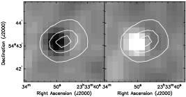
Figure 1: A radio source that is resolved in total intensity, with one-sided polarization. Grey scales show Stokes $Q$ and $U$ from the NVSS with contours of total intensity at $3$, $30$, and $60$ mJy. The grey scales range from $-3$ mJy (black) to $+3$ mJy (white).

The second complication for source finding in linear polarization is presented by Faraday rotation, even if the source is unresolved. Faraday rotation rotates the polarization angle $\Psi$ by an amount proportional to $\lambda^{2}$ for a simple Faraday thin source, and in a more complicated manner e.g. if synchrotron emission and Faraday rotation both occur in the same volume. Differential Faraday rotation over the observed frequency range leads to depolarization, thus introducing a selection effect against sources with strong Faraday rotation (Stil & Taylor 2007, for the NVSS). Multifrequency observations allow Rotation Measure (RM) Synthesis Burn (1966); Brentjens & De Bruyn (2005) to solve for the unknown Faraday depth, polarized intensity, and polarization angle simultaneously. The source is typically identified by the maximum value in the Faraday spectrum, e.g. through the RM clean algorithm (Heald 2009).

Following Brentjens & De Bruyn (2005) the Faraday depth $\phi$ is defined as

$$\phi\left(\vec{r}\right)=0.81\int_{0}^{x}\vec{B_{||}}n_{e}\cdot\mathrm{d}\vec{r}\ \mbox{rad}\ \mbox{m}^{-2},$$ (1)

where $\vec{B_{||}}$ is the line of sight magnetic field component, $n_{e}$ is the thermal electron density, $\mathrm{d}\vec{r}$ is an infinitesimal path length, with the integral taken from the observer to the point $x$.

The complex polarized intensity $\mathcal{P}\left(\lambda^{2}\right)=Q+iU$ is the Fourier transform of the Faraday dispersion function $F(\phi)$,

$$P\left(\lambda^{2}\right)=\int_{-\infty}^{\infty}F(\phi)e^{2i\phi\lambda^{2}}d\phi.$$ (2)

The Faraday rotation measure $RM$ is defined as the slope of a polarization angle $\Psi$ versus $\lambda^{2}$ plot:

$$RM\left(\lambda\right)=\frac{d\Psi}{d(\lambda^{2})}$$ (3)

where

$$\Psi=\frac{1}{2}\tan^{-1}\frac{U}{Q}.$$ (4)

Once a polarized source has been detected, the observed polarized intensity $p=\sqrt{Q^{2}+U^{2}}$ must be corrected for polarization bias. Since $p$ is a positive-definite quantity, the noise in Stokes $Q$ and $U$ results in a positive value for $p$ even if no signal is present. The statistics of $p$ with a signal $p_{0}$ and noise $\sigma_{QU}$ is given by the Rice distribution (Rice 1945). Estimators of the true polarized flux density $p_{0}$ from the observed polarized flux density $p$ based on this distribution have been discussed by a number of authors (Simmons & Stewart 1985; Vaillancourt 2006). The Rice distribution assumes Gaussian noise in Stokes $Q$ and $U$. Real surveys of the sky may have non-Gaussian tails to the noise distribution resulting from imperfect imaging and calibration. In this paper we investigate the detection statistics in polarized intensity and polarization bias correction for polarized intensity determined from RM synthesis and in the presence of non-Gaussian noise in Stokes $Q$ and $U$.

Future radio polarization surveys such as the Galactic Arecibo L-band Feed Array Continuum Transit Survey (GALFACTS; Taylor & Salter 2010) and the Polarization Sky Survey of the Universe’s Magnetism
(POSSUM; Gaensler et al. 2010) are wide band, multifrequency surveys that require revision of detection threshold and polarization bias correction.

2 RM Synthesis simulations

Table 1: False detection rates in simulated Faraday spectra. (1) Ratio of true polarized signal to the noise in Stokes $Q$ and $U$. (2) Percentage of simulated spectra with $|~{}\phi-\phi_{0}~{}|>50\ \mbox{rad\,m${}^{-2}$}$. No false detections were found in the $3.33\times 10^{4}$ $8\sigma_{QU}$ simulated spectra. These percentages depend in part on the Faraday depth range considered, and the width of the RM spread function.

$p_{0}/\sigma_{QU}$	% False Detection
(1)	(2)
2.0	73.9
3.0	43.9
4.0	16.7
5.0	3.6
6.0	0.43
7.0	0.033
8.0	…

RM synthesis was performed on simulated data for sources with signal to noise ratio $p_{0}/\sigma_{QU}$ ranging from $0$ to $15$. Each realization contained a source with the prescribed polarized signal and random polarization angle at the reference frequency, $1400$ MHz. Stokes $Q$ and $U$ values were calculated assuming a Faraday depth of $150$ rad m^-2  for $N_{\rm chan}=1024$ frequency channels between $1000$ MHz and $1400$ MHz. Gaussian noise with standard deviation $\sigma=\sqrt{N_{\rm chan}}$ was added to each channel, resulting in a standard deviation $\sigma_{QU}=1$ for the noise in Stokes $Q$ and $U$ after averaging over all channels. RM synthesis was then performed on the synthetic spectrum of complex polarization. The effect of spectral index $\alpha$ ($S_{\nu}\sim\nu^{\alpha}$), assuming that the percentage polarization is constant across the band, was investigated with separate simulations for $\alpha=0$ and $\alpha=-0.75$. For each combination of $p_{0}/\sigma_{QU}$ and $\alpha$, $33\,\,300$ simulated Faraday spectra were analyzed.

Figure 2 shows two simulated Faraday spectra with and without noise. The noiseless spectra show the RM spread function with its side lobes. The near side lobes of the RM spread function raise the probability of a false peak at the wrong Faraday depth, resulting in stronger wings in the error function of the Faraday depth when the signal to noise ratio is low. As the Faraday depth of the source is not known a priori, the location of the peak in the Faraday spectrum is catalogued as the Faraday depth of the source, and the amplitude of the peak as the observed polarized intensity $p_{\rm max}$. We also extract the polarized intensity $p$ at the input Faraday depth, because of the expectation that the Rice distribution with noise $\sigma_{QU}=1$ applies to $p$, not necessarily to $p_{\rm max}$.

Table 2: Expectation values of polarized intensity and bias correction. (1) Spectral index ($S_{\nu}\sim\nu^{\alpha}$). (2) Input polarized intensity at centre of the band in units of $\sigma_{QU}$, and constant percentage polarization across the frequency band. (3) Effective polarized intensity defined in Equation 2. (4) Polarized intensity in the Faraday profile at the input Faraday depth ($150\ \mbox{rad\,m${}^{-2}$}$). This quantity is not known for real sources. (5) Maximum polarized intensity taken over all Faraday depth values. (6) Estimator of $p_{0,eff}$ taking polarized intensity from column 4, according to $\hat{p}_{\phi_{0}}=\sqrt{p_{\phi_{0}}^{2}-\sigma_{QU}^{2}}$. This quantity is not known for real sources. (7) Estimator of $p_{0,eff}$ taking polarized intensity from column 5, according to $\hat{p}_{0}=\sqrt{p_{\rm max}^{2}-2.3\sigma_{QU}^{2}}$.

$\alpha$	$p_{0}/\sigma_{QU}$	$p_{0,eff}/\sigma_{QU}$	$p_{\phi_{0}}/\sigma_{QU}$	$p_{\rm max}/\sigma_{QU}$	$\hat{p}_{\phi_{0}}/\sigma_{QU}$	$\hat{p}_{0}/\sigma_{QU}$
(1)	(2)	(3)	(4)	(5)	(6)	(7)
0.00	4.000	4.000	4.139	4.384	4.020	4.114
0.00	5.000	5.000	5.106	5.237	5.009	5.012
0.00	6.000	6.000	6.092	6.188	6.011	5.999
0.00	7.000	7.000	7.076	7.156	7.006	6.994
0.00	8.000	8.000	8.072	8.142	8.011	8.000
0.00	9.000	9.000	9.070	9.130	9.015	9.004
0.00	10.000	10.000	10.053	10.107	10.003	9.993
0.00	15.000	15.000	15.027	15.063	14.994	14.986
$-$0.75	4.000	4.110	4.246	4.467	4.130	4.202
$-$0.75	5.000	5.138	5.244	5.365	5.150	5.147
$-$0.75	6.000	6.165	6.255	6.345	6.175	6.161
$-$0.75	7.000	7.193	7.272	7.347	7.204	7.188
$-$0.75	8.000	8.221	8.288	8.353	8.227	8.215
$-$0.75	9.000	9.248	9.305	9.362	9.251	9.238
$-$0.75	10.000	10.276	10.332	10.383	10.284	10.272
$-$0.75	15.000	15.413	15.444	15.478	15.412	15.403

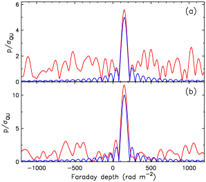
Figure 2: Faraday spectra of simulated sources with signal to noise ratio $p_{0}/\sigma_{QU}=5$ (a) and $10$ (b), both with Faraday depth of $150$ rad m^-2. The red curves represent the spectrum with noise, while the blue curves show the corresponding spectrum without noise.

Figure 3 shows the distribution of Faraday depths derived from the simulations for $p/\sigma_{QU}=2$ and $4$ and $\alpha=0$. While each Faraday profile contains a source with the input $\phi_{0}$ $=150\ \mbox{rad\,m${}^{-2}$}$, the uniform distribution of Faraday depths at low signal to noise ratios represents spurious peaks in excess of the actual source. The effect of these false detections is twofold: expectation value of the polarized intensity approximates a nearly constant value for $p_{0}/\sigma_{QU}<3$, and the error distribution in Faraday depth becomes significantly non-Gaussian. Table 1 lists false detection rates as a function of signal to noise ratio. In the range $3\leq p_{0}/\sigma_{QU}\leq 8$ the false detection rate drops to below $10^{-4}$, and the error distribution of Faraday depth becomes approximately Gaussian.

Figure 3: Distribution of Faraday depths, with input $\phi_{0}$ $=150\ \mbox{rad\,m${}^{-2}$}$, derived from simulations with (a) $p/\sigma_{QU}=2$ and (b) $p/\sigma_{QU}=4$.

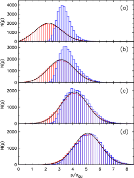
Figure 4: Distribution of polarized intensity derived from simulated Faraday spectra. Signal to noise $p_{0}/\sigma_{QU}=2,3,4,5$ for panels (a)-(d) respectively. The red histograms represent values of $p$ at the actual Faraday depth of the source, and the black curves show the Rice distribution for the assumed value of $p_{0}/\sigma_{QU}$. The blue histograms represent polarized intensity at the peak of the Faraday spectrum.

Figure 4 shows the distributions of polarized intensity derived from the simulations, along with curves representing the Rice distribution for $p_{0}/\sigma_{QU}=$ $2$, $3$, $4$, and $5$. The red histogram shows the polarized intensity $p_{\phi_{0}}$ at the actual Faraday depth of the source, demonstrating the Ricean statistics for this quantity. In reality, we do not know the actual Faraday depth of the source, but solve for this by finding $p_{\rm max}$, defined as the peak of the Faraday spectrum. The distributions of $p_{\rm max}$ are shown by the blue histograms in Figure 4. At any signal to noise ratio, the distribution of $p_{\rm max}$ is shifted to higher $p$ with respect to the Rice distribution, adding to the polarization bias. This additional bias is closely related to the fitting bias for fitting the flux density of a source discussed by Condon et al. (1998). The magnitude of this bias is similar to the well-known polarization bias.

For $p_{0}/\sigma_{QU}<5$, the distribution of $p_{\rm max}$ is skewed with respect to the Rice distribution. The distribution of $p_{\rm max}$ can be approximated by the distribution of the maximum of $N-1$ independent draws from the Rice distribution with no signal, and $1$ draw from the Rice distribution with the seeded signal $p_{0}$, where $N$ is the ratio of the range of the Faraday spectrum to the FWHM width of the RM spread function. The sidelobes of the RM spread function increase the false detection rate, so this explanation can only be an approximation. The difference between the distribution of $p_{\rm max}$ and the Rice distribution at low signal to noise depends on the range of the Faraday spectrum. At high signal to noise ratios, the maximum is always associated with the source, and the fitting bias is independent of the range of the RM spectrum.

Table 2 lists expectation values of polarized intensity for flat spectrum sources and steep spectrum sources at a range of signal to noise ratios in polarized intensity. Column 6 lists the estimated true polarized intensity using $\hat{p}^{\phantom{1}}_{\phi_{0}}=\sqrt{p_{\phi_{0}}^{2}-\sigma_{QU}^{2}}$. Though this is not measurable in real data, the correspondence between column 6 and column 2 reflects the Ricean statistics of $p_{\phi_{0}}$ illustrated in Figure 4. The bias in $p_{\rm max}$ measured from real data is approximately twice as large as in $p_{\phi_{0}}$. The polarization bias correction can be adjusted to correct for the additional bias associated with the uncertainty in RM. The estimator

$$\hat{p}_{0}=\sqrt{p^{2}-2.3\sigma_{QU}^{2}}$$ (5)

for $p/\sigma_{QU}>4$ provides accurate estimates of $p_{0}$.

This work suggests that a detection threshold of $p_{0}/\sigma_{QU}>8$ should be applied for the derivation of Faraday depth, in order to obtain a well-behaved error function of Faraday depth. Polarized intensity can be estimated for sources with $p_{0}/\sigma_{QU}>4$, depending on the desired level of acceptable false detections.

In the case where $\alpha\neq 0$, Brentjens & De Bruyn (2005) recommend dividing by the total brightness as a function of frequency. This may work well for bright sources, but not for faint sources, or diffuse polarized emission. In our experiments, we find that the Faraday depth derived for sources with $\alpha=-0.75$ was not significantly different from sources with $\alpha=0$, but the polarized intensity after polarization bias correction is given by $p_{eff}$ defined as

$$p_{eff}={{\int pd\lambda^{2}}\over{\int d\lambda^{2}}},$$ (6)

where the integral is evaluated over the wavelength range of the data. The penalty of not dividing by total intensity creates a spectral-index dependent bias in polarization that is larger than the effects discussed previously.

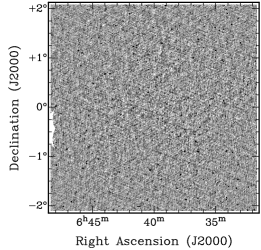
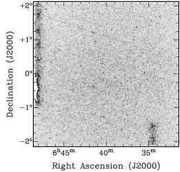
Figure 5: Example of one of the $4^{\circ}\times 4^{\circ}$ fields in (top) total and (bottom) polarized intensity, illustrating the effects of missing fields on the noise.

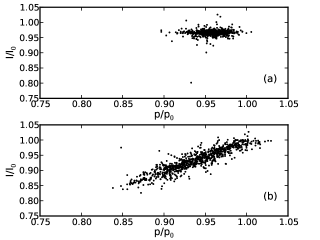
Figure 6: Comparison of the ratio of peak values ($I$ and $p$) retrieved from the image and the input values ($I_{0}$ and $p_{0}$) for sources with $p>20$ mJy. (a) shows peak fluxes determined from fitting with SAD, (b) shows the nearest pixel value.

3 Simulated Sky Survey

Sky simulations with sensitivity and angular resolution similar to the NVSS over an area of $2.33$ sr covering $478$ $4^{\circ}\times 4^{\circ}$ fields were constructed to test source finding and stacking algorithms. Figure 5 shows a simulated image in total intensity and polarized intensity. The images were constructed with source density and noise level similar to the NVSS polarization images. The images were built up by seeding sources at random positions in the image plane. Each source consists of a VLA snapshot antenna pattern scaled to the assumed clean limit plus a two dimensional Gaussian representing the restored clean components. The sidelobes of the antenna patterns from different sources add up incoherently simulating incomplete cleaning. The Gaussian noise divided by the sensitivity pattern of the NVSS mosaics was added to the Stokes $I$, $Q$ and $U$ images. The noise level in Stokes $I$ is $2$ mJy, whilst $Q$ and $U$ is $0.4$ mJy. Images with missing fields were included to simulate survey edges. The distribution of polarized fraction of sources followed the distribution derived by Beck & Gaensler (2004) for NVSS source brighter than $80$ mJy. The images only contain unresolved sources and the resolution of the images is $45$” with a pixel size of $15$”.

The images were searched for sources in total intensity and polarized intensity with the AIPS (Astronomical Image Processing System) source finder SAD (Search and Destroy), with a detection threshold of $5$ mJy. The recovered sources were matched with the input source catalogue. Only sources that matched within $60^{\prime\prime}$ were considered for further analysis. For sources with $I>50$ mJy the standard deviations in right ascension and declination were $1.47$” and $1.46$” respectively.

The peak flux in both total and polarized intensity is found in two ways. By using SAD to find and fit the sources and by extracting the nearest pixel value for $I$ and $p$. The nearest pixel values are considered because RM synthesis is done per pixel. Figure 6 compares the fitted peak and the nearest pixel values with the input catalog for both total intensity and polarized intensity for sources with $p>20$ mJy. The fitted peak values underestimate the input values by a few percent, but the solid angle of the source from the fits is slightly overestimated so that the integrated flux density is retrieved from the catalogue. The nearest pixel intensities underestimate the true intensity by up to 15%, approximately along the line of constant $p/I$. The error in the fitted position of the source is much smaller than a pixel, so the uncertainty in the position of the source in total intensity does not introduce a significant error in the estimation of $p$. RM synthesis on the brightest pixel would introduce a systematic error in polarized intensity comparable to that shown in Figure 6b. Figure 6 suggests that source finding in the image plane after RM synthesis is required to obtain polarized flux densities with an accuracy better than $\sim 10\%$.

4 Non-Gaussian noise in $Q$/$U$

The statistics of polarized intensity are usually described by the Rice distribution that assumes Gaussian noise in $Q$ and $U$. Imperfect imaging and calibration result in images that do not achieve the theoretical noise levels. The actual noise distribution has strong wings above Gaussian noise.

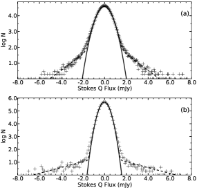
Figure 7: Histograms of the noise for Stokes $Q$ images for (a) the simulated images (b) the NVSS. The fitted curves are (solid) a Gaussian fit and (dashed) the summation of a Gaussian and an exponential.

Figure 7 shows the noise distribution for both the simulated and the NVSS images. Sources identified in total intensity were masked out of the Stokes $Q$ and $U$ images leaving pixels that are free of detectable polarized emission. For determining the noise statistics, areas near missing fields were not considered. The solid curves in Figure 7 represent Gaussians with standard deviation equal to the $rms$ of empty areas in the images avoiding sources. The non-Gaussian wings in $Q$ and $U$ emerging above the $2\sigma_{QU}$ level are related to the striping visible in Figure 5. In both cases a Gaussian does not adequately represent the wings of the noise distribution. A better solution is the sum of a Gaussian and an exponential,

$$F(x)=Ae^{-x^{2}/2\sigma^{2}}+Be^{-C|x|},$$ (7)

with $A$, $B$ and $C$ determined from fitting. The parameters of the fit for the Stokes $Q$ simulated images are: $A=0.95341$, $B=0.00659$, $C=1.08135$ and $\sigma=0.44327$.

To investigate the impact on false detection rate in polarized intensity, Monte-Carlo simulations of polarized intensity using the noise distribution from Equation 7 and $p_{0}=0$ were done. First a $Q$ value was drawn. In principle $Q$ values were drawn independently from $U$ values. However, if the $|Q|$ was larger than a $2\sigma_{QU}$ threshold, $U$ values were drawn until the $|U|$ was also larger than the $2\sigma_{QU}$. This procedure acknowledges that in real data residual sidelobes in $Q$ probably also exist in $U$.

Figure 8 shows the false detection rate in polarized intensity for Gaussian and non-Gaussian noise in Stokes $Q$ and $U$ and Table 3 lists false detection rates for a range of detection thresholds $p_{lim}$ in polarized intensity. The details of Figure 8 depend on the dynamic range of the $Q$ and $U$ images and will be different for every survey. The non-Gaussian wings in $Q$ and $U$ increase the false detection rate by orders of magnitude. In the simulations an $8\sigma$ detection threshold yields the same false detection rate as a $4.9\sigma$ detection threshold for Ricean statistics.

Polarized source finding should apply a detection threshold that is derived from the actual noise distribution in $Q$ and $U$ of a dynamic range limited survey. We found no significant effect on the bias correction from the non-Gaussian wings.

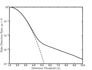
Figure 8: False detection rates determined from Monte-Carlo simulations of the noise distribution for $p_{0}=0$. The dashed curve represents a Gaussian fit to the noise and the solid curve uses the sum of the Gaussian and exponential noise function.

Table 3: False detection rates of polarized intensity for Gaussian (i.e. Ricean) and non-Gaussian (i.e. non-Ricean) noise in Stokes $Q$ and $U$.

$p_{lim}/\sigma_{QU}$	Ricean	Non-Ricean
3.0	$1.36\times 10^{-1}$	$1.41\times 10^{-1}$
3.5	$4.43\times 10^{-2}$	$4.88\times 10^{-2}$
4.0	$1.13\times 10^{-2}$	$1.51\times 10^{-2}$
4.5	$2.23\times 10^{-3}$	$5.34\times 10^{-3}$
5.0	$3.35\times 10^{-4}$	$2.82\times 10^{-3}$
5.5	$3.85\times 10^{-5}$	$2.00\times 10^{-3}$
6.0	$2.90\times 10^{-6}$	$1.54\times 10^{-3}$
6.5	$3.00\times 10^{-7}$	$1.20\times 10^{-3}$
7.0	-	$9.43\times 10^{-4}$
7.5	-	$7.42\times 10^{-4}$
8.0	-	$5.84\times 10^{-4}$
8.5	-	$4.60\times 10^{-4}$
9.0	-	$3.58\times 10^{-4}$
9.5	-	$2.73\times 10^{-4}$
10.0	-	$2.03\times 10^{-4}$

5 Summary & Conclusions

The uncertainty in the Faraday depth of the source introduces a stronger bias in polarized intensity than just the well known polarization bias. At low signal to noise the false detection rate is greatly enhanced, while at higher signal to noise ($p>4\sigma_{QU}$) an effective estimator for the true polarized intensity is $\hat{p}_{0}=\sqrt{p^{2}-2.3\sigma_{QU}^{2}}$.

RM synthesis on the pixel nearest to the fitted position of total intensity introduces a systematic error that underestimates the polarized intensity by up to $15\%$. Source fitting in polarized intensity provides a more accurate result, even for the unresolved sources considered in this paper.

Non-Gaussian wings of the noise distribution in Stokes $Q$ and $U$ significantly increase the rate of false detection in polarized intensity by orders of magnitude. False detection rates at $8\sigma_{QU}$ similar to Ricean false detection rates at $4.9\sigma_{QU}$.

References

- Beck & Gaensler (2004) Beck, R., & Gaensler, B. M., 2004, New Astronomy Reviews, 48, 1289
- Brentjens & De Bruyn (2005) Brentjens, M. A., & De Bruyn, A. G. 2005, A&A 441, 1217
- Burn (1966) Burn, B. J. 1966, MNRAS, 133, 67
- Condon et al. (1998) Condon, J. J., Cotton, W. D., Greisen, E. W., Yin, Q. F., Perley, R. A., Taylor, G. B., & Broderick, J. J. 1998, AJ, 115, 1693
- Gaensler et al. (2010) Gaensler, B. M., Landecker, T. L., Taylor, A. R., POSSUM Collaboration, 2010, BAAS, 41, 515
- Grant et al. (2010) Grant, J. K., Taylor, A. R., Stil, J. M., Landecker, T. L., Kothes, R., Ransom, R. R., Scott, D., 2010, ApJ, 714, 1689
- Heald (2009) Heald, G., 2009, IAUS, 259, 591
- Rice (1945) Rice, S. O. 1945, Bell Syst. Tech. J., 24, 46
- Simmons & Stewart (1985) Simmons, J. F. L., & Stewart, B. G. 1985, A&A, 142, 100
- Stil & Taylor (2007) Stil, J M., Taylor, A. R., 2007, ApJ, 663, L21
- Subrahmanyan et al. (2010) Subrahmanyan, R., Ekers, R. D., Saripalli, L., Sadler, E. M., 2010, MNRAS, 402, 2792
- Taylor et al. (2007) Taylor, A. R., Stil, J. M., Grant, J. K., Landecker, T. L., Kothes, R., Reid, R. I., Gray, A. D., Scott, D., Martin, P. G., Boothroyd, A. I., Joncas, G., Lockman, F. J., English, J., Sajina, A., Bond, J. R. 2007, ApJ, 666, 201
- Taylor & Salter (2010) Taylor, A. R., Salter, C. J., 2010, Proceedings of the Conference ”The Dynamic ISM: A Celebration of the Canadian Galactic Plane Survey”, ASP Conference Series
- Vaillancourt (2006) Vaillancourt, J. E. 2006, PASP, 118, 1340