The su($n$) WZNW fusion ring as integrable model: a new algorithm to compute fusion coefficients

Abstract

This is a proceedings article reviewing a recent combinatorial construction of the $\widehat{\mathfrak{su}}(n)_{k}$ WZNW fusion ring by C. Stroppel and the author. It contains one novel aspect: the explicit derivation of an algorithm for the computation of fusion coefficients different from the Kac-Walton formula. The discussion is presented from the point of view of a vertex model in statistical mechanics whose partition function generates the fusion coefficients. The statistical model can be shown to be integrable by linking its transfer matrix to a particular solution of the Yang-Baxter equation. This transfer matrix can be identified with the generating function of an (infinite) set of polynomials in a noncommutative alphabet: the generators of the local affine plactic algebra. The latter is a generalisation of the plactic algebra occurring in the context of the Robinson-Schensted correspondence. One can define analogues of Schur polynomials in this noncommutative alphabet which become identical to the fusion matrices when represented as endomorphisms over the state space of the integrable model. Crucial is the construction of an eigenbasis, the Bethe vectors, which are the idempotents of the fusion algebra.

1 Introduction

Wess-Zumino-Novikov-Witten (WZNW) models are an important class of conformal field theories (CFT) distinguished by their Lie algebraic symmetry. Due to this symmetry the primary fields of WZNW theories are in one-to-one correspondence with the integrable highest weight representations of an affine Lie algebra; see e.g. the text book [4] for details and references. Consider the $\widehat{\mathfrak{su}}(n)_{k}$ WZNW model, then the set of all dominant integral weights of level $k\in\mathbb{Z}_{\geq 0}$ is given by

(1) $$P_{k}^{+}=\left\{\hat{\lambda}=\sum_{i=1}^{n}m_{i}\hat{\omega}_{i}\;\left|\;\sum_{i=1}^{n}m_{i}=k\right.\!,\;m_{i}\in\mathbb{Z}_{\geq 0}\right\}$$

where the $\hat{\omega}_{i}$’s denote the fundamental affine weights of the affine Lie algebra $\widehat{\mathfrak{su}}(n)$; see e.g. [13] for details. Note that we use the label $n$ instead of $0$ for the affine node. In what follows it will be convenient to identify elements in the set $P_{k}^{+}$ with the partitions $\mathcal{P}_{\leq n-1,k}$ whose Young diagram fits into a bounding box of height $n-1$ and width $k$. Namely, define a bijection $P_{k}^{+}\rightarrow\mathcal{P}_{\leq n-1,k}$ by setting

(2) $$\hat{\lambda}\mapsto\lambda=(\lambda_{1},\ldots,\lambda_{n-1})\quad\text{with}\quad\lambda_{i}-\lambda_{i+1}=m_{i}~{},$$

where $m_{i}$ is the so-called Dynkin label, i.e. the coefficient of the $i^{\text{th}}$ fundamental weight in (1). Vice versa, given a partition $\lambda\in\mathcal{P}_{\leq n-1,k}$ we shall denote by $\hat{\lambda}$ the corresponding affine weight in $P_{k}^{+}$.

Since the set of dominant integral weights at fixed level $k$ has cardinality $|P_{k}^{+}|=\binom{n+k-1}{k}$, WZNW models are so-called rational conformal field theories, i.e. they have a finite set of primary fields from which all other fields can be generated. An important ingredient in the description of rational conformal field theories is the concept of fusion: in physics terminology one considers the operator product expansion of two primary fields. While this can be made mathematically precise in the context of vertex operator algebras and the fusion process can be identified with the product in the Grothendieck ring of an abelian braided monoidal category in the context of tilting modules of quantum groups, we will not use this mathematical framework here.

Consider the free abelian group (with respect to addition) generated by $P_{k}^{+}$ and introduce the so-called fusion product

(3) $$\hat{\lambda}\ast\hat{\mu}=\sum_{\hat{\nu}\in P_{k}^{+}}\mathcal{N}_{\hat{\lambda}\hat{\mu}}^{(k)\hat{\nu}}\hat{\nu},$$

by defining the structure constants $\mathcal{N}_{\hat{\lambda}\hat{\mu}}^{(k)\hat{\nu}}\in\mathbb{Z}_{\geq 0}$, called fusion coefficients, via the celebrated Verlinde formula [19]

(4) $$\mathcal{N}_{\hat{\lambda}\hat{\mu}}^{(k)\hat{\nu}}=\sum_{\hat{\sigma}\in P_{k}^{+}}\frac{S_{\hat{\lambda}\hat{\sigma}}S_{\hat{\mu}\hat{\sigma}}S_{\hat{\nu}\hat{\sigma}}^{-1}}{S_{\hat{\emptyset}\hat{\sigma}}}\;.$$

Here $\hat{\emptyset}$ denotes the weight corresponding to the empty partition and $S$ is the modular $S$-matrix describing the modular transformation $\tau\rightarrow-\tau^{-1}$ of affine characters. Among other properties it enjoys unitarity $\bar{S}_{\hat{\nu}\hat{\sigma}}=S_{\hat{\nu}\hat{\sigma}}^{-1}$ and crossing symmetry $\bar{S}_{\hat{\lambda}\hat{\sigma}}=S_{\hat{\lambda}^{\ast}\hat{\sigma}},$ where $\hat{\lambda}^{\ast}$ is the dual weight obtained by taking the complement of $\lambda$ in the $(n-1)\times k$ bounding box and then deleting all $n$-columns, $\lambda^{\ast}=(\lambda_{1},\lambda_{1}-\lambda_{n-1},\lambda_{1}-\lambda_{n-2},\ldots,\lambda_{1}-\lambda_{2})$.

For WZNW models the explicit expression for $S$ is known: the Kac-Peterson formula [14] states $S$ in terms of the Weyl group $W$ and specialises for $\widehat{\mathfrak{su}}(n)$ to the expression

(5) $$S_{\hat{\lambda}\hat{\sigma}}=\frac{e^{i\pi n(n-1)/4}}{\sqrt{n(k+n)^{n-1}}}\sum_{w\in W}(-1)^{\ell(w)}e^{-\frac{2\pi i}{k+n}(\sigma+\rho,w(\lambda+\rho))}\;,$$

where $\rho$ is the Weyl vector and $\lambda,\sigma$ denote the finite, non-affine weights corresponding to $\hat{\lambda},\hat{\sigma}$. From this formula it is by no means obvious that the fusion coefficients (4) are non-negative integers, however they have been identified with certain dimensions or multiplicities in various different contexts as e.g. discussed in [9] (for references see loc. cit.): dimensions of spaces of conformal blocks of 3-point functions, so-called moduli spaces of generalised $\theta$-functions; outer multiplicities of truncated tensor products of tilting modules of quantum groups at roots of unity; Littlewood-Richardson coefficients of Hecke algebras at roots of unity; dimensions of local states in restricted-solid-on-solid models. In fact, (3) defines a unital, commutative ring over the integers $\mathbb{Z}$, which we shall refer to as the $\widehat{\mathfrak{su}}(n)$ fusion ring at level k, denoted by $\mathcal{F}_{n,k}$, and to the corresponding unital, commutative and associative algebra $\mathcal{F}_{n,k}^{\mathbb{C}}\mathbb{=\mathcal{F}}_{n,k}\mathbb{\otimes}_{\mathbb{Z}}\mathbb{C}$ as fusion or Verlinde algebra.

This article aims to give a non-technical account of the main findings in [15] and [16] regarding the $\widehat{\mathfrak{su}}(n)$ fusion ring. For proofs the reader is referred to the mentioned papers. Sections 2 and 3 are largely a summary of previous results reviewing the definition of an integrable statistical mechanics model which generates the fusion ring. It is convenient to describe the statistical model and its lattice configurations using non-intersecting paths, since this allows for instance a non-technical definition of the transfer matrix. However, it needs to be stressed that at the moment the path picture is not used to give combinatorial proofs, instead the discussion is algebraic and employs the solution to the Yang-Baxter equation given in [16]. However, we present one result, Corollary 2.3, which relates the counting of non-intersecting paths on the cylinder to a sum over fusion coefficients. We also make contact with the phase model of Bogoliubov, Izergin and Kitanine [2] where closely related algebraic structures have been discussed. Section 4 states a detailed derivation of the new algorithm to compute fusion coefficients. First a review of the Bethe ansatz equations is given by highlighting how they are connected to a fusion potential. The latter differs from the familiar fusion potential of Gepner [7] and the algorithm therefore yields expressions for fusion coefficients in terms of Littlewood-Richardson coefficients which differ from the ones obtained via the celebrated Kac-Walton formula [13] [20]; compare also with the work of Goodman and Wenzl [10]. Section 5 stresses that the Bethe vectors constructed via the quantum inverse scattering method can be identified with the idempotents of the fusion ring. The proof of this result has been given before [15] but their role has not been emphasized. The modular S-matrix is the transition matrix from the basis of integrable weights to the basis of Bethe vectors and, hence, can be expressed in terms of the generators of a Yang-Baxter algebra. We also present a new perspective on the affine plactic Schur polynomials which are defined in terms of the transfer matrix via a determinant formula: they constitute the set of conserved quantities of the integrable model and hence should be seen as the quantum analogue of a spectral curve. In the present model this quantum spectral curve coincides with the collection of $\widehat{\mathfrak{su}}(n)_{k}$ fusion rings for $k\in\mathbb{Z}_{\geq 0}$. We conclude with some practical applications, recursion formulae for fusion coefficients at different level. The last section discusses how the findings summarised here might generalise to a wider class of integrable models.

2 Fusion coefficients from statistical mechanics

We start by defining a statistical vertex model which is obtained in the crystal limit of $U_{q}\widehat{\mathfrak{su}}(2)$; see [16]. Consider a $n\times(n-1)$ square lattice with quasi-periodic boundary conditions in the horizontal direction, i.e. a square lattice on a cylinder with $n-1$ rows. On the edges of the square lattice live statistical variables $m\in\mathbb{Z}_{\mathbb{\geq}0}$, which we will identify with the Dynkin labels of dominant integrable weights below. To each lattice configuration we assign a “Boltzmann weight” in $\mathbb{C}[z][x_{1},\ldots,x_{n-1}]$ by taking the product over (local) vertex configurations.

Label the statistical variables $a,b,c,d\in\mathbb{Z}_{\mathbb{\geq}0}$ sitting on the edges of a vertex in the $i^{\text{th}}$ lattice row as shown in Figure 1, then we assign to it the weight (compare with [16])

(6) $$\mathcal{R}_{c,d}^{a,b}(x_{i})=\left\{\begin{array}[]{cc}x_{i}^{a},&d=a+b-c,\;b\geq c\\ 0,&\text{else}\end{array}\right.\;.$$

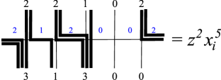
Figure 3: An example for $n=5$ and $k=7$ of a row configuration and its ”statistical weight”, which is obtained by counting the horizontal edges of paths. Outer edges are identified and for each a power of $z$ is added.

It is convenient to describe the vertex configurations in terms of non-intersecting paths, so-called $\infty$-friendly walkers; compare with [8, 11, 12]. In Figure 1 $b$ walkers are entering the vertex from above turning to the right, at which point a contingent of them of size $b-c$ chooses to defect. The defectors then join another group of $a$ walkers coming from the left. The Boltzmann weight of the $i^{\text{th}}$ lattice row is then given by $z^{a_{n}}\prod_{1\leq j\leq n}\mathcal{R}_{c_{j},d_{j}}^{a_{j},b_{j}}(x_{i})$, where we have introduced a parameter $z$ which keeps track of how many walkers pass the boundary. Figure 3 shows on a simple example that the weight of a single row is easily computed by simply counting the number of horizontal edges.

Figure 1: Graphical depiction of a vertex configuration with Boltzmann weight (6). The statistical variables $a,b,c,d\in\mathbb{Z}_{\geq 0}$ obey the constraints $a+b=c+d$ and $b\geq c$.

Given two arbitrary but fixed affine weights $\hat{\mu},\hat{\nu}\in P_{k}^{+}$, denote by $m(\hat{\mu}),m(\hat{\nu})$ their $n$-tuples of Dynkin labels in (1). Denote by $\Gamma_{\hat{\nu}}^{\hat{\mu}}$ the lattice configurations where the outer vertical edges at the bottom and top of the cylinder take the values $m(\hat{\mu}),m(\hat{\nu})$, respectively. Figure 2 shows on an example that each lattice configuration corresponds to $k$ nonintersecting paths some of which are closely bunched together. The corresponding partition function of the vertex model, i.e. the weighted sum over all lattice configurations is defined as

(7) $$Z_{\hat{\nu}}^{\hat{\mu}}(x_{1},\ldots,x_{n-1};z):=\sum_{\{(a_{ij},b_{ij},c_{ij},d_{ij})\}\in\Gamma_{\hat{\mu}}^{\hat{\nu}}}\prod_{1\leq i\leq n-1}z^{a_{in}}\prod_{1\leq j\leq n}\mathcal{R}_{c_{ij},d_{ij}}^{a_{ij},b_{ij}}(x_{i})\;$$

with $(a_{ij},b_{ij},c_{ij},d_{ij})$ denoting the vertex configuration in the $i^{th}$ row and $j^{th}$ column. As we will see below the partition function is symmetric in the variables $x_{i}$ and, therefore, can be expanded into a suitable basis in the ring of symmetric functions $\mathbb{C}[z][x_{1},\ldots,x_{n-1}]^{\mathbb{S}_{n-1}}$. We choose the basis of Schur functions $\{s_{\lambda}\}$ where $\lambda$ is a partition with length $\ell(\lambda)<n$.

We remind the reader that the Schur function $s_{\lambda}(x_{1},...,x_{n-1})$ can be defined as weighted sum of Young tableaux. Given a partition $\lambda$, a Young tableau $t$ of shape $|t|=\lambda$ is a filling of the Young diagram with integers in the set $\{1,\ldots,n-1\}$ such that the numbers are weakly increasing in each row from left to right and are strictly increasing in each column from top to bottom. To each tableau we assign the weight vector $\alpha=(\alpha_{1},\ldots,\alpha_{n-1})$ where $\alpha_{i}$ is the multiplicity of $i$ occuring in $t$. The Schur function is then given as $s_{\lambda}(x_{1},...,x_{n-1})=\sum_{|t|=\lambda}x_{1}^{\alpha_{1}(t)}\cdots x_{n-1}^{\alpha_{n-1}(t)}$. We state an explicit example.

Example 2.1.

Let $n=3$ and $\lambda=(2,1)$. Then the list of possible tableaux $t$ reads,

$$t=\Yvcentermath 1{\young(11,2),\;\young(11,3),\;\young(12,2),\;\young(13,2),\;\young(12,3),\;\young(13,3),\;\young(22,3),\;\young(23,3)\;.}$$

Thus, the Schur function is the following polynomial

$$s_{(2,1)}=x_{1}^{2}x_{2}+x_{1}^{2}x_{3}+x_{1}x_{2}^{2}+2x_{1}x_{2}x_{3}+x_{1}x_{3}^{2}+x_{2}^{2}x_{3}+x_{2}x_{3}^{2}\;.$$

Expanding the partition function (7) with respect to Schur functions we obtain a relation between the statistical mechanics model defined via (6) and the fusion algebra of the $\widehat{\mathfrak{su}}(n)_{k}$-WZNW model [16].

Proposition 2.2 (generating function for fusion coefficients)

The partition function (7) has the expansion

(8) $$Z_{\hat{\nu}}^{\hat{\mu}}(x_{1},\ldots,x_{n-1};z)=\sum_{\hat{\lambda}\in P_{k}^{+}}z^{d}\mathcal{N}_{\hat{\lambda}\hat{\mu}}^{(k),\hat{\nu}}s_{\lambda}(x_{1},...,x_{n-1})\;,$$

where $\mathcal{N}_{\hat{\lambda}\hat{\mu}}^{(k),\hat{\nu}}$ are the fusion coefficients and the degree $d$ is given by $d:=\frac{|\lambda|+|\mu|-|\nu|}{n}+\nu_{1}-\mu_{1}$.

Given a square $s$ at position $(i,j)$ in the Young diagram of a partition $\lambda$, recall that the hook length is defined as $h(s)=\lambda_{i}+\lambda_{j}^{t}-i-j+1$. That is, $h(s)$ is the number of squares to right in the same row and the number of squares in the column below it plus one (for the square itself). The content of the same square is simply defined as $c(s)=j-i$. Denote by $\Gamma_{\hat{\nu}}^{\hat{\mu}}(d)\subset\Gamma_{\hat{\nu}}^{\hat{\mu}}$ the subset of lattice path configurations which have a fixed number of $2d$ outer horizontal edges. The following result on the number of possible lattice configurations on the cylinder appears to be new.

Corollary 2.3 (lattice configurations and fusion coefficients)

Specialising to $z=x_{1}=\cdots=x_{n-1}=1$ in (8) we obtain the identity

(9) $$|\Gamma_{\hat{\nu}}^{\hat{\mu}}(d)|=\sum_{\hat{\lambda}\in P_{k}^{+}}\mathcal{N}_{\hat{\lambda}\hat{\mu}}^{(k),\hat{\nu}}\prod_{s\in\lambda}\frac{n-1+c(s)}{h(s)}\;,$$

where the sum can be restricted to those weights $\hat{\lambda}$ for which $d=\frac{|\lambda|+|\mu|-|\nu|}{n}+\nu_{1}-\mu_{1}$.

Proof.

The assertion follows from the well-known formula [18, Chapter I, Section 3, Example 4], $s_{\lambda}(1,\ldots,1)=\prod_{s\in\lambda}(n-1+c(s))/h(s)$ and the previous expansion (8) of the partition function.    

Remark.

While in [8, 11, 12] the Gessel-Viennot method has been used to obtain analogous results for different type of boundary conditions, the proof of Proposition 2.2 rests on the Yang-Baxter equation, see (25) below, and the quantum inverse scattering method, thus it is of algebraic nature.

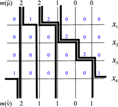
Figure 2: An example of a lattice configuration in terms of non-intersecting paths for $n=k=5$ and $\mu=(5,3,1)$, $\nu=(4,2,1)$.

3 Transfer matrix and Yang-Baxter algebras

We now introduce the row-to-row transfer matrix of the vertex model (6) as the partition function of a single lattice row and then identify it below as generating function of certain polynomials in a noncommutative alphabet.

Definition 3.1 (transfer matrix).

Given any two $n$-tuples $\boldsymbol{m}=(m_{1},\ldots,m_{n})$ and $\boldsymbol{m}^{\prime}=(m_{1}^{\prime},\ldots,m_{n}^{\prime})\in\mathbb{Z}_{\geq 0}^{n}$, the transfer matrix $Q(x_{i})$ of the $i^{\text{th}}$ row is defined via the elements

(10) $$Q(x_{i})_{m,m^{\prime}}:=\sum_{\begin{subarray}{c}allowed\,row\,\\ configurations\end{subarray}}z^{\frac{\text{\# of outer edges}}{2}}x_{i}^{\text{\# of horizontal edges}},$$

where the factor 1/2 in the power of the variable $z$ takes into account that the outer horizontal edges need to be identified, since we are on the cylinder.

As it is common in the discussion of vertex models we wish to identify the transfer matrix as an endomorphism of a vector space. For this purpose we now interpret the statistical variables at the lattice edges as labels of basis vectors in the vector space $\mathcal{M}=\mathop{\textstyle\bigoplus}_{m\in\mathbb{Z}_{\mathbb{\geq}0}}\mathbb{C}v_{m}$. Then a row configuration in the lattice, i.e. an assignment of statistical variables $\boldsymbol{m}=(m_{1},\ldots,m_{n})$ along one row of vertical edges, fixes a vector $v_{m_{1}}\otimes\cdots\otimes v_{m_{n}}\in\mathcal{M}^{\otimes n}$. Henceforth, we identify the tensor product $\mathcal{M}^{\otimes n}$ with $\mathbb{C}P^{+}$, the complex linear span of all the integral dominant weights of the affine Lie algebra $\widehat{\mathfrak{su}}(n)$, $P^{+}:=\left\{\left.\hat{\lambda}=\mathop{\textstyle\sum}_{i=1}^{n}m_{i}\hat{\omega}_{i}\right|~{}m_{i}\in\mathbb{Z}_{\geq 0}\right\},$ via the map $\boldsymbol{m}\mapsto\mathop{\textstyle\sum}_{i=1}^{n}m_{i}\hat{\omega}_{i}$. That is, we interpret the statistical variables $\boldsymbol{m}=(m_{1},\ldots,m_{n})$ in one row of our vertex model as Dynkin labels of an affine weight in $P^{+}$. For convenience we will sometimes denote this $n$-tuple $\boldsymbol{m}$ and the associated vector in $\mathcal{M}^{\otimes n}$ by the same symbol. By construction the row-to-row transfer matrix and the partition function are then related via

(11) $$Z_{\hat{\mu}}^{\hat{\nu}}(x_{1},\ldots,x_{n-1};z)=\langle\boldsymbol{m}(\hat{\nu}),Q(x_{n-1})\cdots Q(x_{1})\boldsymbol{m}(\hat{\mu})\rangle\;,$$

where we have introduced the inner product $\langle\boldsymbol{m,m}^{\prime}\rangle:=\prod_{i=1}^{n}\delta_{m_{i},m_{i}^{\prime}}$ which we assume to be antilinear in the first factor. Thus, the transfer matrix (10) can be interpreted as discrete time evolution operator which successively generates the paths on the cylindric square lattice. Note that for any pair of configurations $\boldsymbol{m},\boldsymbol{m}^{\prime}\in\mathcal{M}^{\otimes n}$ only a finite number of the terms making up the matrix element $\langle\boldsymbol{m},Q(x_{i})\boldsymbol{m}^{\prime}\rangle$ is non-zero. The operator $Q\in\mathop{\mathrm{E}nd}\mathcal{M}^{\otimes n}$ is therefore well-defined. We now reformulate the transfer matrix in terms of a set of more elementary, local operators which respectively increase and decrease a single Dynkin label $m_{i}$ only.

3.1 The local affine plactic algebra

For $i=1,\ldots,n$ define maps $\varphi_{i},\varphi_{i}^{\ast}\in\mathop{\mathrm{E}nd}(\mathcal{M}^{\otimes n})$ by setting

(12) $$\varphi_{i}^{\ast}\boldsymbol{m}=(m_{1},\ldots,m_{i}+1,\ldots,m_{n})$$

and

(13) $$\varphi_{i}\boldsymbol{m}=\left\{\begin{array}[]{cc}(m_{1},\ldots,m_{i}-1,\ldots,m_{n}),&m_{i}>0\\ 0,&\text{else}\end{array}\right.\;.$$

In addition let $N_{i}\boldsymbol{m}=m_{i}~{}\boldsymbol{m}$ for all $1\leq i\leq n$. These maps can be identified with the Chevalley generators of the $U_{q}\mathfrak{sl}(2)$ Verma module in the crystal limit; see [16]. They have first appeared in the context of the phase model; see [2] and references therein. In [15] the following statement has been proven by constructing an explicit basis for the phase algebra $\Phi$.

Proposition 3.2 (phase algebra)

The $\varphi_{i},\varphi_{i}^{\ast}$ and $N_{i}$ generate a subalgebra $\hat{\Phi}$ of $\mathop{\mathrm{E}nd}(\mathcal{M}^{\otimes n})$ which can be realized as the algebra $\Phi$ with the following generators and relations for $1\leq i,j\leq n$:

(14) $$\varphi_{i}\varphi_{j}=\varphi_{j}\varphi_{i},\quad\varphi_{i}^{\ast}\varphi_{j}^{\ast}=\varphi_{j}^{\ast}\varphi_{i}^{\ast},\quad N_{i}N_{j}=N_{j}N_{i}$$

(15) $$N_{i}\varphi_{j}-\varphi_{j}N_{i}=-\delta_{ij}\varphi_{i},\quad N_{i}\varphi_{j}^{\ast}-\varphi_{j}^{\ast}N_{i}=\delta_{ij}\varphi_{i}^{\ast},$$

(16) $$\varphi_{i}\varphi_{i}^{\ast}=1,\quad\varphi_{i}\varphi_{j}^{\ast}=\varphi_{j}^{\ast}\varphi_{i}\;\text{ if }\;i\neq j,$$

(17) $$N_{i}(1-\varphi_{i}^{\ast}\varphi_{i})=(1-\varphi_{i}^{\ast}\varphi_{i})N_{i}=0~{}.$$

Note that with respect to the scalar product introduced above we have $\langle\varphi_{i}^{\ast}\boldsymbol{m},\boldsymbol{m}^{\prime}\rangle=\langle\boldsymbol{m},\varphi_{i}\boldsymbol{m}^{\prime}\rangle\;$for any $\boldsymbol{m},\boldsymbol{m}^{\prime}\in\mathcal{M}^{\otimes n}$.

Definition 3.3 (local affine plactic algebra).

Let $\mathop{\mathrm{P}l}=\mathop{\mathrm{P}l}(\mathcal{A})$ be the free algebra generated by the elements of $\mathcal{A}=\{a_{1},a_{2},\ldots a_{n}\}$ modulo the relations

(18) $$a_{i}a_{j}-a_{j}a_{i}=0, \text{ if $|i-j|\neq 1\mod n$},$$

(19) $$a_{i+1}a_{i}^{2}=a_{i}a_{i+1}a_{i}, a_{i+1}^{2}a_{i}=a_{i+1}a_{i}a_{i+1},$$

where (19) are the plactic relations on the circle, i.e. all indices are defined modulo $n$. Denote by $\mathop{\mathrm{P}l}_{\mathop{\mathrm{f}in}}=\mathop{\mathrm{P}l}_{\mathop{\mathrm{f}in}}(\mathcal{A}^{\prime})$ the local finite plactic algebra generated from $\mathcal{A}^{\prime}=\{a_{1},a_{2},\ldots a_{n-1}\}$.

We recall the following result from [15, Prop 5.8]:

Proposition 3.4

There is a homomorphism of algebras $\mathop{\mathrm{P}l}_{\mathop{\mathrm{f}in}}\rightarrow\Phi$ such that

(20) $$a_{j}\mapsto\varphi_{j+1}^{\ast}\varphi_{j},\quad j=1,...,n-1,$$

where the representation of the phase algebra $\Phi$ given by (12) and (13) lifts to a representation of the local plactic algebra $\mathop{\mathrm{P}l}_{\mathop{\mathrm{f}in}}$. Mapping $a_{0}=a_{n}$ to $z\varphi_{1}^{\ast}\varphi_{n}$ it lifts in addition to a representation of $\mathop{\mathrm{P}l}$ on $\mathcal{M}[z]^{\otimes n}$ with $\mathcal{M}[z]=\mathbb{C}[z]\otimes_{\mathbb{C}}\mathcal{M}$ and $z$ an indeterminate. Both representations are faithful.

Remark.

The finite plactic algebra first appeared in the context of the Robinson-Schensted correspondence: given a word in a noncommutative alphabet it can be mapped onto a pair of Young tableaux, usually called $(P,Q)$, by using the bumping algorithm. $Q$ is the recording tableau encoding the sequence of bumping processes; see e.g. [6] for an explanation. Lascoux and Schützenberger showed that identifying words which only differ in their recording tableaux is equivalent to a set of identities of which (19) are special cases. The local finite plactic algebra was first considered by Fomin and Greene in [5]. We recover their case when specialising to $z=0$.

Remark.

Note that the action of the affine plactic algebra is blockdiagonal with respect to the decomposition $\mathbb{C}P^{+}=\mathop{\textstyle\bigoplus}_{k\geq 0}\mathbb{C}P_{k}^{+}$. In fact each subspace can be represented as a directed coloured graph where the elements in $P_{k}^{+}$ are the vertices and a directed edge of colour $i$ between two vertices, $\hat{\mu}\overset{i}{\longrightarrow}\hat{\lambda}$, is introduced if $\hat{\lambda}=a_{i}\hat{\mu}$. This yields the Kirillov-Reshetikhin crystal graph $\mathcal{B}_{1,k}$ of type A. Setting $z=0$ all edges related to the affine generator $a_{n}$ are removed from the graph and we obtain the $\mathfrak{su}(n)$ crystal graph of highest weight $k\omega_{1}$, where $\omega_{1}$ is the first fundamental weight.

3.2 Yang-Baxter algebras

For $r,s\in\mathbb{Z}_{\geq 0}$ arbitrary but fixed and $u$ a formal, invertible variable define $\boldsymbol{Q}(u):\mathcal{M}(u)\otimes\mathcal{M}(u)^{\otimes n}\rightarrow\mathcal{M}(u)\otimes\mathcal{M}(u)^{\otimes n}$ by setting $\boldsymbol{Q}(u)v_{r}\otimes\boldsymbol{m}:=\sum_{s\geq 0}v_{s}\otimes\boldsymbol{Q}_{s,r}(u)\boldsymbol{m}$ where

(21) $$\boldsymbol{Q}_{s,r}(u):=\sum_{\varepsilon}u^{|\varepsilon|+r}(\varphi_{1}^{\ast})^{r}a_{1}^{\varepsilon_{1}}\cdots a_{n-1}^{\varepsilon_{n-1}}\varphi_{n}^{s}$$

with the sum running over all compositions $\varepsilon=(\varepsilon_{1},\ldots,\varepsilon_{n-1})$. Despite the sums in the definition of $\boldsymbol{Q}(u)$ being infinite, only a finite number of terms survive when acting on a vector in $\mathcal{M}(u)^{\otimes n+1}$, thus the operator is well-defined. In fact, we have the following [16]:

Lemma 3.5

Let $Q$ be the transfer matrix defined in (10). Then

(22) $$Q(x_{i})=\sum_{r\geq 0}z^{r}\boldsymbol{Q}_{r,r}(x_{i})=\sum_{r\geq 0}(zx_{i})^{r}(\varphi_{1}^{\ast})^{r}\boldsymbol{Q}_{0,0}(x_{i})\varphi_{n}^{r},$$

in other words for $z=1$ the transfer matrix is the formal trace of the matrix (21).

Define another operator $\mathcal{R}(u/v):\mathcal{M}(u)\otimes\mathcal{M}(v)\rightarrow\mathcal{M}(u)\otimes\mathcal{M}(v)$ via the relation

(23) $$\mathcal{R}(u)~{}v_{a}\otimes v_{b}=\sum_{c,d\geq 0}\mathcal{R}_{c,d}^{a,b}(u)~{}v_{c}\otimes v_{d},$$

setting

(24) $$\mathcal{R}_{c,d}^{a,b}(u)=\left\{\begin{array}[]{cc}u^{a},&c=b,\;d=a\\ u^{a}(1-u),&d=a+b-c,\;b>c\\ 0,&\text{else}\end{array}\right.\;.$$

Proposition 3.6

The $\mathcal{R}$-matrix (23) and the monodromy matrix (21) obey the Yang-Baxter equation,

(25) $$\mathcal{R}_{12}(u/v)\boldsymbol{Q}_{1}(u)\boldsymbol{Q}_{2}(v)=\boldsymbol{Q}_{2}(v)\boldsymbol{Q}_{1}(u)\mathcal{R}_{12}(u/v)\;.$$

Figure 4: The (Boltzmann) weights of local vertex configuration for the auxiliary matrix $T=A+zD$. Note that in contrast to the Boltzmann weights (6) the walkers can now propagate horizontally but only one is allowed on a horizontal edge at a time.

The definition of the monodromy matrix (21) can be algebraically motivated by taking a special limit of the intertwiner of a $U_{q}(\mathfrak{sl}(2))$ Verma module; see the discussion in [16]. Replacing this Verma module with the (two-dimensional) fundamental representation one obtains in the analogous limit now a $2\times 2$ monodromy matrix, $\boldsymbol{T}\in\mathop{\mathrm{E}nd}(\mathbb{C}^{2}\otimes\mathcal{M}(u)^{\otimes n})$, where the ordering of the noncommutative alphabet is reversed($r,s=0,1$),

(26) $$\boldsymbol{T}_{r,s}(u):=\sum_{\varepsilon_{i}=0,1}u^{|\varepsilon|+s}\varphi_{n}^{s}a_{n-1}^{\varepsilon_{n-1}}\cdots a_{1}^{\varepsilon_{1}}(\varphi_{1}^{\ast})^{r}=\left(\begin{array}[]{cc}A(u)&B(u)\\ C(u)&D(u)\end{array}\right)_{r,s}\;.$$

Note that the sum now only runs over compositions $\varepsilon$ whose parts are 0 or 1. This second monodromy matrix coincides with the matrix introduced by Bogoliubov, Izergin and Kitanine in the context of the so-called phase model [2].

Proposition 3.7 ([2])

The $2\times 2$ matrix (26) with entries in $\mathop{\mathrm{E}nd}(\mathcal{M}(u)^{\otimes n})$ obeys the Yang-Baxter equation $R_{12}(u/v)\boldsymbol{T}_{1}(u)\boldsymbol{T}_{2}(v)=\boldsymbol{T}_{2}(v)\boldsymbol{T}_{1}(u)R_{12}(u/v)$ with

(27) $$R(u)=\left(\begin{array}[]{cccc}\frac{u}{u-1}&0&0&0\\ 0&0&\frac{u}{u-1}&0\\ 0&\frac{1}{u-1}&1&0\\ 0&0&0&\frac{u}{u-1}\end{array}\right)\;.$$

The matrix elements of (26) obey certain commutation relations with the matrix elements (21), which again can be encoded in yet another solution to the Yang-Baxter equation [16].

Proposition 3.8

The monodromy matrices (21) and (26) satisfy the equation,

(28) $$L_{12}^{\prime}(u/v)\boldsymbol{T}_{1}(u)\boldsymbol{Q}_{2}(v)=\boldsymbol{Q}_{2}(v)\boldsymbol{T}_{1}(u)L_{12}^{\prime}(u/v),$$

where the endomorphism $L^{\prime}\in\mathop{\mathrm{E}nd}(\mathbb{C}^{2}\otimes\mathcal{M}(u)^{\otimes n})$ is defined in terms the matrix elements

(29) $$L_{c,d}^{\prime a,b}(u)=\left\{\begin{array}[]{cc}1+u,&a,b,c,d=0\\ u^{a},&d=a+b-c,\;b\geq c,\;a,c=0,1\\ 0,&\text{else}\end{array}\right.\;.$$

Figure 5: An example of a row configuration for the auxiliary matrix $T$ for $n=6$ and $k=7$. The statistical weight is again obtained by counting the horizontal edges of paths, where outer edges are once more identified each contributing a power of $z$.

The hallmark of an exactly solvable or integrable model in statistical mechanics is that its transfer matrix commutes with itself for arbitrary values of the spectral parameter which here is identified with the variables $x_{i}$ in each lattice row. In a physical application the row variables $\{x_{1},\ldots,x_{n}\}$ would be evaluated in the interval $[0,1]^{\times n}$ such that the Boltzmann weights (6) can be interpreted as proper probabilities. The transfer matrices for any other, possibly complex values, of the $x_{i}$’s would be seen as a “symmetry” of the system. Generalising the notion of Liouville integrability in classical mechanics, such a statistical model is called integrable. One important consequence of the Yang-Baxter equations stated above is that they imply integrability of the vertex model (6).

Corollary 3.9 (Integrability)

Set $T=A+zD$ then we have, among others, the commutation relations

(30) $$[Q(u),Q(v)]=[T(u),T(v)]=[T(u),Q(v)]=0,$$

where $Q$ is the transfer matrix (10). Moreover, the following relation holds true

(31) $$\boldsymbol{Q}_{r,r}(u)B(v) = \left(1+\frac{u}{v}\right)\delta_{r,0}B(v)\boldsymbol{Q}_{0,0}(u)$$

$$+\boldsymbol{Q}_{r-1,r}(u)D(v)-\boldsymbol{Q}_{r,r+1}(u)A(v)+\boldsymbol{Q}_{r-1,r+1}(u)C(v)$$

Note in particular that the first relation in (30) entails via (11) that the partition function (7) is symmetric in the variables $x_{i}$ as claimed earlier.

3.3 Affine plactic elementary and complete symmetric polynomials

To keep this article self-contained and motivate the definition of the affine plactic polynomials below, we review some basic facts about symmetric functions; see [18] for details. Let $\{y_{1},\ldots,y_{\ell}\}$ be a set of commuting variables for some finite $\ell>0$. Recall that the ring of symmetric functions $\mathbb{C}[y_{1},\ldots,y_{\ell}]^{\mathbb{S}_{\ell}}$ is generated by either the elementary or complete symmetric functions denoted by the letters $e_{r}$ and $h_{r}$ with $r\in\mathbb{Z}_{\geq 0}$, respectively. Both sets of functions can be introduced via the following generating functions,

(32) $$\prod_{i=1}^{\ell}(1+y_{i}u) = \sum_{r\geq 0}e_{r}(y_{1},\ldots,y_{\ell})u^{r}$$

(33) $$\prod_{i=1}^{\ell}(1-y_{i}u)^{-1} = \sum_{r\geq 0}h_{r}(y_{1},\ldots,y_{\ell})u^{r},$$

respectively. Note that the first sum is finite, i.e. $e_{r}(y_{1},\ldots,y_{\ell})=0$ for $r>\ell$, while the second one is infinite. Explicitly, the elementary and complete symmetric functions are given by the expressions

(34) $$e_{r}(y_{1},\ldots,y_{\ell}) = \sum_{1\leq i_{1}<\cdots<i_{r}\leq\ell}y_{i_{1}}\cdots y_{i_{r}}\text{\quad}$$

(35) $$h_{r}(y_{1},\ldots,y_{\ell}) = \sum_{1\leq i_{1}\leq\cdots\leq i_{r}\leq\ell}y_{i_{r}}\cdots y_{i_{1}}\;.$$

From the generating functions it is immediate to deduce that the $e$’s and $h$’s satisfy recursion relations. Namely, one has the identities

(36) $$e_{r}(y_{1},\ldots,y_{\ell}) = e_{r}(y_{1},\ldots,y_{\ell-1})+y_{\ell}e_{r-1}(y_{1},\ldots,y_{\ell-1}),$$

(37) $$h_{r}(y_{1},\ldots,y_{\ell}) = h_{r}(y_{1},\ldots,y_{\ell-1})+y_{\ell}h_{r-1}(y_{1},\ldots,y_{\ell})\;.$$

As mentioned above one has $\mathbb{C}[y_{1},\ldots,y_{\ell}]^{\mathbb{S}_{\ell}}\cong\mathbb{C}[e_{1},\ldots,e_{\ell}]\cong\mathbb{C}[h_{1},\ldots,h_{\ell}]$ and, thus, both sets of functions must be polynomials of each other. In fact, multiplying both generating functions (with $u$ replaced by $-u$ in the first one) yields the equations $\sum_{r=a+b}(-1)^{a}e_{a}h_{b}=0$ for all $r\geq 0$ which can be solved either for the $e$’s or the $h$’s to yield the well-known Jacobi-Trudi formulae

(38) $$h_{r}(y_{1},\ldots,y_{\ell}) = \det(e_{1-i+j}(y_{1},\ldots,y_{\ell}))_{1\leq i,j\leq r},$$

(39) $$e_{r}(y_{1},\ldots,y_{\ell}) = \det(h_{1-i+j}(y_{1},\ldots,y_{\ell}))_{1\leq i,j\leq r}\;.$$

We will now generalise these functions by replacing the commuting variables $\{y_{1},\ldots,$ $y_{\ell}\}$ with the noncommutative variables $\{a_{1},\ldots,a_{n}\}$, i.e. the generators of the affine plactic algebra. We wish to identify the auxiliary matrix $T$ defined in Corollary 3.9, the trace of (26), and the transfer matrix $Q$ defined either through (10) or (22) as noncommutative analogues of the generating functions (32) and (33), respectively. When trying to generalise (34) and (35) to a noncommutative alphabet one needs to specify an ordering of the variables. The auxiliary and transfer matrix prescribe such an ordering of the noncommutative variables $\{a_{i}\}$ which turns out to be consistent and has the additional desirable property that the resulting affine plactic elementary and complete symmetric polynomials form a commutative subalgebra due to the integrability condition (30). Because this ordering is cyclic, it is easier to split the affine generator $a_{n}$ into its constituents $z,\varphi_{1}^{\ast}$ and $\varphi_{n}$, compare with Proposition 3.4, and write the variables in descending or ascending order as we have already done in (26) and (21).

Proposition 3.10 (generating functions)

The transfer matrix (10) can be interpreted as the generating function

(40) $$Q(x_{i})=\sum_{r\geq 0}z^{r}\boldsymbol{Q}_{r,r}(x_{i})=\sum_{r\geq 0}x_{i}^{r}h_{r}(\mathcal{A})$$

of the affine plactic complete symmetric polynomials

(41) $$h_{r}(\mathcal{A}):=\sum_{\varepsilon\vdash r}z^{\varepsilon_{0}}(\varphi_{1}^{\ast})^{\varepsilon_{0}}a_{1}^{\varepsilon_{1}}\cdots a_{n-1}^{\varepsilon_{n-1}}\varphi_{n}^{\varepsilon_{0}}\;.$$

The auxiliary matrix defined in Corollary 3.9,

(42) $$T(x_{i})=A(x_{i})+zD(x_{i})=\sum_{r\geq 0}x_{i}^{r}e_{r}(\mathcal{A}),$$

on the other hand, yields the generating function of the affine plactic elementary symmetric polynomials,

(43) $$e_{r}(\mathcal{A}):=\sum_{\begin{subarray}{c}\varepsilon\vdash r\\ \varepsilon_{i}=0,1\end{subarray}}z^{\varepsilon_{n}}\varphi_{n}^{\varepsilon_{n}}a_{n-1}^{\varepsilon_{n-1}}\cdots a_{1}^{\varepsilon_{1}}(\varphi_{1}^{\ast})^{\varepsilon_{n}}$$

3.4 Combinatorial description of the Yang-Baxter algebra

Note that when setting the quasi-periodicity parameter $z$ to zero, i.e. enforcing open boundary conditions, one obtains the finite plactic polynomials of [5]. For instance, we have that the matrix element $A$ in (26) is the generating function of the finite plactic elementary polynomials,

(44) $$z=0:\qquad A(u)=(1+a_{n-1}u)\cdots(1+a_{1}u)=\sum_{r\geq 0}u^{r}e_{r}(\mathcal{A}^{\prime})\;.$$

Lemma 3.11

The action of the operator $e_{r}(\mathcal{A}^{\prime})=e_{r}(a_{1},\ldots,a_{n-1})$ on a partition $\mu\in\mathcal{P}_{\leq n-1,k}$ produces a sum over all partitions $\lambda$ in the $n\times k$ bounding box such that the skew diagram $\lambda/\mu$ is a vertical strip of length $r$ and $\lambda_{1}=\mu_{1}$,

(45) $$e_{r}(\mathcal{A}^{\prime})\mu=\sum_{\lambda\in\mathcal{P}_{\leq n,k},\;\lambda/\mu=(1^{r})}\delta_{\lambda_{1},\mu_{1}}\lambda^{\prime}\;.$$

Here $\lambda^{\prime}\in\mathcal{P}_{\leq n-1,k}$ is the partition obtained from $\lambda$ by deleting all columns of height $n$.

Proof.

Using the graphical depiction of the Boltzamnn weights in Figure 4 it follows that for $z=0$ only row configurations are allowed which do not have an occupied outer horizontal edge. Hence, $m_{1}(\mu)\geq m_{1}(\nu)$ which entails that we must have $\mu_{1}=\nu_{1}$ according to (2). Moreover, we can deduce from the Boltzmann weights that $m_{i}(\nu)-m_{i}(\mu)=0$ or 1 for $i>1$, hence $\lambda/\mu$ must be a horizontal $r$-strip.    

In order to describe the action of the remaining matrix elements in (26) note that in terms of partitions the map $\varphi_{1}^{\ast}$ adds a column of height one and increases the width of the bounding box, the level $k$, by one. The map $\varphi_{n}$ simply decreases the width of the bounding box if $\lambda_{1}<k$, otherwise it sends $\lambda$ to zero. Thus, the following formulae

(46) $$B(u)=u~{}A(u)\varphi_{1}^{\ast},\qquad C(u)=\varphi_{n}A(u),\qquad D(u)=u\varphi_{n}A(u)\varphi_{1}^{\ast}~{},$$

which can be easily checked from (26), allow one to perform computations with the Yang-Baxter algebra purely in terms of Young diagrams and their bounding boxes.

Example 3.12.

Let $n=5$ and choose $\mu=(2,2,1,0)$ with $\boldsymbol{m}=(0,1,1,0,1)$, that is $k=3$. Then we have for $r=3$ only a single term,

$$\Yvcentermath 1e_{3}(\mathcal{A}^{\prime})~{}\yng(2,2,1)=\Yvcentermath 1\yng(2,2,2,1,1)\equiv\Yvcentermath 1\yng(1,1,1)\;.$$

In contrast the action of the affine plactic polynomial yields the sum

$$\Yvcentermath 1e_{3}(\mathcal{A})~{}\yng(2,2,1)=\Yvcentermath 1\yng(1,1,1)~{}+z~{}\yng(3,3,2)~{}+z~{}\yng(3,3,1,1)~{}+z~{}\yng(3,2,2,1)~{}+z~{}\yng(2,1)\;.$$

By converting each partition in the above sum to the corresponding compositions one verifies that each of the last four terms on the right hand side is generated by a monomial in $\mathcal{A}$ which contains the affine generator $a_{n}$. For instance, for the second term one finds

$$\Yvcentermath 1z~{}\underset{\boldsymbol{m}=(0,1,2,0,0)}{\yng(3,3,2)}=\Yvcentermath 1z\varphi_{5}a_{2}a_{1}\varphi_{1}^{\ast}~{}\underset{\boldsymbol{m}=(0,1,1,0,1)}{\yng(2,2,1)}=\Yvcentermath 1a_{2}a_{1}a_{5}~{}\yng(2,2,1)\;,$$

where we have used (16) to rewrite the respective term in $e_{3}(\mathcal{A})$ as word in the affine plactic generators. This is always possible for $r<n$.

In light of (44) and the last example the definition of the auxiliary matrix (42) can be seen as the noncommutative analogue of (36), since after expanding with respect to the variable $u$ one arrives at the identity

(47) $$e_{r}(\mathcal{A})=e_{r}(\mathcal{A}^{\prime})+z\varphi_{n}e_{r-1}(\mathcal{A}^{\prime})\varphi_{1}^{\ast}\;.$$

Cylic ordering. As already alluded to in the last example comparison with the commutative case (36) is made easier by realising that for $r<n$ the terms in the second summand can always be rearranged in cyclic order. To expose the general structure more clearly consider another example provided by the row configuration depicted in Figure 5 for $n=6$ and $k=7$. The latter corresponds via (43) to the monomial

$$z\varphi_{6}a_{5}a_{4}a_{2}a_{1}\varphi_{1}^{\ast}=za_{2}a_{1}\varphi_{6}a_{5}a_{4}\varphi_{1}^{\ast}=a_{2}a_{1}a_{6}a_{5}a_{4},$$

where we have used once more (16). The general case is now clear: monomials in the $a_{i}$ which do neither contain $a_{1}$ or $a_{n}$, or only one of these generators, are always written in descending order from left to right. If both, $a_{1}$ and $a_{n},$ occur in the same monomial write the maximal string of form $a_{l}a_{l-1}\cdots a_{2}a_{1}$ to the left of the remaining letters which should also be in descending order starting with $a_{n}$ (although the indices might now “jump”by more than one). It follows from the definition (43) that for $r=n$ we have $e_{n}(\mathcal{A})=z\cdot 1$.

We now specialise to the finite plactic complete symmetric polynomials,

(48) $$z=0:\qquad Q(u)=\boldsymbol{Q}_{0,0}(u)=\sum_{r\geq 0}u^{r}h_{r}(\mathcal{A}^{\prime})\;.$$

From the definition (41) one easily computes the noncommutative analogue of the recursion relation (37),

(49) $$h_{r}(\mathcal{A})=h_{r}(\mathcal{A}^{\prime})+z\varphi_{1}^{\ast}h_{r-1}(\mathcal{A})\varphi_{n}\;.$$

Lemma 3.13

Let $r\leq k$ and $\mu\in\mathcal{P}_{\leq n-1,k}$ then

(50) $$h_{r}(\mathcal{A}^{\prime})\mu=\sum_{\lambda\in\mathcal{P}_{\leq n,k},\;\lambda/\mu=(r)}\delta_{\lambda_{1},\mu_{1}}\lambda^{\prime}\;.$$

For $r>k$ we have $h_{r}(\mathcal{A}^{\prime})|_{\mathbb{C}P_{k}^{+}}=0$.

Proof.

The assertion follows from a similar line of argument as before, but this time one uses the Boltzmann weights depicted in Figure 1. Since $z=0$ row configurations with outer edges are prohibited, whence $m_{1}(\mu)\geq m_{1}(\nu)$. In contrast to the previous case (45) a friendly walker now cannot propagate horizontally, however several are allowed at the same time on the horizontal edges. Thus, we obtain a horizontal instead of a vertical strip. The last identity is also clear from the graphical depiction of allowed row configurations: the number of occupied horizontal edges cannot exceed the number of incoming walkers.    

Note that the affine plactic complete symmetric polynomials can only be rewritten in (reverse) cyclic order for $r<n$ using the same commutation relations of the phase algebra as before. For $r>n$ the cyclic ordering ceases to be well-defined and one has to resort to (41).

Finally, we generalise the last identities from the commutative case, the Jacobi-Trudi formulae (38) and (39), which are subject of the next proposition [16].

Proposition 3.14 (operator functional equation)

The generating functions (40) and (42) satisfy the operator functional relation,

(51) $$T(-u)Q(u)=1+z(-1)^{n}\sum_{k\geq 0}u^{k+n}h_{k}(\mathcal{A})\pi_{k}\;,$$

where $\pi_{k}:\mathbb{C}P^{+}\rightarrow\mathbb{C}P_{k}^{+}$ is the projector onto the subspace spanned by the weights at level $k$. In particular, for $r<n+k$ the familiar determinant relations from the commutative case also hold for the noncommutative elementary and complete symmetric polynomials,

(52) $$h_{r}(\mathcal{A})=\det(e_{1-i+j}(\mathcal{A}))_{1\leq i,j\leq r},\qquad e_{r}(\mathcal{A})=\det(h_{1-i+j}(\mathcal{A}))_{1\leq i,j\leq r}\;,$$

where the determinants are well defined due to (30).

Figure 6: The two possible vacuum row configurations of the auxiliary matrix $T$. Note that the transfer matrix $Q$ only allows for the left one.

Figure 7: Depicted is the row configuration resulting from the successive action of the transfer matrix $Q$ and the operator $D$ on a state of level $k=1$ and which is responsible for the additional term on the right hand side of the functional equation (51).

Setting once more $z=0$ we recover the relation expected from the commutative case. The additional terms have their origin in the quasi-periodic boundary conditions and we explain their origin on an example which will elucidate the general formula.

Example 3.15.

Set $n>2$ and consider first the case of level $k=0$. There is only one state, the “pseudo-vacuum” $\hat{\Omega}=(0,0,\ldots,0)$, and trivially we have $Q(u)\hat{\Omega}=\hat{\Omega}$. Acting with $T(-u)$ on $\hat{\Omega}$ we obtain two contributions shown in Figure 6. Thus, the additional term in (51) with $h_{0}(\mathcal{A})=1$ is due to a “vacuum mode”, a path which winds around the cylinder.

Let us now set $k=1$ and consider the state $\hat{\omega}_{i}=(0,\ldots,0,\underset{i}{1},0,\ldots 0)$ with $i<n$. Then $Q(u)\hat{\omega}_{i}=\hat{\omega}_{i}+u\hat{\omega}_{i+1}$ as can be deduced graphically from (10). In order to understand the origin of the additional term in (51) which includes the factor $z$, it suffices to look at the contribution from the $D$ operator, since $T=A+zD$ and $A,D$ do not contain $z$. The action of $D$ can be easily computed using Figure 4 and remembering that only row configurations contribute where the outer edges are occupied. One finds that all row configurations cancel except for one term which is depicted in Figure 7: again the additional term in (51) corresponds to a diagram where one path winds around the cylinder.

3.5 Quantum Hamiltonian and particle picture

So far we discussed a statistical mechanics model whose transfer matrix can be identified with the generating function of the affine plactic complete symmetric polynomials. Similarly, we can link the generating function of the affine plactic elementary symmetric polynomials, the auxiliary matrix $T$, to a physical model in quantum mechancis. Interpret the Dynkin labels $m_{i}$ as occupation numbers of a site $i$ of a circular lattice - the Dynkin diagram of $\widehat{\mathfrak{su}}(n)$ in Figure 8 - and the maps (12) and (13) as particle creation and annihilation operators, respectively. Introducing the quantum Hamiltonian

(53) $$H=-\frac{e_{1}(\mathcal{A})+e_{n-1}(\mathcal{A})}{2}=-\frac{1}{2}\sum_{j=1}^{n}(\varphi_{j+1}^{\ast}\varphi_{j}+z\varphi_{j}^{\ast}\varphi_{j+1})$$

with $\varphi_{n+1}=z^{-1}\varphi_{1},\;\varphi_{n+1}^{\ast}=z\varphi_{1}^{\ast}$, as well as the conserved charges $H_{r}^{\pm}=-(e_{r}(\mathcal{A})\pm e_{n-r}(\mathcal{A}))/2$ which because of (30) are in involution, $[H,H_{r}^{\pm}]=[H_{r}^{\pm},H_{r^{\prime}}^{\pm}]=0$, yields an alternative physical interpretation of the combinatorial structures described here. This quantum system is known as phase model, see [2] and references therein.

Figure 8: The fusion ring can be interpreted as a discrete model in quantum mechanics. Each Dynkin label $m_{i}$ specifies a number of particles sitting at the $i^{\text{th}}$ node of the Dynkin diagram. Application of the generator $a_{i}$ of the affine plactic algebra, shifts one particle from site $i$ to site $i+1$, as indicated in the picture for $i=1$.

4 Bethe ansatz equations and the fusion potential

Within the framework of exactly solvable models the next step is to construct the eigenvectors of the transfer matrix $Q$. Instead it is simpler to consider the eigenvalue problem of the auxiliary matrix $T$, since it follows from the functional relation (51) and the determinant formulae (52) that the eigenvectors of $Q$ coincide with the eigenvectors of $T$. The advantage of this approach is that the eigenvectors of $T$ can be computed via the algebraic Bethe ansatz or quantum inverse scattering method (see e.g. [3] for a text book and references therein) using the commutation relations of the $A,B,C,D$ algebra in (26), which are drastically simpler than the commutation relations of the algebra generated by the matrix elements (21). Starting point is a particular assumption on the algebraic form of the eigenvectors: define an (off-shell) Bethe vector at level $k>0$ to be

(54) $$b(x_{1},\ldots,x_{k}):=B(x_{1}^{-1})\cdots B(x_{k}^{-1})\hat{\Omega},$$

where $\hat{\Omega}$ is again the unique vector corresponding to the composition $(0,0,\ldots,0)$. The requirement that (54) is an eigenvector of $T$ leads via the commutation relations of the Yang-Baxter algebra contained in (27) and a standard computation - which we omit - to the Bethe ansatz equations [2] [15]

(55) $$x_{1}^{n+k}=\cdots=x_{k}^{n+k}=z(-1)^{k-1}\prod_{i=1}^{k}x_{i}\;.$$

We now discuss how the Bethe ansatz equations lead to a combinatorial computation of fusion coefficients. We wish to emphasize that this is possible without solving (55) first. For this reason we postpone the discussion of their solutions to the next section, however, we already mention that in order to solve them one needs to assume that $z^{\pm 1/n}$ exist.

The Bethe ansatz equations are $k$ polynomial equations and, thus, describe an affine variety $\mathbb{V}_{n,k}^{\prime}\subset\mathbb{C}[z^{\pm\frac{1}{n}}]^{k}$. Recall that given a field $\mathbb{K}$ an affine variety is usually defined in terms of a set of polynomials $f_{1},\ldots,f_{k}\in\mathbb{K}[x_{1},\ldots,x_{k}]$ by setting $\mathbb{V}(f_{1},\ldots,f_{k}):=\left\{v\in\mathbb{K}^{k}:f_{i}(v_{1},\ldots,v_{k})=0,\text{ }i=1,\ldots,k\right\}$. Note that due to the commutation relations $B(x)B(y)=B(y)B(x),$ which follow from the Yang-Baxter equation (27), we can identify solutions of (55) under permutations $(x_{1},\ldots,x_{k})\sim(x_{w_{1}},\ldots,x_{w_{k}})$ for all $w\in\mathbb{S}_{k},$ since they give rise to the same eigenvector (54). Denote by $\mathbb{V}_{n,k}$ the variety obtained under this identification, then we can think of $\mathbb{V}_{n,k}$ as being defined by $k$ elements in the ring of symmetric polynomials $\mathbb{C}[z^{\pm\frac{1}{n}}]^{k}[x_{1},\ldots,x_{k}]^{\mathbb{S}_{k}}\cong\mathbb{C}[z^{\pm\frac{1}{n}}]^{k}[e_{1},\ldots,e_{k}]$, where the $e_{i}$’s are the elementary symmetric functions.

Lemma 4.1

Let $h_{r}=\det(e_{1-i+j})_{1\leq i,j\leq r}$, the complete symmetric functions, then the affine variety $\mathbb{V}_{n,k}$ defined by the Bethe ansatz equations (up to permutations of the solutions) is given by

(56) $$\mathbb{V}_{n,k}=\mathbb{V}(h_{n}-z,h_{n+1},\ldots,h_{n+k-1})\;.$$

The proof of this statement can be found in [15, Lemma 6.3] and simply uses the recursive relation (37) for complete symmetric polynomials. Next we assign to the solutions of the Bethe ansatz equations (55) an ideal in the ring of symmetric functions. Recall the definition of the nullstellen or vanishing ideal of an affine variety $\mathbb{V}$, $\mathcal{I}(\mathbb{V}):=\{f\in\mathbb{C}(z)[e_{1},\ldots,e_{k}]:f(v)=0,\;v\in\mathbb{V}\}$. Then we have the following statement [15, Proof of Theorem 6.20]:

Proposition 4.2

Let $\mathcal{I}(\mathbb{V}_{n,k})$ be the nullstellen ideal of the Bethe ansatz variety (56), then

(57) $$\langle h_{n}-z,h_{n+1},\ldots,h_{n+k-1}\rangle=\mathcal{I}(\mathbb{V}_{n,k})\;.$$

This proposition is proved via Hilbert’s Nullstellensatz which asserts that given an ideal $I$ in a polynomial ring one has $\mathcal{I}(\mathbb{V}(I))=\sqrt{I},$ where $\sqrt{I}=\{f:f^{m}\in I$ for some $m\in\mathbb{Z}_{>0}\}$ is the radical of $I$. In the present case where $I=\langle h_{n}-1,h_{n+1},\ldots,h_{n+k-1}\rangle$ one shows that $I=\sqrt{I}$ and thus the assertion follows from the previous lemma.

Remark.

For $z=1$ the ideal (57) can be encoded into a fusion potential $V^{\prime}_{k+n}=p_{k+n}/(k+n)+(-1)^{k}e_{k}$ with $p_{k+n}=\sum_{i=1}^{k}x_{i}^{n+k}$, the $(k+n)^{\text{th}}$ power sum, noting that

$$\frac{1}{k+n}\frac{\partial p_{k+n}}{\partial e_{r}}=(-1)^{r-1}h_{k+n-r}=0,\qquad r=1,2,\ldots,k\;.$$

This is very similar to the fusion potential introduced by Gepner. The difference lies in the constraints imposed on the variables: Gepner’s fusion potential [7, Equation (2.31)]

(58) $$V_{n+k}=\frac{1}{k+n}\sum_{i=1}^{n}y_{i}^{n+k},$$

is defined in terms of $n$ variables $\{y_{1},\ldots,y_{n}\}$ subject to the constraints $e_{n}(y)=y_{1}\cdots y_{n}=1$ and

(59) $$\frac{\partial V_{n+k}}{\partial e_{i}}=(-1)^{i+1}h_{n+k-i}=0,\quad i=1,\ldots,n-1\;.$$

These constraints can be shown to be equivalent with the following set of equations,

(60) $$y_{1}^{n+k}=\cdots=y_{n}^{n+k}=h_{k+n}(y_{1},\ldots,y_{n})=(-1)^{n-1}h_{k}(y_{1},\ldots,y_{n}),$$

which look very similar to the Bethe ansatz equations (55). However, the corresponding construction of the Bethe vector in terms of a Yang-Baxter algebra is currently missing.

The importance of the ideal (57) derived form the Bethe ansatz equations lies in the fact that it yields a presentation of the Verlinde or fusion algebra in the ring of symmetric functions [15, Theorem 6.20].

Theorem 4.3 (Korff-Stroppel)

Set $z=1$. Then the map $P_{k}^{+}\ni\hat{\lambda}\mapsto s_{\lambda^{t}}+\mathcal{I}(\mathbb{V}_{n,k}),$ where $\mathcal{I}(\mathbb{V}_{n,k})$ is the ideal in (57) provides an algebra isomorphism,

(61) $$\mathcal{F}_{n,k}\otimes_{\mathbb{Z}}\mathbb{C}\cong\mathbb{C}[e_{1},\ldots,e_{k}]/\mathcal{I}(\mathbb{V}_{n,k})\;.$$

In contrast Gepner’s fusion potential is equivalent to a different presentation; c.f. [10, p247, result (4)] and [7, Equation (2.36)].

Theorem 4.4 (Gepner, Goodman-Wenzl)

The map $P_{k}^{+}\ni\hat{\lambda}\mapsto s_{\lambda}+I_{n,k},$ where $I_{n,k}=\langle e_{n}-1,h_{k+1},\ldots,h_{n+k-1}\rangle$ is the ideal resulting from (59) also provides an isomorphism,

(62) $$\mathcal{F}_{n,k}\otimes_{\mathbb{Z}}\mathbb{C}\cong\mathbb{C}[e_{1},\ldots,e_{n}]/I_{n,k}\;.$$

Proof.

For the sake of completeness we briefly outline a proof of (62) by showing that the ideal (59) following from Gepner’s fusion potential is identical with the ideal used by Goodman and Wenzl in [10] (with the extra condition $e_{n}=1$) who proved that the fusion ring is isomorphic to a certain representation of the Hecke algebra at a primitive $(n+k)^{\text{th}}$ root of unity.

Let $J_{n,k}$ be the ideal generated from $e_{n}-1$ and the Schur polynomials of the form $s_{(\lambda_{1},\lambda_{2},\ldots,\lambda_{n})}$ with $\lambda_{1}-\lambda_{n}=k+1$; c.f. [10, p247, result (4)]. Both ideals can be shown to be radical along similar lines as it is discussed for (57) in [15, Proof of Theorem 6.20, Claim 1]. Hence, employing the Nullstellensatz twice, $\mathcal{I}(\mathbb{V}(I_{n,k}))=I_{n,k}$ and $\mathcal{I}(\mathbb{V}(J_{n,k}))=J_{n,k}$, it suffices to prove the two inclusions $J_{n,k}\subseteq\mathcal{I}(\mathbb{V}(I_{n,k}))$ and $I_{n,k}\subseteq\mathcal{I}(\mathbb{V}(J_{n,k}))$. For this purpose we recall the definition of hook Schur polynomials [18, Chapter I, Section 3, Example 9]

(63) $$s_{(a|b)}:=s_{(a+1,1^{b})}=h_{a+1}e_{b}-h_{a+2}e_{b-1}+\cdots+(-1)^{b}h_{a+b+1}\;.$$

Using the Frobenius notation $\lambda=(\alpha_{1},\ldots,\alpha_{r}|\beta_{1},\ldots,\beta_{r})$ for a partition $\lambda$, where $\alpha_{i}$ and $\beta_{i}$ are the lengths of the horizontal and vertical part of a hook centered at the $i^{\text{th}}$ box in the diagonal of $\lambda$, one has

(64) $$s_{\lambda}=\left|\begin{array}[]{cccc}s_{(\alpha_{1}|\beta_{1})}&s_{(\alpha_{1}|\beta_{2})}&\cdots&s_{(\alpha_{1}|\beta_{r})}\\ s_{(\alpha_{2}|\beta_{1})}&\ddots&&s_{(\alpha_{2}|\beta_{r})}\\ \vdots&&\ddots&\vdots\\ s_{(\alpha_{r}|\beta_{1})}&s_{(\alpha_{r}|\beta_{2})}&\cdots&s_{(\alpha_{r}|\beta_{r})}\end{array}\right|$$

We first show that $J\subseteq\mathcal{I}(\mathbb{V}(I_{n,k}))=I_{n,k}.$ Exploiting $e_{n}=1$ and the Pieri rule $e_{n}s_{(\lambda_{1},\lambda_{2},\ldots,\lambda_{n})}=s_{(\lambda_{1}+1,\lambda_{2}+1,\ldots,\lambda_{n}+1)}$ we can restrict ourselves to Schur polynomials of the form $s_{(k+1,\lambda_{2},\ldots,\lambda_{n-1},0)}$. From the definition of $I_{n,k}$ it then follows that

$$s_{(k|b)}=h_{k+1}e_{b}-h_{k+2}e_{b+1}+\cdots+(-1)^{b}h_{k+b+1}=0$$

for all $b=0,1,2,\ldots,n-2$ and, thus, we can conclude with the help of (64) that $s_{(k+1,\lambda_{2},\ldots,\lambda_{n-1},0)}=0$ for all $k+1\geq\lambda_{2}\geq\cdots\geq\lambda_{n-1}$ as required.

The converse inclusion $I_{n,k}\subset\mathcal{I}(\mathbb{V}(J_{n,k}))$ is easily derived along similar lines:

$$0 = s_{(k|0)}=s_{(k+1,0,\ldots,0)}=h_{k+1},$$

$$0 = s_{(k|1)}=h_{k+1}e_{1}-h_{k+2}=-h_{k+2},$$

$$\vdots$$

$$0 = s_{(k|n-2)}=h_{k+1}e_{n-2}-\cdots+(-1)^{n-2}h_{k+n-1}=(-1)^{n-2}h_{k+n-1}\;.$$

This shows that the ideal of Goodman and Wenzel coincides with the ideal of Gepner and using [10, p247, result (4)] we arrive at (62).    

Remark.

The two isomorphisms (61) and (62) lead to different expressions for the fusion coefficients in terms of Littlewood-Richardson coefficients. We will discuss the case (61) below. Goodman and Wenzl used their presentation (62) to derive the Kac-Walton formula [13] [20] (compare with [10, p247, result (6)]),

(65) $$\mathcal{N}_{\hat{\lambda}\hat{\mu}}^{(k)\hat{\nu}}=\sum_{w\in\hat{W}}\varepsilon(w)c_{\lambda\mu}^{(w\cdot\hat{\nu})^{\prime}},$$

where $\hat{W}$ denotes the affine Weyl group, $\varepsilon(w)$ the signature of $w$, $w\cdot\hat{\nu}=w(\hat{\nu}+\hat{\rho})-\hat{\rho}$ is the shifted Weyl group action with $\hat{\rho}=\sum_{i}\hat{\omega}_{i}$ being the affine Weyl vector and $(w\cdot\hat{\nu})^{\prime}$ is the partition obtained under the bijection (2).

Example 4.5.

Set $n=3$ and $k=4$ and consider the affine weights $\hat{\lambda}=\hat{\omega}_{0}+2\hat{\omega}_{1}+\hat{\omega}_{2}$, $\hat{\mu}=\hat{\omega}_{0}+\hat{\omega}_{1}+2\hat{\omega}_{2}$ in $P_{k}^{+}$. The corresponding partitions under (2) are $\lambda=(3,1)$ and $\mu=(3,2)$. Employing the Littlewood-Richardson rule (see e.g. [6]) yields the partitions

(66) $$\rho=(6,3,0),(6,2,1),(5,4,0),(5,3,1),(5,3,1),(5,2,2),(4,4,1),\\ (4,3,2),(4,3,2),(3,3,3),(5,2,1,1),(4,3,1,1),(4,2,2,1),(3,3,2,1)\;.$$

Discarding all partitions of length $>$ $n$ and removing all $n$-columns from the partitions $\nu$ we obtain the following $\mathfrak{su}(n)$ tensor product decomposition

$$\lambda\otimes\mu=(6,3)\oplus(5,1)\oplus(5,4)\oplus 2(4,2)\oplus(3,0)\oplus(3,3)\oplus 2(2,1)\oplus(0,0)\;.$$

Here we have identified highest weight modules with the corresponding partitions. We wish to consider the fusion coefficient of the affine weight $\hat{\nu}=2\hat{\omega}_{1}+2\hat{\omega}_{2}$ with partition $\nu=(4,2)$. From (65) we find

(67) $$\mathcal{N}_{\hat{\lambda}\hat{\mu}}^{(k)\hat{\nu}}=c_{\lambda\mu}^{(4,2)}-c_{\lambda\mu}^{(6,3)}=2-1=1,$$

since $s_{0}\cdot\widehat{(6,3)}=s_{0}\cdot(-2\hat{\omega}_{0}+3\hat{\omega}_{1}+3\hat{\omega}_{2})=\hat{\nu}$ with $s_{0}$ denoting the affine Weyl reflection. In fact, the entire fusion product expansion is computed to

(68) $$\Yvcentermath 1\yng(3,1)~{}\ast~{}\yng(3,2)=\\ \Yvcentermath 1\yng(4,2)+~{}\yng(3)+~{}\yng(3,3)+2~{}\yng(2,1)+\emptyset\;.$$

4.1 Algorithm to compute fusion coefficients

Based on the presentation (61) derived from the Bethe ansatz equations we now formulate an alternative algorithm how to compute fusion coefficients in terms of Littlewood-Richardson numbers.

1. Compute the expansion $s_{\lambda^{t}}s_{\mu^{t}}=\sum_{\rho^{t}}c_{\lambda\mu}^{\rho}s_{\rho^{t}}$ via the Littlewood-Richardson rule ; note that $c_{\lambda\mu}^{\rho}=c_{\lambda^{t}\mu^{t}}^{\rho^{t}}$ [6]. Discard all terms for which the partition $\rho^{t}$ has length $>$ $k$.

2. For each of the remaining terms with $\rho_{1}^{t}\geq n$ make the replacement $s_{\rho^{t}}=s_{(\rho_{2}^{t},\ldots,\rho_{k}^{t},\rho_{1}^{t}-n)}$. Whenever $(\rho_{2}^{t},\ldots,\rho_{k}^{t},\rho_{1}^{t}-n)$ is not a partition use the straightening rules [18]

   $$s_{(\ldots,a,b,\ldots)}=-s_{(\ldots,b-1,a+1,\ldots)}\quad\text{and}\quad s_{(\ldots,a,a+1,\ldots)}=0$$

   for Schur polynomials to rewrite $s_{(\rho_{2}^{t},\ldots,\rho_{k}^{t},\rho_{1}^{t}-n)}$ as $s_{\nu^{t}}$ with $\nu^{t}$ a partition.

3. Collecting terms for each $\nu$ one obtains the fusion coefficient $\mathcal{N}_{\hat{\lambda}\hat{\mu}}^{(k)\hat{\nu}}$.

Example 4.6.

As in example (4.5) set $n=3,\,k=4$ and consider the partitions $\lambda=(3,1,0)$ and $\mu=(3,2,0).$ After taking the transpose partitions in (66) we discard $\rho^{t}=(2,2,2,1,1,1)$, $(3,2,1,1,1,1)$, $(2,2,2,2,1)$, $(3,2,2,1,1)$, $(3,3,1,1,1)$ and $(4,2,1,1,1)$ as they have length $>$ $k=4$. We are left with three partitions $\rho^{t}$ for which $\rho_{1}^{t}>n$, namely $(4,2,2,1)$, $(4,3,1,1)$, $(4,3,2,0)$. Employing the above algorithm we calculate

$$s_{(4,2,2,1)}=s_{(2,2,1,1)},\quad s_{(4,3,1,1)}=s_{(3,1,1,1)},\quad s_{(4,3,2,0)}=s_{(3,2,0,1)}=0\;.$$

Removing all rows of length $n=3$ and collecting terms, one arrives after taking the transpose again at the expansion (68), however, the expression for the fusion coefficients in terms of Littlewood-Richardson numbers are different. For instance, the coefficient of $\nu=(4,2,0)$ is according to the Kac-Walton formula the difference of two Littlewood-Richardson coefficients, see (67). In contrast, here we find that

$$\mathcal{N}_{(3,1,0)(3,2,0)}^{(k)(4,2,0)}=c_{(3,1,0,0),(3,2,0,0)}^{(4,3,1,1)}=1$$

Thus, the Bethe ansatz equations (55) provide an alternative algorithm to compute fusion coefficients.

Proof of the algorithm.

Consider the ring of symmetric functions $\mathbb{C}[x_{1},x_{2},\ldots,x_{k}]^{\mathbb{S}_{k}}$, then $s_{\lambda}=0$ unless $\ell(\lambda)\leq k$. This justifies Step 1 of the algorithm. To deduce Step 2, assume we are given a partition $\lambda$ with $\ell(\lambda)\leq k$ and $\lambda_{1}>n$. Then we rewrite the Schur function as [18]

$$s_{\lambda}(x_{1},x_{2},\ldots,x_{k})=\sum_{w\in\mathbb{S}_{k}}w\cdot\left(x_{1}^{\lambda_{1}}\cdots x_{k}^{\lambda_{k}}\theta(x)\right),\quad\theta(x):=\prod_{1\leq i<j\leq k}\frac{1}{1-x_{j}/x_{i}}\;.$$

Observing that the equations (55) for $x_{1}$ are equivalent to

$$x_{1}^{n}\prod_{j>1}\frac{x_{1}}{x_{1}-x_{j}}=z\prod_{j>1}\frac{x_{j}}{x_{j}-x_{1}}$$

one derives the identity

$$x_{1}^{\lambda_{1}}\cdots x_{k}^{\lambda_{k}}\theta(x)=z~{}w_{0}\cdot(x_{1}^{\lambda_{2}}x_{2}^{\lambda_{3}}\cdots x_{k}^{\lambda_{1}-n}\theta(x)),$$

where $w_{0}=\sigma_{k-1}\cdots\sigma_{2}\sigma_{1}$ and $\sigma_{i}$ is the transposition which permutes $x_{i}$ and $x_{i+1}$. Insertion of this identity into the above expression for the Schur function proves that $s_{\lambda}=s_{(\lambda_{2},\lambda_{3},\ldots,\lambda_{k},\lambda_{1}-n)}+\mathcal{I}(\mathbb{V}_{n,k})$. Step 3 then follows from (61).    

5 Bethe vectors as idempotents

We now solve the Bethe ansatz equations (55) explicitly, which is possible due to their simple form, and describe the variety $\mathbb{V}_{n,k}$ which consists of a discrete set of points in $\mathbb{C}[z^{1/n}]^{k}$. For each partition $\sigma$ in $\mathcal{P}_{\leq n-1,k}$ define the following tuple of elements in $\mathbb{C}[z^{\pm 1/n}],$

(69) $$\mathcal{P}_{\leq n-1,k}\ni\sigma\mapsto x^{\sigma}=z^{\frac{1}{n}}\zeta^{\frac{|\sigma|}{n}}(\zeta^{I_{1}(\sigma^{t})},\ldots,\zeta^{I_{k}(\sigma^{t})}),$$

where $\zeta=\exp(\frac{2\pi i}{k+n})$ and the exponents are the half-integers,

(70) $$I(\sigma^{t})=\left(\tfrac{k+1}{2}+\sigma_{k}^{t}-k,\ldots,\tfrac{k+1}{2}+\sigma_{1}^{t}-1\right)\;.$$

A straightforward computation shows that $x^{\sigma}$ solves (55) for any $\sigma$ [15, Theorem 6.4].

Theorem 5.1 (completeness of the Bethe ansatz)

Fix $k\geq 0$. Then the set of vectors $\{b_{\sigma}:=b(x_{1}^{\sigma},\ldots,x_{k}^{\sigma})\}_{\sigma\in\mathcal{P}_{\leq n-1,k}}$ defined in terms (54) and (69) forms an eigenbasis of the transfer (10) and auxiliary matrix (42) in the subspace $\mathbb{C}P_{k}^{+}$. In particular, let $S$ denote the modular $\widehat{\mathfrak{su}}(n)_{k}$ $S$-matrix (5), then the Bethe vector $b_{\sigma}$ has the expansion (for simplicity we now label $S$-matrix elements with partitions)

(71) $$b_{\sigma}=z^{-k}\sum_{\hat{\lambda}\in P_{k}^{+}}z^{\lambda_{1}-\frac{|\lambda|}{n}}\frac{S_{\sigma^{\ast}\lambda}}{S_{\sigma^{\ast}\emptyset}}~{}\hat{\lambda}\;.$$

Moreover, one has the following eigenvalue equations for the affine plactic polynomials (41) and (43),

(72) $$h_{r}(\mathcal{A})b_{\sigma}=z^{k-r+\frac{r}{n}}\frac{S_{(r)\sigma}}{S_{\emptyset\sigma}}~{}b_{\sigma}\qquad\text{and}\qquad e_{r}(\mathcal{A})b_{\sigma}=z^{k-r+\frac{r}{n}}\frac{S_{(1^{r})\sigma}}{S_{\emptyset\sigma}}~{}b_{\sigma}\;,$$

where $(r)$ and $(1^{r})$ denote the partitions whose Young diagrams consist respectively of a single row and a single column of length $r$.

Inherent in the last result is the statement that the modular S-matrix can be computed in terms of scalar products of the on-shell Bethe vectors $b_{\sigma}$ and, hence, ultimately in terms of the Yang-Baxter algebra generator $B$ via (54). Namely, from (71) we obtain for $z=1$ that $\left\langle b_{\sigma},\lambda\right\rangle=S_{\lambda\sigma}/S_{\emptyset\sigma}$ and $\left\langle b_{\sigma},b_{\sigma}\right\rangle=|S_{\emptyset\sigma}|^{-2}$. Using that $S_{\emptyset\sigma}>0$ we find

(73) $$z=1:\qquad S_{\lambda\sigma}=\frac{\left\langle b_{\sigma},\lambda\right\rangle}{\left\langle b_{\sigma},b_{\sigma}\right\rangle^{\frac{1}{2}}},\qquad b_{\sigma}=B(\bar{x}_{1}^{\sigma})\cdots B(\bar{x}_{k}^{\sigma})\hat{\Omega}\;.$$

Note in particular, that for $\sigma=\emptyset$ we obtain the groundstate $b_{\emptyset}=\sum_{\hat{\lambda}\in P_{k}^{+}}\bar{S}_{\emptyset\lambda}/S_{\emptyset\emptyset}~{}\lambda$ of the quantum Hamiltonian (33), or equivalently the Perron-Frobenius eigenvector of the transfer matrix (10), whose components are given by the so-called quantum dimensions

(74) $$\frac{S_{\lambda\emptyset}}{S_{\emptyset\emptyset}}=s_{\lambda^{t}}(x^{\emptyset})=\prod_{\alpha>0}\frac{\zeta^{\frac{\left\langle\alpha,\rho+\lambda\right\rangle}{2}}-\zeta^{-\frac{\left\langle\alpha,\rho+\lambda\right\rangle}{2}}}{\zeta^{\frac{\left\langle\alpha,\rho\right\rangle}{2}}-\zeta^{-\frac{\left\langle\alpha,\rho\right\rangle}{2}}},\quad\zeta=e^{-\frac{2\pi i}{k+n}}\;.$$

Here the product runs over all positive roots of $\mathfrak{su}(n)$ and $\rho=\frac{1}{2}\sum_{\alpha>0}\alpha$ is the Weyl vector. The expression in terms of Schur functions generalises to the excited states, we have in general that $S_{\lambda\sigma}/S_{\emptyset\sigma}=s_{\lambda^{t}}(x^{\sigma})$ which can be interpreted as characters evaluated at special points; see [15] for details.

Since we have skipped the algebraic Bethe ansatz computation for $T$ let us verify for the simple case $k=1$ that the Bethe vector (54) is indeed an eigenvector of the transfer matrix subject to the Bethe ansatz equations (55) and compute the modular S-matrix.

Example 5.2.

Take $n>2$ and set $k=z=1$. Then it follows from (31) that

$$Q(u)B(v)\hat{\Omega}=\left(1+\frac{u}{v}\right)B(v)\boldsymbol{Q}_{0,0}(u)\hat{\Omega}\\ +\sum_{r\geq 0}\boldsymbol{Q}_{r,r+1}(u)(D(v)-A(v))\hat{\Omega}+\sum_{r\geq 0}\boldsymbol{Q}_{r,r+2}(u)C(v)\hat{\Omega}$$

Exploiting that $C(v)\hat{\Omega}=0$ and $\boldsymbol{Q}_{0,0}(u)\hat{\Omega}=\hat{\Omega}$, we need to choose the variable $v$ such that the second summand on the right hand side vanishes. Observing that $(D(v)-A(v))\hat{\Omega}=(v^{n}-1)\hat{\Omega}$, we arrive at the Bethe ansatz equations (55) with $x_{1}=v^{-1}$. The solutions are easily found to be $x_{1}(s)=\zeta^{s/n}\zeta^{s}=e^{-\frac{2\pi i}{n}s}$ with $s=0,1,\ldots,n-1$ and the Bethe vector thus reads

$$b_{s}:=B(x_{1}(s)^{-1})\hat{\Omega}=\sum_{r=0}^{n-1}e^{\frac{2\pi i}{n}rs}~{}(1^{r})\;.$$

The modular S-matrix is then easily computed to be

$$S_{(1^{r})(1^{s})}=\frac{e^{\frac{2\pi i}{n}rs}}{\sqrt{n}}\;.$$

Given the eigenvalue equations (72) it is natural to define affine plactic Schur polynomials via the familiar Jacobi-Trudi formula (we exploit once more the integrability condition (30) which guarantees that the determinant is well-defined),

(75) $$s_{\lambda}(\mathcal{A}):=\det(h_{\lambda_{i}-i+j}(\mathcal{A}))_{1\leq i,j\leq n-1}\;.$$

It is then not difficult to show that the affine plactic Schur polynomials satisfy the eigenvalue equation $s_{\lambda}(\mathcal{A})b_{\sigma}=(S_{\lambda\sigma}/S_{\emptyset\sigma})b_{\sigma}$ which leads to the next result [15, Proposition 6.11 and Theorem 6.12].

Corollary 5.3 (combinatorial product)

Introduce a product on the subspace $\mathbb{C}P_{k}^{+}$ by setting

(76) $$\hat{\lambda}\ast\hat{\mu}:=s_{\lambda}(\mathcal{A})\hat{\mu},\qquad\forall\hat{\lambda},\hat{\mu}\in P_{k}^{+}\;.$$

Then for $z=1$ $(\mathbb{C}P_{k}^{+},\ast)$ is a unital, associative and commutative algebra isomorphic to the fusion or Verlinde algebra $\mathcal{F}_{n,k}^{\mathbb{C}}$. Moreover, the renormalised Bethe vectors $\hat{b}_{\lambda}=b_{\lambda}/\langle b_{\lambda},b_{\lambda}\rangle^{\frac{1}{2}}$ are idempotents with respect to this product, i.e.

(77) $$\hat{b}_{\lambda}\ast\hat{b}_{\mu}=\delta_{\lambda,\mu}\hat{b}_{\lambda},\qquad\forall\lambda,\mu\in\mathcal{P}_{\leq n-1,k}\;.$$

Thus, the completeness of the Bethe ansatz is equivalent to the semi-simplicity of the fusion algebra.

Proof.

The proof of the result (76) can be given in one line, hence we repeat it here for the reader’s convenience,

$$s_{\lambda}(\mathcal{A})\mu=\sum_{\sigma}\frac{\left\langle b_{\sigma},\mu\right\rangle}{\left\langle b_{\sigma},b_{\sigma}\right\rangle}~{}s_{\lambda}(\mathcal{A})b_{\sigma}=\sum_{\sigma}\frac{\bar{S}_{\emptyset\sigma}S_{\mu\sigma}S_{\lambda\sigma}}{S_{\emptyset\sigma}}b_{\sigma}=\sum_{\nu}\left(\sum_{\sigma}\frac{S_{\lambda\sigma}S_{\mu\sigma}\bar{S}_{\nu\sigma}}{S_{\emptyset\sigma}}\right)~{}\nu\;.$$

We already pointed out above that (71) implies that $\left\langle b_{\sigma},\lambda\right\rangle=S_{\lambda\sigma}/S_{\emptyset\sigma}$ and $\left\langle b_{\sigma},b_{\sigma}\right\rangle=|S_{\emptyset\sigma}|^{-2}$, whence $\hat{b}_{\sigma}=S_{\emptyset\sigma}\sum_{\hat{\lambda}}\bar{S}_{\lambda\sigma}\hat{\lambda}$. It now follows that

$$\hat{b}_{\rho}\ast\hat{b}_{\sigma}=S_{\emptyset\rho}\sum_{\lambda}\bar{S}_{\lambda\rho}s_{\lambda}(\mathcal{A})\hat{b}_{\sigma}=\frac{S_{\emptyset\rho}}{S_{\emptyset\sigma}}\sum_{\lambda}\bar{S}_{\lambda\rho}S_{\lambda\sigma}\hat{b}_{\sigma}=\delta_{\sigma,\rho}\hat{b}_{\sigma}\;,$$

where in the last step we have used unitarity, $S\cdot S^{\ast}=1$, of the modular S-matrix.    

5.1 Fusion matrices as affine plactic Schur polynomials

It is well-known that the fusion matrices $N_{\hat{\lambda}}^{(k)}:=(\mathcal{N}_{\hat{\lambda}\hat{\mu}}^{(k),\hat{\nu}})_{\hat{\mu},\hat{\nu}\in P_{k}^{+}}$ form a representation of the fusion ring. From the existence of the eigenbasis (71) and (76) one deduces the next corollary which states that the affine plactic Schur polynomials (75), when restricted to the subspace $\mathbb{C}P_{k}^{+},$ are identical with the fusion matrices.

Corollary 5.4

Denote by $\mathcal{F}_{n,k}^{\prime}\subset\mathop{\mathrm{E}nd}(\mathbb{C}P_{k}^{+})$ the subalgebra generated by the (restricted) affine plactic Schur polynomials $\{s_{\lambda}(a)_{k}\}_{\lambda\in\mathcal{P}_{\leq n-1,k}}$. The map $s_{\lambda}(a)_{k}\mapsto[s_{\lambda^{t}}]$ provides an isomorphism ($z=1$), $\mathcal{F}_{n,k}^{\prime}\cong\mathbb{C}[e_{1},\ldots,e_{k}]/\mathcal{I}(\mathbb{V}_{n,k})$. In particular, one has

(78) $$s_{\lambda}(a)_{k}s_{\mu}(a)_{k}=\sum_{\nu\in\mathcal{P}_{\leq n-1,k}}\mathcal{N}_{\hat{\lambda}\hat{\mu}}^{(k),\hat{\nu}}s_{\nu}(a)_{k}\;.$$

Remark.

It is common knowledge within the statistical mechanics community that a set of commuting transfer matrices is the distinguishing property of an integrable or exactly solvable lattice model [1]. Due to the development of the quantum inverse scattering method by the Faddeev school, it is the noncommutative structures, the Yang-Baxter algebras discussed in Section 3, which have been the centre of attention. The result (78) shows that also the commutative (sub)algebra, the “integrals of motion”, have an interesting structure with applications in representation and, here, conformal field theory.

6 Recursion formulae for fusion coefficients

The quantum mechanical interpretation via the Hamiltonian (33) identifies the fusion ring as the $k$-particle superselection sector of the state space $\mathbb{C}P^{+}$. The physical picture of creating and destroying particles via the maps (12) and (13) suggests to investigate how fusion coefficients at different levels are related.

Let us start from the simple observation that according to (44) the operator $A(u)$ does not depend on $a_{n}$. We thus find from (16) that $A(u)\varphi_{1}=\varphi_{1}A(u)$ and, hence,

(79) $$\varphi_{1}T(u)\varphi_{1}^{\ast}=\varphi_{1}A(u)\varphi_{1}^{\ast}+z\varphi_{n}\varphi_{1}A(u)\varphi_{1}^{\ast}=T(u)\;.$$

Similarly, we can argue that $\boldsymbol{Q}_{0,0}(u)\varphi_{n}^{\ast}=\varphi_{n}^{\ast}\boldsymbol{Q}_{0,0}(u)$ in (48) and exploiting once more (16) we arrive with the help of (22) at

(80) $$\varphi_{n}Q(u)\varphi_{n}^{\ast}=Q(u)\;.$$

We stay in the particle picture and set $z=1$. Then the action of $h_{k}(\mathcal{A})|_{\mathbb{C}P_{k}^{+}}$ is particularly simple: all particles on the $\widehat{\mathfrak{su}}(n)$ Dynkin diagram are shifted by one position, $h_{k}(\mathcal{A})\boldsymbol{m}=(m_{n},m_{1},m_{2},\ldots,m_{n-1})$. Because of (30), the above commutation relations (79) and (80) generalise for $z=1$ to the maps $\varphi_{i},\varphi_{i}^{\ast}$ with $1\leq i\leq n$. If we recall that $T$ and $Q$ are the generating functions of the affine plactic elementary and complete symmetric polynomials we obtain immediately the following:

Proposition 6.1 (recursion formulae)

For any $\hat{\mu},\hat{\nu}\in P_{k}^{+}$ we have the identities

(81) $$\mathcal{N}_{(\widehat{1^{r}})\varphi_{i}^{\ast}\hat{\mu}}^{(k+1),\varphi_{i}^{\ast}\hat{\nu}}=\mathcal{N}_{(\widehat{1^{r}})\hat{\mu}}^{(k),\hat{\nu}}\qquad\text{and}\qquad\mathcal{N}_{\widehat{(r)}\varphi_{i}^{\ast}\hat{\mu}}^{(k+1),\varphi_{i}^{\ast}\hat{\nu}}=\mathcal{N}_{\widehat{(r)}\hat{\mu}}^{(k),\hat{\nu}},$$

where $0\leq r\leq k$ and $i=1,2,\ldots,n$.

Example 6.2.

Set $n=5$ and $\mu=(2,2,1,0)$. Then for $r=3$ we find with help of the algorithm of Section 4.1 the following expansion at level $k=2,$

$$\Yvcentermath 1\yng(1,1,1)~{}\ast~{}\yng(2,2,1)=\Yvcentermath 1\yng(1,1,1)+~{}\yng(2,1)\;.$$

To verify the first identity in (81) for $i=1$ observe that the first two terms in the following expansion for $\varphi_{1}^{\ast}\mu=(3,2,1)$ at level $k=3$,

$$\Yvcentermath 1\yng(1,1,1)~{}\ast~{}\yng(3,2,1)=\Yvcentermath 1\yng(2,1,1)+~{}\yng(3,1)+~{}\yng(2,2)+~{}\yng(3,3,2,1)\;,$$

are obtained from the $k=2$ expansion by adding a one-column.

Another set of relations follows from the recursion relations (79) and (80). As we discussed earlier, the boundary parameter $z$ allows us to project on the finite plactic algebra $\mathcal{A}^{\prime}$ by setting $z=0$. With the help of (45), (50) and (76) one proves the following statement.

Proposition 6.3

Let $\hat{\mu},\hat{\nu}\in P_{k}^{+}$ and $\mu,\nu$ the corresponding partitions under (2), then we have for $r=0,1,\ldots,n-1$ the following expression in terms of Littlewood-Richardson numbers

(82) $$\mathcal{N}_{(\widehat{1^{r}})\hat{\mu}}^{(k),\hat{\nu}}=\left\{\begin{array}[]{cc}1,&\begin{array}[]{c}\text{if either }\mu_{1}=\nu_{1}\text{ and }\nu/\mu=(1^{r})\\ \text{or }\mu_{1}+1=\nu_{1}\text{ and }\varphi_{n}^{\ast}\nu/\varphi_{1}^{\ast}\mu=(1^{r-1})\end{array}\\ 0,&\text{else}\end{array}\right.\;.$$

In case of an horizontal strip of length $r=0,1,\ldots,k$ one has instead the recursion relation

(83) $$\mathcal{N}_{\widehat{(r)}\hat{\mu}}^{(k),\hat{\nu}}=\left\{\begin{array}[]{cc}1,&\text{if }\mu_{1}=\nu_{1}\text{ and }\nu/\mu=(r)\\ \mathcal{N}_{\widehat{(r-1)}~{}\varphi_{n}\hat{\mu}}^{(k-1),\varphi_{1}\hat{\nu}},&\text{else}\end{array}\right.\;.$$

Example 6.4.

Again we set $n=5$ and $\mu=(2,2,1,0)$. Then at level $k=4$ one computes via the above algorithm the expansion

$$\Yvcentermath 1\yng(3)~{}\ast~{}\yng(2,2,1)=\Yvcentermath 1\yng(3,2,2,1)+~{}\yng(4,2,1,1)+~{}\yng(4,2,2)\;.$$

Since for all partitions $\nu$ appearing in the expansion one has $\nu_{1}>\mu_{1}$, only the second case in (83) applies and, thus, we find the following nonzero fusion coefficients at level $k=3$,

$$\mathcal{N}_{(2)~{}(2,2,1)}^{(3),(2,2,2,1)}=\mathcal{N}_{(2)~{}(2,2,1)}^{(3),(3,2,1,1)}=\mathcal{N}_{(2)~{}(2,2,1)}^{(3),(3,2,2)}=1\;.$$

The latter can be verified by using again the presentation (61) in the ring of symmetric functions and the resulting algorithm or the Verlinde formula.

Remark.

Setting $z=0$ in (57) it appears at first sight that we should expect to obtain the cohomology ring of the Grassmannian,

$$H^{\ast}(Gr_{n-1,n+k-1})\cong\mathbb{Z}[e_{1},\ldots,e_{n}]/\left\langle h_{n},\ldots,h_{n+k-1}\right\rangle\;.$$

However, because of the $z$-dependence entering the construction of the eigenvectors (71) one cannot conclude that the product (76) specialises to the cup product in $H^{\ast}(Gr_{n-1,n+k-1})$. Hence, the structure constants of the algebra defined via (76) become in this special case Littlewood-Richardson coefficients with the additional constraint that $\mu_{1}=\nu_{1}$.

7 Conclusions

While we have focussed here on a particularly simple integrable model and a very special ring, the observations made should generalise to a wider class of exactly solvable lattice models. Let us outline the general concept.

Starting point in the construction of exactly solvable lattice models are in general solutions to the Yang-Baxter, or more generally, the star-triangle equation. The overwhelming majority of these solutions can be constructed with the help of representations of some noncommutative algebras, such as $q$-deformed enveloping algebras of Kac-Moody algebras (Drinfel’d-Jimbo “quantum groups”) or elliptic generalisations thereof. For the example at hand the noncommutative algebras in question are the phase and affine plactic algebra and it has been explained in [16] how these have their origin in the $q$-deformed enveloping algebra $U_{q}\widehat{\mathfrak{sl}}(2)$. Once the solutions are known explicitly one can interpret their matrix elements as the Boltzmann weights of a statistical vertex model - depending on a free parameter - and construct the corresponding transfer matrices to compute its partition function. Because the Boltzmann weights satisfy the Yang-Baxter equation the transfer matrices commute, thus defining a commutative (and associative) algebra or ring despite being built from the generators of a noncommutative algebra. We have seen how the transfer matrices are generating functions for polynomials in the alphabet $(a_{1},\ldots,a_{n})$ and while the letters $a_{i}$ of this alphabet do not commute the affine plactic Schur polynomials (75) do.

Via the Bethe ansatz one then computes the idempotents of this commutative algebra, showing that it is semi-simple, and also its structure constants, the fusion coefficients and their expression in terms of the Verlinde formula. While the algebraic Bethe ansatz employed here is special to the $U_{q}\widehat{\mathfrak{sl}}(2)$ case, generalisations of it which are applicable to higher rank, such as the nested, analytic or coordinate Bethe ansatz might be used instead. It is true for the majority of models solvable by the Bethe ansatz that the Bethe ansatz equations determining the eigenvectors of the transfer matrix (or the idempotents of the commutative algebra) are given in terms of some elements in a commutative polynomial ring $\mathcal{R}$ and hence define an affine variety $\mathbb{V}$. In the example discussed here the polynomial ring $\mathcal{R}$ has been the the ring of symmetric functions $\mathcal{R}=\mathbb{C}[e_{1},\ldots,e_{k}]$. In the next step one determines the nullstellen ideal $\mathcal{I}(\mathbb{V})$ and considers the quotient $\mathcal{R}/\mathcal{I}(\mathbb{V})$ which is isomorphic to the ring generated by the transfer matrices, namely we saw in the model discussed here that the eigenvalues of the affine plactic Schur polynomials for fixed particle number or level $k$ could be identified with elements in the quotient ring; see Corollary 5.4.

In general it is not true that the Bethe ansatz equations can be solved, i.e. the variety $\mathbb{V}$ is not known explicitly. Nevertheless one might still be able to determine the nullstellen ideal $\mathcal{I}(\mathbb{V})$ and perform computations in $\mathcal{R}/\mathcal{I}(\mathbb{V})$, similar to the computations of the fusion coefficients performed in Section 4, where we only used the abstract from of the polynomial equations (57) but not the explicit solutions (69).

From these observations a natural classification question arises: can the commutative algebras arising from integrable vertex models associated with the quantum groups $U_{q}\mathfrak{\hat{g}}$ be identified and do their structure constants have a similar representation theoretic interpretation? We hope to address this question in future work.

Acknowledgments. The research of the author is carried out under a University Research Fellowship of the Royal Society. Part of the results summarised where presented during the workshop Infinite Analysis 10 “Developments in Quantum Integrable Systems” held at the Research Institute for Mathematical Sciences, Kyoto, Japan during June 14-16, 2010. The author wishes to thank the organisers, Professors Michio Jimbo, Atsuo Kuniba, Tetsuji Miwa, Tomoki Nakanishi, Masato Okado, Yoshihiro Takeyama for their kind invitation and hospitality.

References

- [1] Baxter R. J., Exactly solved models in statistical mechanics, Academic Press Inc, Harcourt Brace Jovanovich Publishers, London, 1989 (Reprint of the 1982 original).
- [2] Bogoliubov N. M., Izergin A. G., and Kitanine N. A., Correlation functions for a strongly correlated boson system, Nuclear Phys. B, 516 (1998), 501–528.
- [3] Bogoliubov N. M., Izergin A. G., and Korepin V. E., Quantum inverse scattering method and correlation functions, Cambridge Monographs on Mathematical Physics, Cambridge University Press, Cambridge, 1993.
- [4] Di Francesco P., Mathieu P., and Sénéchal D., Conformal field theory, Graduate Texts in Contemporary Physics, Springer-Verlag, 1997.
- [5] Fomin S. and Greene C., Noncommutative Schur functions and their applications, Discrete Math., 193 (1998), 179–200. Selected papers in honor of Adriano Garsia (Taormina, 1994).
- [6] Fulton W., Young tableaux, volume 35 of London Mathematical Society Student Texts, Cambridge University Press, 1997.
- [7] Gepner D., Fusion rings and geometry. Comm. Math. Phys., 141 (1991), 381–411.
- [8] Gessel I.M. and Krattenthaler C., Cylindric Partitions, Trans. Am. Math. Soc. 349 (1997), 429-479.
- [9] Goodman F.M. and Nakanishi T., Fusion algebras in integrable systems in two dimensions, Phys. Lett. B, 262 (1991), 259–264.
- [10] Goodman F.M. and Wenzl H., Littlewood-Richardson coefficients for Hecke algebras at roots of unity, Adv. Math., 82 (1990), 244–265.
- [11] Krattenthaler C., Guttmann A. and Viennot X., Vicious walkers, friendly walkers and Young tableaux: II. With a wall Journal of Physics A, 33 (2000), 8835-66.
- [12] Krattenthaler C., Guttmann A. and Viennot X., Vicious walkers, friendly walkers, and Young tableaux. III. Between two walls. (English summary) Special issue in honor of Michael E. Fisher’s 70th birthday (Piscataway, NJ, 2001), J. Stat. Phys., 110 (2003), 1069–1086.
- [13] Kac V. G., Infinite-dimensional Lie algebras. Cambridge University Press, second edition, 1985.
- [14] Kac V. G. and Peterson D. H., Infinite-dimensional Lie algebras, theta functions and modular forms. Adv. in Math., 53 (1984), 125–264.
- [15] Korff C. and Stroppel C., The -WZNW fusion ring: A combinatorial construction and a realisation as quotient of quantum cohomology, Adv. Math., 225 (2010), 200-268.
- [16] Korff C., Noncommutative Schur polynomials and the crystal limit of the -vertex model, J. of Phys. A: Math. and Theo., 43 (2010) 434021.
- [17] Lascoux A. and Schützenberger M.-P., Le monoïde plaxique. In Noncommutative structures in algebra and geometric combinatorics (Naples, 1978), volume 109 of Quad. “Ricerca Sci.” (1981), 129–156.
- [18] Macdonald I. G., Symmetric functions and Hall polynomials. Oxford Mathematical Monographs, The Clarendon Press Oxford University Press, second edition, 1995.
- [19] Verlinde E., Fusion rules and modular transformations in D conformal field theory. Nuclear Phys. B, 300 (1988) 360-376.
- [20] Walton M. A., Fusion rules in Wess-Zumino-Witten models. Nuclear Phys. B, 340 (1990), 777–790.