Effect of intraband Coulomb repulsion on the excitonic spin-density wave

Abstract

We present a study of the magnetic ground state of a two-band model with nested electron and hole Fermi surfaces and both interband and intraband Coulomb interactions. Our aim is to understand how the excitonic spin-density-wave (ESDW) state induced by the interband Coulomb repulsion is affected by the intraband interactions. We first determine the magnetic instabilities of our model in an unbiased way by employing the random-phase approximation (RPA) to calculate the static spin susceptibility in the paramagnetic state. From this, we construct the mean-field phase diagram, demonstrating the robustness of the ESDW against the intraband interaction. We then calculate the RPA transverse spin susceptibility in the ESDW state and show that the intraband Coulomb repulsion significantly renormalizes the paramagnon line shape and suppresses the spin-wave velocity. We conclude with a discussion of the relevance of this suppression for the commensurate ESDW state of Mn-doped Cr alloys.

I Introduction

The discovery of superconductivity in the iron pnictides is one of the most exciting recent developments in condensed matter physics.KWHH2008 Although most work has been directed at understanding the superconducting pairing, PG2010 the unusual antiferromagnetic (AFM) state of the parent compounds has also attracted much attention.LC2010 This state appears to be a metallic spin-density wave (SDW), with relatively small staggered magnetic moment at the Fe sites delaCruz2008 and significant reconstruction of the Fermi surface below the Néel temperature $T_{N}$.Sebastian2008 ; Yi2009 Ab initio calculations have highlighted the nesting of the electron-like and hole-like Fermi surfaces as a crucial ingredient for the SDW, SD2008 ; MSJD2008 and neutron-scattering experiments reveal signatures of itinerant magnetism.Ewings2010 ; Pratt2011 This has led many theorists to interpret the SDW in the pnictides as a new manifestation of an old problem: the excitonic instability of a multiband metal.HCW2008 ; KE2008 ; CEE2008 ; CT2009 ; VVC2009 ; BT2009a ; BT2009b ; KEAM2010 ; KECM2010 ; FS2010 ; MC2010 ; KEM2011

The excitonic instability was first proposed in the context of the semimetal-insulator transition.C1965 ; KK1965 ; KM1965 ; JRK1967 ; Z1967 Assuming electron and hole Fermi pockets separated by a nesting vector ${\bf Q}$, the Coulomb repulsion between the two bands can equivalently be viewed as an attractive interaction between electrons in one band and holes in the other. Depending upon the degree of the nesting, this causes the condensation of interband electron-hole pairs (excitons) with relative wave vector Q and opens a gap in the single-particle excitation spectrum. Although excitonic semimetal-insulator transitions are rare, BF2006 this scenario has been generalized to account for the presence of additional non-nested Fermi surfaces.R1970 It is widely accepted that such an excitonic instability is responsible for the metallic SDW state in chromium and its alloys, FM1966 ; R1970 ; L1970 ; B1981 ; MF1984 ; F1988 ; FL1994 ; FL1996a and the excitonic scenario has had notable success in reproducing the spin dynamics above $T_{N}$ and the doping dependence of the phase diagram.MF1984 On the other hand, while it qualitatively captures the spin dynamics below $T_{N}$, it nevertheless overestimates the low-temperature spin-wave velocity by a factor of about 2.F1988 ; FL1994 ; FL1996a

The interband interaction responsible for the excitonic instability is only one of many possible interaction terms for a multiband system. In most theoretical studies, however, the intraband interaction is neglected on the basis that it does not directly play a role in causing interband exciton formation. The intraband Coulomb repulsion is nevertheless likely to be at least as large as its interband counterpart, and one might expect that it could give rise to competing magnetic phases or influence the spin dynamics. These questions are of fundamental interest, since the excitonic spin-density wave (ESDW) is a key concept in the theory of multiband antiferromagnets. Effective negative, i.e., attractive, intraband interactions have been studied in Ref. RKK74, , where they can lead to superconductivity.

In this paper, we present a weak-coupling analysis of a two-band model with perfect nesting of electron and hole Fermi surfaces and both interband and intraband on-site interactions. We specialize to two dimensions for consistency with Refs. BT2009a, ; BT2009b, , and also to make contact with the SDW in the iron pnictides. However, we expect our general results to be of relevance to any system with nested electron and hole pockets. After introducing our model in Sec. II, we start its analysis in Sec. III by examining the static spin susceptibility in the paramagnetic state, which allows us to determine the nature of the different magnetic instabilities of the system. This informs a suitable mean-field ansatz, with which we construct the ground-state phase diagram of the model. We find that the ESDW state is stable against the intraband interaction at weak to moderate coupling strengths, but is replaced by states with intraband antiferromagnetic instabilities at stronger coupling.

In the second part of the paper, we examine the influence of the intraband interaction on the spin dynamics of the ESDW state. Although the Dyson equation for the ESDW state with rather general interband and intraband interactions has previously been obtained in Ref. BT2009b, , only the interband Coulomb repulsion was assumed non zero in the numerical evaluation of the transverse spin susceptibility. In Sec. IV, we therefore compare the transverse spin susceptibility calculated both with and without accounting for the intraband repulsion. We show that the finite intraband repulsion leads to a strong renormalization of the paramagnon line shape and a reduction of the spin-wave velocity. The relevance of the latter result to the experimental situation in Mn-doped Cr alloys is discussed in Sec. V, where we argue that the magnitude of the reduction of the spin-wave velocity is consistent with the observed deviation from the usual weak-coupling predictions. We conclude with a short summary of our work in Sec. VI.

II Model Hamiltonian

We write the minimal Hamiltonian for a two-band semimetal with nested electron and hole Fermi surfaces as

$$H=H_{0}+H_{U}+H_{I}\,.$$ (1)

The non interacting Hamiltonian is

$$H_{0}=\sum_{\textbf{k},\sigma}\Big{[}\epsilon_{1\textbf{k}}c_{1\textbf{k}\sigma}^{\dagger}c_{1\textbf{k}\sigma}+\epsilon_{2\textbf{k}}c_{2\textbf{k}\sigma}^{\dagger}c_{2\textbf{k}\sigma}\Big{]}\,,$$ (2)

where the operator $c_{a\textbf{k}\sigma}^{\dagger}$ $(c_{a\textbf{k}\sigma})$ creates (annihilates) an electron in band $a=1,2$ with momentum k and spin $\sigma$. For the single-particle energies, we consider a two-dimensional band structure with nearest-neighbor hopping,

$$\epsilon_{a\textbf{k}}=2t_{a}(\cos k_{x}+\cos k_{y})\mp E_{G}-\mu.$$ (3)

A typical plot of the band structure is given in Fig. 1(a). At half-filling, this band structure always gives a hole-like pocket at the $\Gamma$ point and an electron-like pocket at the $M$ point of the Brillouin zone. While the parameter $E_{G}$ tunes the size and shape of the Fermi surface [see Figs. 1(b)–1(d)], the electron and hole Fermi pockets are always perfectly nested by the vector $\textbf{Q}_{1}=(\pi,\pi)$, i.e., for ${\bf k}$ on the Fermi surface, we have $\epsilon_{1\textbf{k}}=\epsilon_{2\textbf{k}-\textbf{Q}_{1}}$. We note that Eq. (3) has been employed as a minimal model of the electronic structure of the iron-pnictide parent compounds.HCW2008 ; VVC2009 ; CEE2008 ; BT2009b ; MC2010

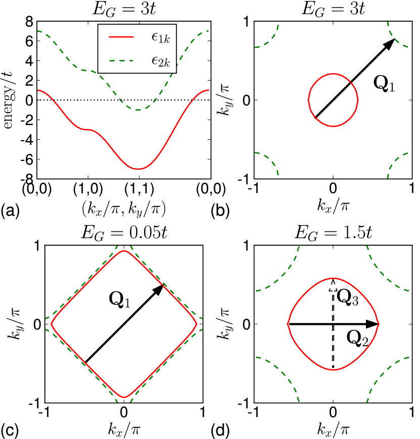
Figure 1: (Color online) (a) Band structure and (b) Fermi surface of the non-interacting model for $t_{1}=t_{2}=t$ and $E_{G}=3\,t$ at half filling. The hole and electron pockets are nested by the vector $\textbf{Q}_{1}=(\pi,\pi)$. The Fermi surfaces for $E_{G}=0.05\,t$ and $E_{G}=1.5\,t$ are shown in (c) and (d), respectively, illustrating the weaker intraband nesting of parts of the electron (hole) Fermi pockets with the vectors $\textbf{Q}_{1}=(\pi,\pi)$, $\textbf{Q}_{2}=(\pi,0)$, and $\textbf{Q}_{3}=(0,\pi)$.

The interaction Hamiltonian consists of three on-site terms which naturally arise in the effective low-energy theory of multi orbital models.CEE2008 Specifically, we have the intraband Coulomb repulsions within each band,

$$H_{U}=\sum_{a=1,2}\frac{U_{aa}}{\mathcal{V}}\sum_{\textbf{k},\textbf{k}^{\prime},\textbf{q}}c_{a\textbf{k}+\textbf{q}\uparrow}^{\dagger}c_{a\textbf{k}^{\prime}-\textbf{q}\downarrow}^{\dagger}c_{a\textbf{k}^{\prime}\downarrow}c_{a\textbf{k}\uparrow},$$ (4)

and the interband Coulomb repulsion,

$$H_{I}=\frac{U_{12}}{\mathcal{V}}\sum_{\textbf{k},\textbf{k}^{\prime},\textbf{q}}\sum_{\sigma,\sigma^{\prime}}c_{1\textbf{k}+\textbf{q}\sigma}^{\dagger}c_{2\textbf{k}^{\prime}-\textbf{q}\sigma^{\prime}}^{\dagger}c_{2\textbf{k}^{\prime}\sigma^{\prime}}c_{1\textbf{k}\sigma}.$$ (5)

For simplicity, we set $U_{22}=U_{11}>0$ in the following, in contrast to previous theoretical studies where the intraband repulsion is neglected.BT2009b ; KECM2010 ; KEM2011 The interband Coulomb repulsion is responsible for the excitonic instability of the nested electron and hole Fermi surfaces. A variety of excitonic mean-field (MF) states are possible, namely charge-, spin-, charge-current-, and spin-current-density waves.B1981 ; JRK1967 ; ZFB2010 For the Hamiltonian Eq. (1), these density-wave states are degenerate, but the ESDW can be stabilized by additional interband correlated-transition terms.B1981 ; BT2009b These terms can be assumed to be arbitrarily small, and so we ignore them in our analysis.

III Mean Field Theory

III.1 Magnetic instabilities of the paramagnetic state

Within the paramagnetic (PM) state, we obtain an effective mean-field Hamiltonian by decoupling the interaction terms in Eq. (1) using the particle densities $n_{a\sigma}=1/\mathcal{V}\sum_{\textbf{k}}\langle c_{a\textbf{k}\sigma}^{\dagger}c_{a\textbf{k}\sigma}\rangle$. We hence find

$$H^{\text{PM}}= \sum_{a=1,2}\sum_{\textbf{k},\sigma}\Big{(}\epsilon_{a\textbf{k}}+U_{aa}n_{a\bar{\sigma}}+U_{12}\sum_{s}n_{\bar{a}s}\Big{)}c_{a\textbf{k}\sigma}^{\dagger}c_{a\textbf{k}\sigma}$$

$$-\sum_{a=1,2}U_{aa}\mathcal{V}n_{a\uparrow}n_{a\downarrow}-U_{12}\mathcal{V}\sum_{\sigma,\sigma^{\prime}}n_{1\sigma}n_{2\sigma^{\prime}},$$ (6)

where we introduce the notation $\bar{a}=2(1)$ when $a=1(2)$. Although we always have perfect nesting, the Hartree terms in Eq. (6) shift the bands relative to one another, thus changing the shape of the Fermi surfaces. It is clear from Figs. 1(b)–1(d) that the changed shape of the Fermi surface may lead to competing magnetic phases. These magnetic instabilities can be determined in an unbiased way by examining the peaks in the PM static spin susceptibility: as the temperature is lowered toward the critical temperature of the magnetic state, the static PM spin susceptibility diverges at the ordering vector Q.

The dynamical spin susceptibility is defined by

$$\chi_{ij,\textbf{q},\textbf{q}^{\prime}}(i\omega_{n})=\frac{1}{\mathcal{V}}\int^{\beta}_{0}d\tau\left\langle T_{\tau}S^{i}_{\textbf{q}}(\tau)S^{j}_{-\textbf{q}^{\prime}}(0)\right\rangle e^{i\omega_{n}\tau},$$ (7)

where $S^{j}(\textbf{q})$ is the spin operator,

$$S^{j}_{\textbf{q}}=\sum_{a,b}S^{j}_{a,b,\textbf{q}}=\frac{1}{\mathcal{V}}\sum_{a,b}\sum_{\textbf{k}}\sum_{s,s^{\prime}}c_{a\textbf{k}+\textbf{q}s}^{\dagger}\frac{\sigma^{j}_{ss^{\prime}}}{2}c_{b\textbf{k}s^{\prime}}.$$ (8)

Inserting Eq. (8) into Eq. (7), we express the spin susceptibility in terms of the generalized susceptibilities,

$$\chi_{ij,\textbf{q},\textbf{q}^{\prime}}(i\omega_{n}) = \sum_{a,b,c,d}\chi_{ij,\textbf{q},\textbf{q}^{\prime}}^{abcd}(i\omega_{n}),$$ (9)

$$\chi_{ij,\textbf{q},\textbf{q}^{\prime}}^{abcd}(i\omega_{n}) = \frac{1}{\mathcal{V}}\int^{\beta}_{0}d\tau\left\langle T_{\tau}S^{i}_{a,b,\textbf{q}}(\tau)S^{j}_{c,d,-\textbf{q}^{\prime}}(0)\right\rangle e^{i\omega_{n}\tau}.$$

We obtain the static transverse MF susceptibilities by making the analytical continuation $i\omega_{n}\rightarrow\omega+i0^{+}$ and then taking the limit $\omega\rightarrow 0$.

Due to the invariance of the PM state under spin rotation, we need only determine the singularities of the transverse spin susceptibility as these contain all information about the possible order in the system. By summing up the ladder diagrams, we obtain the Dyson equation for the generalized RPA spin susceptibilities,

$$\chi^{abba}_{-+,\textbf{q},\textbf{q}}=\chi^{abba(0)}_{-+,\textbf{q},\textbf{q}}+U_{ab}\chi^{abba(0)}_{-+,\textbf{q},\textbf{q}}\chi^{abba}_{-+,\textbf{q},\textbf{q}}.$$ (11)

All other generalized susceptibilities vanish. Expressions for the lowest-order susceptibilities $\chi^{abba(0)}_{-+,\textbf{q},\textbf{q}}$ are found in Ref. BT2009b, . Note that Eq. (11) separates into equations for the interband ($a\neq{b}$) and intraband ($a=b$) spin susceptibilities.

Figure 2: (Color online) Total static transverse spin susceptibility for three representative points of the parameter space for finite temperatures and $t_{1}=t_{2}=t$ and $E_{G}=3t$. Note the different logarithmic scales.

Evaluating the PM spin susceptibility on a $2000\times 2000$ k-point mesh, we find three distinct magnetic instabilities, which we classify by their ordering vector and interband or intraband character.
(i) Interband (excitonic) instability with the ordering vector $\textbf{Q}=\textbf{Q}_{1}$, corresponding to the nesting shown in Fig. 1(b). The evolution of the PM susceptibility is shown in Fig. 2(a). We describe this phase by the order parameter $\Delta_{\sigma\sigma^{\prime}}=(U_{12}/\mathcal{V})\sum_{\textbf{k}}\langle c_{1\textbf{k}\sigma}^{\dagger}c_{2\textbf{k}-\textbf{Q}_{1}\sigma^{\prime}}\rangle$.
(ii) Intraband instability with the ordering vector $\textbf{Q}=\textbf{Q}_{1}$, corresponding to the nesting shown in Fig. 1(c), and the PM susceptibilities in Fig. 2(b). We describe this instability by the order parameter $A_{a\sigma\sigma^{\prime}}^{(1)}=(U_{11}/\mathcal{V})\sum_{\textbf{k}}\langle c_{a\textbf{k}\sigma}^{\dagger}c_{a\textbf{k}-\textbf{Q}_{1}\sigma^{\prime}}\rangle$ with $a=1,2$.
(iii) Intraband instability with the ordering vector $\textbf{Q}=(\alpha,\beta)$, where $\alpha\approx 0$ and $\beta\approx\pi$ or vice versa, corresponding to the nesting shown in Fig. 1(d). To describe this incommensurate (IC) magnetic order we approximate the vectors by $\textbf{Q}_{2}=(\pi,0)$ and $\textbf{Q}_{3}=(0,\pi)$. Typical PM susceptibilities are shown in Fig. 2(c), and we define the order parameters $A_{a\sigma\sigma^{\prime}}^{(\lambda)}=(U_{11}/\mathcal{V})\sum_{\textbf{k}}\langle c_{a\textbf{k}\sigma}^{\dagger}c_{a\textbf{k}-\textbf{Q}_{\lambda}\sigma^{\prime}}\rangle$ with $a=1,2$ and $\lambda=2,3$.

III.2 Mean-field phase diagram

We use the order parameters introduced above and the particle densities $n_{a\sigma}$ to decouple the interaction terms $H_{U}$ and $H_{I}$. Employing standard techniques, we construct the ground-state MF phase diagram, again using a $2000\times 2000$ k-point mesh.

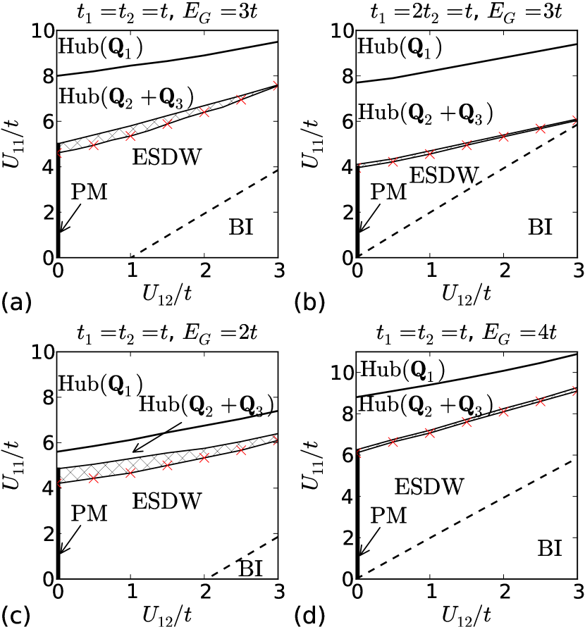
Figure 3: (Color online) Ground-state MF phase diagrams for different parameters of the band structure at half-filling. Solid and dashed lines indicate first-order and second-order phase transitions, respectively. Note that the transition between the $U_{12}=0$ PM and the ESDW phases is of second order. In the shaded region, the MF ground state is the ESDW state, but the static spin susceptibility shows an IC AFM intraband instability above the critical temperature of the ESDW state. The red crosses show points where the critical temperatures of the ESDW and IC AFM states are equal.

Figure 3 shows four ground-state phase diagrams with different values of $E_{G}$ and $t_{2}$. The structure of these phase diagrams is quite similar, implying that the topology of the phase diagram is robust against changes of the band structure. Because of this robustness, we focus on the plot with $t_{1}=t_{2}=t$ and $E_{G}=3\,t$ [Fig. 3(a)]. We find five different phases: the PM phase, the band-insulator (BI) phase, the ESDW phase, the $(\pi,0)+(0,\pi)$ Hubbard AFM phase [$\mathrm{Hub}(\textbf{Q}_{2}+\textbf{Q}_{3})$], and the $(\pi,\pi)$ Hubbard AFM phase [$\mathrm{Hub}(\textbf{Q}_{1})$].

We first consider the phase diagram for weak to moderate $U_{11}\lesssim 5\,t$. At $U_{12}=0$, we find the PM state. Due to the perfect nesting of the electron and hole Fermi pockets, however, only an infinitesimally small $U_{12}$ is required to stabilize the ESDW phase. The Fermi surface is completely gapped, and we have an insulating state. Without loss of generality, we take the SDW polarization to be along the $z$ axis, and so we have the order parameter $\Delta_{\sigma,\sigma^{\prime}}=\sigma\delta_{\sigma,\sigma^{\prime}}\Delta$. Upon increasing $U_{12}$, the Hartree shifts $U_{12}n_{\bar{a}}$ in Eq. (6) push the bands further apart: slightly after the disappearance of the $T=0$ Fermi surface, the ESDW becomes unstable toward the non magnetic BI phase with a completely filled valence and empty conduction band.I2008

Starting in the ESDW phase and increasing $U_{11}$, the Hartree shifts $U_{11}n_{a\bar{\sigma}}$ favor the increase of the occupation of the conduction band, expanding the electron and hole pockets. For $n_{1\sigma}\approx 0.78$, the system undergoes a first-order phase transition into the $\mathrm{Hub}(\textbf{Q}_{2}+\textbf{Q}_{3})$ state with finite order parameters $|A_{a\sigma\sigma^{\prime}}^{(2)}|=|A_{a\sigma\sigma^{\prime}}^{(3)}|\neq 0$ and arbitrary relative sign. This phase is a superposition of magnetically ordered states with intraband ordering vectors $(\pi,0)$ and $(0,\pi)$, and hence possesses a four-site magnetic unit cell. At higher $U_{11}>8t$, the system undergoes another first-order phase transition into the $\mathrm{Hub}(\textbf{Q}_{1})$ state where $A_{a\sigma\sigma^{\prime}}^{(1)}\neq 0$. The existence of this phase is not unexpected because in the limit of $U_{12}=0$ and $U_{11}\gg t,E_{G}$, the system is equivalent to two independent Hubbard models at half-filling.

The cross-shaded area indicates the part of the ground-state phase diagram where the restricted MF calculations predict the ESDW phase but the susceptibilities show an intraband magnetic instability above the critical temperature at an IC wave vector. The existence of IC phases in our two-band model is consistent with results for the single-band Hubbard model away from half-filling.H1985 ; S1990

To summarize, the ESDW state is robust against the intraband interaction up to moderate values of $U_{11}$. Indeed, at these strengths, the Hartree shifts due to the intraband interaction support the ESDW by suppressing the competing BI phase. Magnetic phases mediated by the intraband interaction only appear for $U_{11}\gtrsim 5\,t$. This is the first major result of our work.

IV Transverse Spin Excitations

Figure 4: (a) Logarithm of the imaginary part of the transverse spin susceptibility for $U_{11}=2U_{12}=3.6\,t$ and $\Delta=0.0213\,t$. The spin wave is visible as a dark feature for $\omega<2\Delta$ near $\textbf{q}=\textbf{Q}_{1}$ and $\textbf{q}=\textbf{0}$. Note the logarithmic color scale. (b) Ratio of the total transverse spin susceptibility in panel (a) and the $U_{11}=0$ result presented in Ref. BT2009b, .

The spin excitation spectrum of the ESDW state has unique characteristics which distinguish it from single-band antiferromagnets.BT2009b We obtain the transverse spin susceptibility for the ESDW state within the RPA by summing up the ladder diagrams to all orders. This yields the Dyson equation,

$$\chi^{abcd}_{-+\textbf{q},\textbf{q}^{\prime}}= \delta_{\textbf{q},\textbf{q}^{\prime}}\left(\delta_{a,d}\delta_{b,c}\chi^{abba(0)}_{-+\textbf{q},\textbf{q}^{\prime}}+\delta_{\bar{a},d}\delta_{\bar{b},c}\chi^{ab\bar{b}\bar{a}(0)}_{-+\textbf{q},\textbf{q}^{\prime}}\right)$$

$$+\delta_{\textbf{q}+\textbf{Q}_{1},\textbf{q}^{\prime}}\left(\delta_{\bar{a},d}\delta_{b,c}\chi^{abb\bar{a}(0)}_{-+\textbf{q},\textbf{q}^{\prime}}+\delta_{a,d}\delta_{\bar{b},c}\chi^{ab\bar{b}a(0)}_{-+\textbf{q},\textbf{q}^{\prime}}\right)$$

$$+\sum_{\textbf{p}=\textbf{q},\textbf{q}+\textbf{Q}_{1}}\sum_{m,n=1,2}U_{mn}\chi^{abmn(0)}_{-+\textbf{q},\textbf{p}}\chi^{nmcd}_{-+\textbf{p},\textbf{q}^{\prime}}.$$ (12)

We note that the Dyson equation has been previously obtained in Ref. BT2009b, , where it was solved only for finite non zero interband Coulomb repulsion and all other interactions vanishing.

To calculate the MF transverse spin susceptibilities in Eq. (12), we used a $10000\times 10000$ k-point mesh and a broadening $\delta=10^{-3}t$ in the analytical continuation $i\omega_{n}\rightarrow\omega+i\delta$. Figure 4(a) shows a typical plot of the imaginary part of the transverse spin susceptibility within the ESDW phase for $\textbf{q}=(q_{x},q_{y}=q_{x})$. We set $t_{1}=t_{2}=t$ and $U_{11}=2U_{12}=3.6\,t$, which gives a gap $\Delta=0.0213\,t$. Below, we summarize the main features of the susceptibility; see Ref. BT2009b, for a detailed discussion of the susceptibility for $U_{11}=0$ and $U_{12}=3.6\,t$.

As for the static susceptibility calculated in Sec. III.1, the total transverse spin susceptibility can be divided into contributions from intraband and interband excitations. The former gives the response close to the zone center, while the latter is responsible for the excitations near ${\bf Q}_{1}$. The excitation spectrum shows a partial symmetry of the response about $\textbf{q}=\textbf{Q}_{1}/2$. As shown in Fig. 5(a), the distribution of weight also seems to be a mirror image except for the momenta near $\textbf{Q}_{1}$ and 0. For $\textbf{q}\approx\textbf{0}$, we find a forbidden region which is anticipated by the considered band structure, while there is a significant concentration of weight at $\textbf{q}\approx\textbf{Q}_{1}$.

The excitation spectrum shows a continuum of single-particle excitations for $\omega>2\Delta=0.0426\,t$. This is sharply bounded from below at $\omega=2\Delta$, which is the minimum energy needed to excite quasiparticles across the energy gap of the ESDW state. The spectrum is bounded by V-shaped features at $\textbf{q}\approx 0.54\,\textbf{Q}_{1}$ in the interband susceptibility and at $\textbf{q}\approx 0.46\,\textbf{Q}_{1}$ in the intraband susceptibility. These features are due to the weak nesting of parts of the electron Fermi surface with the hole Fermi surface and with itself, respectively.BT2009b For $\textbf{q}\approx\textbf{Q}_{1}$, we observe a paramagnon line in the interband excitation spectrum. There is a similar but much weaker feature in the intraband susceptibility close to $\textbf{q}=\textbf{0}$.

For $\omega<2\Delta$, a dispersing spin wave is visible close to the magnetic ordering vector and, much more weakly, close to the zone center. The spin-wave dispersion does not intersect with the single-particle continuum, but instead flattens out as it approaches $\omega=2\Delta$ and disappears at $\textbf{q}\approx 0.98\,\textbf{Q}_{1}$ and $\textbf{q}\approx 0.02\,\textbf{Q}_{1}$. Although the paramagnon seems to continue the spin wave into the continuum, closer inspection reveals that the two features avoid each other.

IV.1 Effect of the intraband Coulomb repulsion

As discussed above, the spin excitation spectrum of the ESDW state is qualitatively unchanged by the presence of the intraband Coulomb repulsion. This is unsurprising, as the main features of the transverse susceptibility are fixed by the ESDW state. It is nevertheless interesting to examine the transverse susceptibility for quantitative changes in experimentally relevant details, such as the paramagnon line shape or the spin-wave velocity. A direct comparison with the results of Ref. BT2009b, is nevertheless difficult, as Hartree shifts were not accounted for in that work but instead were assumed to be already included in $E_{G}$. This problem can be avoided, however, by choosing $U_{11}=2U_{12}$, for which the Hartree shifts of the two bands are identical, i.e., effectively vanishing due to the fixed particle concentration. In this case, the band structure in the PM state is the same as the one of the non interacting Hamiltonian.

Figure 4(b) shows the ratio of the transverse spin susceptibility for $U_{11}=2U_{12}=3.6\,t$ and $U_{11}=0$, $U_{12}=1.8\,t$.BT2009b As can be seen, the weight contributed by the intraband components of the spin susceptibility approximately doubles when we include the intraband interaction, while the interband spin susceptibility remains almost the same. Indeed, as shown in Fig. 5(a), the intraband and interband continuum excitations have more nearly equal weight when a finite $U_{11}$ is present. Although the interband contribution is not as dramatically affected, for ${\bf q}\approx{\bf Q}_{1}$ the white line at $\omega>2\Delta$ in Fig. 4(b) indicates a significant suppression of the paramagnon by the intraband Coulomb repulsion, while the white-dark feature at $\omega<2\Delta$ shows a decrease of the spin-wave velocity.

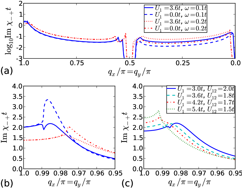
Figure 5: (Color online) (a) Cuts through the excitation spectrum for $U_{11}=0$, $U_{12}=1.8\,t$ and $U_{11}=2U_{12}=3.6\,t$. Note the increase of weight of the susceptibility for $q_{x}<\pi/2$ for $U_{11}\neq 0$, while for $q_{x}>\pi/2$ the weight changes only close to $q_{x}=\pi$. (b) Comparison of the paramagnon line shape for the susceptibilities in (a). The lines are defined as in panel (a). (c) Paramagnon line shape for $\omega=0.1\,t$ and various $U_{11}$ along the line of constant $\Delta=0.0213\,t$ in the phase diagram [see Fig. 6(b)].

We examine the modification of the paramagnon in greater detail in Fig. 5(b). At $U_{11}=0$, the paramagnon can be identified as a distinct peak that becomes broader and lower with increasing energy $\omega$. This changes dramatically at finite $U_{11}$, with the almost complete removal of the peak. At small excitation energies a “peak-dip-hump” structure develops, while at larger energies the paramagnon looks more like a kink. Thus, for fixed normal-state band structure, the intraband interaction can produce a significant change in the paramagnon line shape. In Fig. 5(c), we show the evolution of the paramagnon feature with increasing $U_{11}$, where $U_{12}$ is tuned so that $\Delta$ remains fixed. In contrast to the results in panel (b), here the normal-state Fermi surface undergoes significant changes due to the Hartree shifts. In this case, we see that the “dip-hump” structure disappears with increasing $U_{11}$, leaving only a progressively sharper peak. The strong dependence of the paramagnon line shape on the intraband Coulomb repulsion is the second major result of this paper.

IV.2 Spin-wave velocity

The low-energy dispersion of the spin wave can be analytically obtained by expanding the determinant of the Dyson equation (12) about $\omega=0$ and ${\bf q}={\bf Q}_{1}$. We hence find for the spin-wave dispersion

$$\omega_{\mathrm{m}}(\textbf{Q}_{1}-\textbf{q})=c_{\mathrm{sw}}|\textbf{Q}_{1}-\textbf{q}|,$$ (13)

where $c_{\mathrm{sw}}$ is the spin-wave velocity. For the band structure considered here, we have

$$c_{\mathrm{sw}}^{2}=2a_{3}\,\frac{(1-2U_{11}a_{0})a_{0}-2U_{11}\Delta^{2}a_{1}^{2}}{a_{1}^{2}+2a_{0}a_{2}-8U_{11}a_{0}a_{1}^{2}},$$ (14)

where

$$a_{0} =\frac{1}{4\mathcal{V}}\sum_{\textbf{k}}\frac{\Delta^{2}}{E_{\textbf{k}}^{3}},~{}~{}a_{1}=\frac{1}{4\mathcal{V}}\sum_{\textbf{k}}\frac{\tilde{\epsilon}_{1\textbf{k}}}{E_{\textbf{k}}^{3}},~{}~{}a_{2}=\frac{a_{0}}{2\Delta^{2}},$$ (15)

$$a_{3} =\frac{t}{2\mathcal{V}}\sum_{\textbf{k}}\left(t\,\frac{2\Delta^{2}-\tilde{\epsilon}_{1\textbf{k}}^{2}}{E_{\textbf{k}}^{5}}\,\mathrm{sin}^{2}k_{x}-\frac{\tilde{\epsilon}_{1\textbf{k}}}{2E_{\textbf{k}}^{3}}\,\mathrm{cos}k_{x}\right).$$ (16)

Note that the definition of $a_{3}$ is different from that in Ref. BT2009b, . In the physically relevant limit $\Delta\ll t$, we find

$$c_{\mathrm{sw}}\cong\frac{v_{F}}{\sqrt{2}}\sqrt{1-\mathcal{N}_{0}U_{11}},$$ (17)

where $v_{F}$ is the average Fermi velocity and $\mathcal{N}_{0}$ is the single-spin density of states of one of the bands at the Fermi energy. Equation (17) is the final major result of this work. For $U_{11}=0$, we recover the well-known relation $c_{\mathrm{sw}}\cong v_{F}/\sqrt{2}$.FM1966 ; L1970 ; BT2009b At finite $U_{11}$, the spin-wave velocity can be significantly suppressed by the factor $\sqrt{1-\mathcal{N}_{0}U_{11}}$, and it exactly vanishes when the Stoner criterion for (intraband) ferromagnetism is satisfied. The dependence of the spin-wave velocity on $U_{11}$ can be seen in Fig. 6, where we plot the spin-wave velocity for a cut through the phase diagram at constant order parameter $\Delta$. We find an excellent agreement between Eq. (17) and the numerical data, with the spin-wave velocity going through a maximum as $U_{11}$ is increased. In contrast, the usual expression $c_{\mathrm{sw}}=v_{F}/\sqrt{2}$ overestimates the spin-wave velocity, and monotonically increases with $U_{11}$ due to the effect of the Hartree shifts upon $v_{F}$.

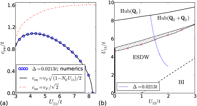
Figure 6: (Color online) (a) Comparison of the numerical (open circles) and the approximate (solid and dash-dotted lines) results for the spin-wave velocity for $\Delta=0.0213\,t$ depending on the intraband Coulomb repulsion. (b) Line of $\Delta=0.0213\,t$ (dash-dotted) for which we determine the spin-wave velocity. We continue the constant-$\Delta$ line to the limit of metastability of the ESDW state within the $\mathrm{Hub}(\textbf{Q}_{2}+\textbf{Q}_{3})$ phase.

V Spin-Wave Velocity in Chromium Alloys

The ESDW state is widely believed to be realized in Cr and its AFM alloys. Cr displays a slightly incommensurate SDW with a Néel temperature of 311 K and a temperature dependence of the staggered magnetization that is well described by standard MF theory.F1988 A commensurate SDW state with much higher $T_{N}$ can be stabilized by doping with Mn.KMTM1966 Several authors have discussed the spin dynamics of such Cr alloys using the RPA.FM1966 ; L1970 ; FL1994 ; FL1996a Neglecting intraband interactions, they found good agreement between theory and experiment above the Néel temperature $T_{N}$.SL1969 ; N1971 At low temperatures $T\ll T_{N}$, a key theoretical prediction is that the spin-wave velocity is $c_{\mathrm{sw}}^{2}=v_{e}v_{h}/3$, where $v_{h(e)}$ is the hole (electron) Fermi velocity and the factor of $3$ in the denominator arises because a three-dimensional band structure is considered.FL1994 ; L1970 ; FM1966 ; FL1996a Experiments, however, show that this result overestimates $c_{\mathrm{sw}}$ by a factor of approximately 2.SL1969 ; N1971 ; SK1977 This discrepancy persists in more sophisticated models of the band structure (e.g., Ref. FL1996a, ) and has not yet been conclusively explained. A notable attempt was made by Liu, L1976 ; L1981 who proposed that the coupling between SDW-induced local moments on the Cr ions and magnons was responsible for the reduced spin-wave velocity.

In Sec. IV, we found that the intraband Coulomb repulsion provides a significant renormalization of the spin-wave velocity in the ESDW phase. It is therefore interesting to estimate the effect of this renormalization for Mn-doped Cr alloys [the result, Eq. (17), can easily be generalized to a three-dimensional system by replacing the factor $\sqrt{2}$ by $\sqrt{3}$]. Ab initio calculations estimate the total density of states of paramagnetic Cr to be approximately $0.65$ eV^-1.S1981 ; LCFB1981 Ignoring non-nested portions of the Fermi surface, this gives an upper bound ${\cal N}_{0}\lesssim 0.16$ eV^-1. LiuL1970 estimated ${\cal N}_{0}U_{12}=0.43$ by fitting to experimental data on Cr_0.98Mn_0.02. It is therefore reasonable to take $U_{11}\approx 3\,$eV, which gives a renormalization $\sqrt{1-\mathcal{N}_{0}U_{11}}\approx 0.7$, i.e., the renormalization factor yields a reduction of the spin-wave velocity by approximately 30 %. This accounts for the bulk of the discrepancy between the $U_{11}=0$ theory and experimental findings, and suggests that the hitherto neglected intraband interactions could play a significant role in the spin dynamics of Cr and its alloys. We note that a finite $U_{11}$ will not affect the low-energy normal-state spin dynamics near to the magnetic ordering vector, and so the previous results for $T>T_{N}$ are also valid in our theory.

VI Conclusions

In this paper, we have presented an analysis of a two-dimensional two-band Hubbard model with nested electron and hole Fermi surfaces. By examining the static RPA spin susceptibility in the paramagnetic state, we have determined the possible magnetic order in an unbiased way. In addition to the expected interband ESDW, we have found instabilities toward a number of intraband AFM states with various commensurate and incommensurate ordering vectors. Using these results to inform a mean-field ansatz, we have calculated the ground-state phase diagram for a number of different semimetallic band structures. We have shown that the ESDW state is stable at weak to moderate intraband coupling; at stronger interaction strengths, however, changes in the Fermi surface induced by the Hartree shifts stabilize the intraband AFM states.

In the second part of the paper, we have studied the effect of the intraband interactions on the low-temperature spin dynamics of the ESDW. We have solved the Dyson equation for the transverse spin susceptibility and have compared the results for vanishing BT2009b and finite intraband interactions. We find that there is significant renormalization of key experimentally relevant details of the spin excitation spectrum due to intraband interactions. Specifically, the intraband interactions qualitatively alter the paramagnon line shape and reduce the spin-wave velocity. We argue that this mechanism could resolve the discrepancy between the measured spin-wave velocity in Mn-doped Cr and previous theoretical predictions.

- (1) Y. Kamihara, T. Watanabe, M. Hirano, and H. Hosono, J. Am. Chem. Soc. 130, 3296 (2008).
- (2) J. Paglione and R. L. Green, Nature Phys. 6, 645 (2010).
- (3) M. D. Lumsden and A. D. Christianson, J. Phys.: Condens. Matter 22, 203203 (2010).
- (4) C. de la Cruz, Q. Huang, J. W. Lynn, J. Li, W. Ratcliff II, J. L. Zaretsky, H. A. Mook, G. F. Chen, J. L. Luo, N. L. Wang, and P. Dai, Nature (London) 453, 899 (2008).
- (5) S. E. Sebastian, J. Gillett, N. Harrison, P. H. C. Lau, C. H. Mielke, and G. G. Lonzarich, J. Phys.: Condens. Matter 20, 422203 (2008).
- (6) M. Yi, D. H. Lu, J. G. Analytis, J.-H. Chu, S.-K. Mo, R.-H. He, M. Hashimoto, R. G. Moore, I. I. Mazin, D. J. Singh, Z. Hussain, I. R. Fisher, and Z.-X. Shen, Phys. Rev. B 80, 174510 (2009).
- (7) D. J. Singh and M.-H. Du, Phys. Rev. Lett. 100, 237003 (2008).
- (8) I. I. Mazin, D. J. Singh, M. D. Johannes, and M. H. Du, Phys. Rev. Lett. 101, 057003 (2008).
- (9) R. A. Ewings, T. G. Perring, J. Gillett, S. D. Das, S. E. Sebastian, A. E. Taylor, T. Guidi, and A. T. Boothroyd, Phys. Rev. B 83, 214519 (2011).
- (10) D. K. Pratt, M. G. Kim, A. Kreyssig, Y. B. Lee, G. S. Tucker, A. Thaler, W. Tian, J. L. Zarestky, S. L. Bud’ko, P. C. Canfield, B. N. Harmon, A. I. Goldman, and R. J. McQueeney, Phys. Rev. Lett. 106, 257001 (2011).
- (11) Q. Han, Y. Chen, and Z. D. Wang, Europhys. Lett. 82, 37007 (2008).
- (12) M. M. Korshunov and I. Eremin, Phys. Rev. B 78, 140509(R) (2008).
- (13) A. V. Chubukov, D. V. Efremov, and I. Eremin, Phys. Rev. B 78, 134512 (2008).
- (14) V. Cvetkovic and Z. Tesanovic, Europhys. Lett. 85, 37002 (2009); Phys. Rev. B 80, 024512 (2009).
- (15) A. B. Vorontsov, M. G. Vavilov, and A. V. Chubukov, Phys. Rev. B 79, 060508(R) (2009).
- (16) P. M. R. Brydon and C. Timm, Phys. Rev. B 79, 180504(R) (2009).
- (17) P. M. R. Brydon and C. Timm, Phys. Rev. B 80, 174401 (2009).
- (18) J. Knolle, I. Eremin, A. Akbari, and R. Moessner, Phys. Rev. Lett. 104, 257001 (2010).
- (19) J. Knolle, I. Eremin, A. V. Chubukov, and R. Moessner, Phys. Rev. B 81, 140506(R) (2010).
- (20) R. M. Fernandes and J. Schmalian, Phys. Rev. B 82, 014521 (2010).
- (21) S. Maiti and A. V. Chubukov, Phys. Rev. B 82, 214515 (2010).
- (22) J. Knolle, I. Eremin, and R. Moessner, Phys. Rev. B 83, 224503 (2011).
- (23) J. des Cloizeaux, J. Phys. Chem. Solids 26, 259 (1965).
- (24) L. V. Keldysh and Y. V. Kopaev, Fiz. Tverd. Tela (Leningrad) 6, 2791 (1964) [Sov. Phys. Solid State 6, 2219 (1965)].
- (25) A. N. Kozlov and L. A. Maksimov, Zh. Eksp. Teor. Fiz. 48, 1184 (1965) [Sov. Phys. JETP 21, 790 (1965)].
- (26) D. Jerome, T. M. Rice, and W. Kohn, Phys. Rev. 158, 462 (1967).
- (27) J. Zittartz, Phys. Rev. 162, 752 (1967).
- (28) F. X. Bronold and H. Fehske, Phys. Rev. B 74, 165107 (2006).
- (29) T. M. Rice, Phys. Rev. B 2, 3619 (1970).
- (30) P. A. Fedders and C. A. Martin, Phys. Rev. 143, 245 (1966).
- (31) S. H. Liu, Phys. Rev. B 2, 2664 (1970).
- (32) D. W. Buker, Phys. Rev. B 24, 5713 (1981).
- (33) K. Machida and M. Fujita, Phys. Rev. B 30, 5284 (1984).
- (34) E. Fawcett, Rev. Mod. Phys. 60, 209 (1988).
- (35) R. S. Fishman and S. H. Liu, Phys. Rev. B 50, 4240(R) (1994).
- (36) R. S. Fishman and S. H. Liu, Phys. Rev. B 54, 7233 (1996).
- (37) A. I. Rusinov, D. C. Kat, and Y. V. Kopaev, Zh. Eksp. Teor. Fiz. 65, 1984 (1973) [Sov. Phys. JETP 38, 991 (1974)]; M. Gulácsi and Zs. Gulácsi, Phys. Rev. B 39, 714 (1989).
- (38) B. Zenker, H. Fehske, and C. D. Batista, Phys. Rev. B 82, 165110 (2010).
- (39) D. Ihle, M. Pfafferott, E. Burovski, F. X. Bronold, and H. Fehske, Phys. Rev. B 78, 193103 (2008).
- (40) J. E. Hirsch, Phys. Rev. B 31, 4403 (1985).
- (41) H. J. Schulz, Phys. Rev. Lett. 64, 1445 (1990).
- (42) W. C. Koehler, R. M. Moon, A. L. Trego, and A. R. Mackintosh, Phys. Rev. 151, 405 (1966).
- (43) S. K. Sinha, S. H. Liu, L. D. Muhlestein, and N. Wakabayashi, Phys. Rev. Lett. 23, 311 (1969).
- (44) J. Als-Nielsen, J. D. Axe, and G. Shirane, J. Appl. Phys. 42, 1666 (1971).
- (45) S. K. Sinha, G. R. Kline, C. Stassis, N. Chesser, and N. Wakabayashi, Phys. Rev. B 15, 1415 (1977).
- (46) S. H. Liu, Phys. Rev. B 13, 3962 (1976).
- (47) S. H. Liu, J. Magn. Magn. Mater. 25, 97 (1981).
- (48) H. L. Skriver, J. Phys. F 11, 97 (1981).
- (49) D. G. Laurent, J. Callaway, J. L. Fry, and N. E. Brener, Phys. Rev. B 23, 4977 (1981).