Construction of Complete Embedded Self-Similar Surfaces under Mean Curvature Flow. Part III.
Abstract.
We present new examples of complete embedded self-similar surfaces under mean curvature flow by gluing a sphere and a plane. These surfaces have finite genus and are the first examples of non-rotationally symmetric self-shrinkers in . Although our initial approximating surfaces are asymptotic to a plane at infinity, the constructed self-similar surfaces are asymptotic to cones at infinity.
Key words and phrases:
mean curvature flow, self-similar, singularities, solitons2000 Mathematics Subject Classification:
Primary 53C441. introduction
This article is the third and last installment of a series of papers aiming at constructing new examples of surfaces satisfying the self-shrinking equation for the mean curvature flow,
| (1) |
where is the position vector, the function and the orientation of the unit normal are taken so that the mean curvature vector is given by .
In [8], Huisken proved that if the growth of the second fundamental form is controlled (type 1), the singularities of the mean curvature flow tend asymptotically to a solution to (1). The work on self-shrinking surfaces is therefore motivated by a desire to better understand the regularity of the mean curvature flow. A long list of examples of self-shrinkers would help shed light on the behavior of the flow near its singularities; unfortunately, until now, there were only four known examples of complete embedded self-shrinking surfaces (in the Euclidean space ): a plane, a cylinder, a sphere, and a shrinking doughnut [1]; although there is numerical evidence of many others [2][3].
The overarching idea in the three articles is to obtain new examples of self-shrinkers by desingularizing the intersection of two known examples (the sphere of radius centered at the origin and a plane through the origin) using Scherk minimal surfaces. First, one constructs an initial approximate solution by fitting an appropriately bent and scaled Scherk surface in a neighborhood of the intersection, then one solves a perturbation problem in order to find an exact solution. The method was successfully used by Kapouleas [10] and Traizet [23] to construct minimal surfaces, and by the author for self-translating surfaces under the mean curvature flow [18] [20].
The main difficulty in these desingularizations lies in showing that the linearized equation can be solved on the initial surface . One attacks it by studying on smaller pieces first. In the first article [17], we study the linearized equation on the desingularizing surface . The second article concerns the outer plane (the plane with a central disk removed) and its main result states that the Dirichlet problem for (1) on has a unique solution among graphs of functions over with a controlled linear growth. In the present article, we finish the construction by gluing the solutions to the linearized equations on the different pieces to obtain a global solution with a standard method: we use cut-off functions to localize the inhomogeneous term to the different pieces, solve the linearized equation on these pieces, glue the local solutions using cut-off functions again, and iterate the process. However, the cut-off functions create errors and obtaining the right estimates for the iteration to converge requires a delicate and precise construction of the initial approximate surfaces, which is the main focus of this article.
Once the initial surfaces are constructed, the techniques from [10] can be readily applied, with one notable exception. In all the previous constructions [10], [23], [18], and [20], the surfaces converge exponentially to their asymptotic catenoids, planes, or grim reapers respectively. But here, the self-shrinkers grow linearly at infinity. In this article, we also refine previous estimates from [19] and define the appropriate Banach spaces of functions for the final fixed point theorem.
The author originally intended to desingularize the intersection of a cylinder and a plane, inspired by the work of Kapouleas on minimal surfaces and Ilmanen’s open problem on the rigidity of the cylinder. In [9], Ilmanen conjectured that if one of the ends of a self-shrinking surface is asymptotic to a cylinder, then the surface must be the self-shrinking cylinder itself. At the time, Angenent suggested that the desingularization of a cylinder and a plane could provide a counterexample. The problem was harder than anticipated because of the asymptotic behavior along the cylindrical ends and remains open. In the same set of lecture notes, Ilmanen predicted the existence of self-shrinking punctured saddles, which he called -saddles, and provided pictures for and . Theorem 1 below shows that these -saddles exist if is large; the existence for small is still an open problem. The parameter is the number of periods of a Scherk surface needed to wrap around the intersection circle. The -saddle below therefore has handles and genus .
Theorem 1.
There exists a natural number so that for any natural number , there exists a surface with the following properties:
-
(i)
is a complete smooth surface which satisfies the equation .
-
(ii)
is invariant under rotation of around the -axis.
-
(iii)
is invariant under reflections across planes containing the -axis and forming angles , , with the -axis.
-
(iv)
Let be the open top half of the ball of radius . As , the sequence of surfaces tends to the sphere of radius centered at the origin on any compact set of .
-
(v)
is asymptotic to a cone.
-
(vi)
If we denote by the translation by the vector , the sequence of surfaces converges in to the original Scherk surface on compact sets, for all .
We briefly sketch the proof below, highlighting the differences and similarities between this construction and the ones from [10] and [20].
We start by replacing a small neighborhood of the intersection circle by an appropriately bent Scherk surface to obtain embedded surfaces. However, instead of scaling down the Scherk surface by a factor where is a small positive constant, we keep it in its natural scale so that the curvatures and second fundamental form stay bounded, and scale up the rest of the configuration by . The equation to be satisfied is then
| (2) |
These initial surfaces are embedded and will be our approximate solutions. The next and more difficult step consists in finding an exact solution among perturbations of the initial surfaces. More precisely, we perturb a surface by adding the graph of a small function so the position vector becomes . Denoting the initial surface by , its position vector by , its unit normal vector by , the graph of over by , its mean curvature by , and its unit normal vector by , we have
where is the second fundamental form on and is at least quadratic in , , and . The surface is a self-shrinker if
| (3) |
where . Once we can solve the equation , we expect the quadratic term to be small so the solution to (3) could be obtained by iteration. Before we can solve the linearized equation on the initial surface , we have to study its associated Dirichlet problem on the various pieces: the desingularizing surface (formed by a truncated bent Scherk surface), the two rotationally symmetric caps , the inner disk , and the outer plane .
In all of the previous constructions (and here also), the linear operator has small eigenvalues on . One way to deal with the presence of small eigenvalues is to restrict the class of possible perturbations and eigenfunctions by imposing symmetries on all the surfaces considered. However, this method only works if the initial configuration has the imposed symmetries and, in general, can not rule out all the troublesome eigenfunctions. A second complementary approach is to invert the linear operator modulo the eigenfunctions corresponding to small or vanishing eigenvalues. In other words, one can add or subtract a linear combination of eigenfunctions to the inhomogeneous term of in order to land in the space perpendicular to the approximate kernel, where the operator has a bounded inverse. For an exact solution, one must be able to generate (or cancel) any linear combination of these eigenfunctions within the construction. The process is called unbalancing and consists in dislocating the Scherk surface so that opposite asymptotic planes are no longer parallel. Flexibility in the initial configuration is the key to a successful construction. The terms unbalancing and flexibility were first introduced by Kapouleas and the reader can find a short discussion of them in the survey article [11].
1.1. How this construction differs from previous ones.
In [10] ([20]), the flexibility relies on the fact that the main equation ( resp.) is translation invariant, so the catenoidal ends (grim reaper ends resp.) could be shifted without creating errors. Moreover, since catenoids (grim reapers resp.) have ends, one can, with careful planning, perform the required dislocation at the intersections so that all the small changes in position build up toward loose ends. For the case of self-shrinkers, the sphere of radius centered at the origin is the only sphere satisfying (1) so the apparent lack of flexibility has been a major impediment in completing the desingularization of the sphere and the plane.
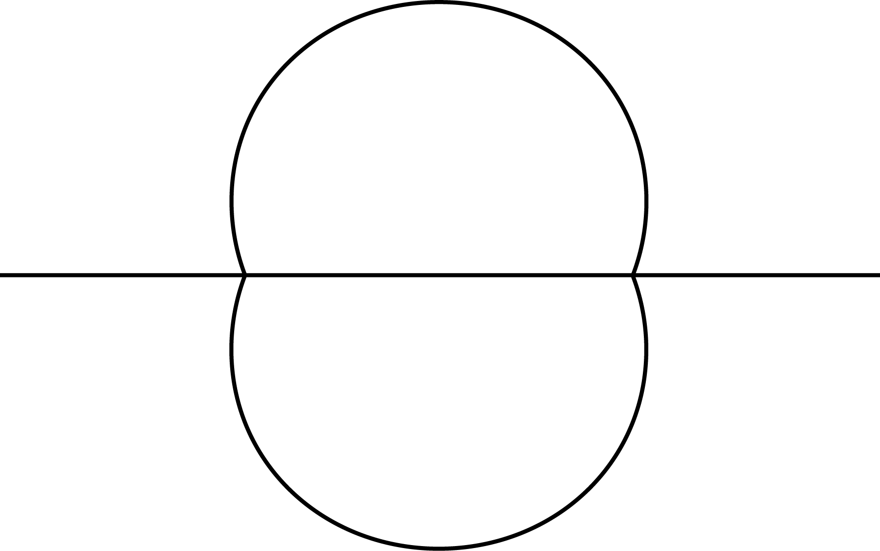
The unbalancing process requires one to consider the configuration of a sphere and a plane as part of a family of initial configurations in which the rotationally symmetric caps meet the plane at various angles close to degrees (see Figure 1 for a dramatized representation).

Rather than shifting the sphere up or down, which would create too much error, we use a family of self-shrinking rotationally symmetric caps. In [1], Angenent showed that rotationally symmetric self-shrinkers are generated by geodesics in the half-plane with metric
| (4) |
The equation for these geodesics parametrized by arc length is given by the following system of ordinary differential equations:
| (5) |
where is the tangent angle at the point .
The metric is degenerate, so generic geodesics will bounce off as they get close to the -axis. To obtain smooth embedded caps for the construction, we have to select only the geodesics that tend to the -axis (and which will eventually become perpendicular to the -axis). They form a one parameter family of solutions to (5) characterized by the initial conditions , , and . Because of the metric, the existence and uniqueness of such solutions do not follow from standard ODE methods but from the (un)stable manifold theorem. The flexibility here comes from this one parameter family of rotationally symmetric self-shrinking caps; and a prescribed unbalancing dictates which cap to select and the radius of the intersection circle.
The asymptotic behavior of our self-shrinkers is also different from the previous constructions in [10] and [20]. In both of these articles, the constructed examples tended exponentially fast to the asymptotic catenoids or grim reapers. In this case, although the initial configurations all involve the -plane, the constructed self-shrinkers are asymptotic to cones at infinity [19].
1.2. How this construction is similar to previous ones.
In [10] and [20], the desingularizing surfaces were not only unbalanced but their wings were bent as well to ensure that the solutions to the linearized equation could be adjusted to have exponential decay. The decay is crucial to control the error generated from the cut-off functions when patching up the local solutions to the linearized equation to form a global solution. In this construction, we can impose an added invariance with respect to the half-turn rotation about the -axis, and this extra symmetry forces exponential decay on the solutions along the wings of the desingularizing Scherk surface. The situation is similar to the one in [18] and we do not need any bending of the wings.
All the estimates and results about the linearized equation on the desingularizing surface are obtained by arguments analogous to the ones in [10], although our construction is simpler because there is no bending. Indeed, the difference between equation (2) and is of order and the respective linear operators also differ by terms of order at least . Since the proofs are very technical and not enlightening, we will not repeat them in this article but just state the relevant properties. The reader who wishes more details can find some in [18], where we adapted all of the proofs for the equation . At this point, we would like to warn the reader that this article is not self-contained and we rely on the reader’s familiarity with similar constructions, especially [10] or [18], for the proofs of Propositions 8 and 15.
Once we define the correct Banach spaces of functions and norms to consider, the few last steps in this article are similar to the ones from Kapouleas’s. Namely, the proof that the linearized equation on the initial surface can be solved modulo a multiple of a well-chosen function follows the same lines as in Kapouleas’ article. The final fixed point argument is also similar. Because it would have been strange to stop the construction right before its conclusion, we have included these proofs for the sake of completeness.
Acknowledgments
The author would like to thank Sigurd Angenent for introducing her to this problem and for his encouragement to persist in solving it.
The author would also like to thank the referees for helpful comments in clarifying the presentation of this article. They have also pointed out that even though all the essential ideas and estimates were present in Section 5.4, the weighted Hölder norms defined in the original version did not yield the compact embeddings necessary to apply the Schauder Fixed Point Theorem. The error has been corrected in this version with the addition of Definition 21 and Lemma 22.
The original version of this article contained an extra parameter for bending the wings of the desingularizing surfaces. The imposed invariance under rotation of around the -axis makes superfluous and the author has removed it.
After completion of the original manuscript, the author learned that N. Kapouleas, S. Kleene, and N. Møller have announced a similar result [12]. They tackled both points mentioned in the previous two paragraphs correctly in their first version.
Remark
The notation (which makes the unit inward normal vector for convex surfaces) and the particular scale (in which the sphere of radius in is a solution to the self-shrinker equation) follow the conventions of the previous two installments [17] and [19]. The scale differs from the scale in Angenent [1], where the sphere of radius is self-shrinking. It is also worth noting that the orientation of our normal vector is opposite from the one chosen by Huisken in [8].
1.3. Notation
-
•
is the Euclidean three space equipped with the usual metric.
-
•
, and are the three coordinate vectors of .
-
•
We fix once and for all a smooth cut-off function , which is increasing, vanishes on , and is equal to on . We define the functions which transition from at to at by
-
•
We often have a function defined on the surfaces with values in . If is a subset of such a surface, we use the notation
-
•
, and denote, respectively, the oriented unit normal vector, the induced metric, the second fundamental form, and the mean curvature of an immersed surface in the Euclidean space .
-
•
Given a surface in , which is immersed by and a function , we call the graph of over the surface given by the immersion , and denote it by . We often use and its inverse to define projections from to , or from to , respectively. When we refer to projections from to or from to , we always mean these projections.
-
•
Throughout this article, a surface with a tilde is a surface in the “smaller” scale, whereas a surface without a tilde denotes its “larger” version , where is a small positive constant. We also use these conventions for geometric quantities, for example, is the mean curvature of and is the mean curvature of . However, these notations apply only loosely to coordinates: we generally use when we are working in a “larger” scale and for objects in a “smaller” scale but these sets of coordinates are not necessarily proportional by a ratio of .
-
•
We work with the following weighted Hölder norms:
where is a domain, is the metric with respect to which we take the norm, is the weight function, and is the geodesic ball centered at of radius .
2. Construction of the desingularizing surfaces
We introduce the Scherk minimal surface and describe how to unbalance, wrap, and bend it to obtain a suitable desingularizing surface. The parameter is a small positive constant which characterizes how much the desingularizing surface will be scaled to fit in the neighborhood of the intersection circle. Although we do not scale the desingularizing surface in this section, still plays a role here as it determines the radius of the circle around which the Scherk surface is wrapped, and how far we truncate our surface.
2.1. The Scherk surface
The Scherk minimal surface is given by the equation
This surface was discovered by Scherk and is the most symmetric of a one parameter family of minimal surfaces (see [4], [13], or [14]). As () goes to infinity, tends exponentially to the -plane (-plane resp.). More precisely, if we denote by the closed half-plane , we have the following properties.
Lemma 2 (Proposition 2.4 [10]).
For given , there are a constant and smooth functions and with the following properties:
-
(i)
,
-
(ii)
,
-
(iii)
is invariant under rotation of around the -axis, and reflections across the planes , .
The constant is a small constant chosen at this point so is also fixed. We call the surface the top wing of , and its image under rotation of around the -axis is the bottom wing. The outer wing is the set of points and the inner wing is . We take as standard coordinates the coordinates on each of the wings. If a point of does not belong to any of the wings, we take its -coordinate to be zero.
2.2. Unbalancing
Because the equation is a perturbation of , one expects that the respective linear operators and have similar properties. The mean curvature is invariant under translations, therefore the functions , , and are in the kernel of the linear operator associated to normal perturbations of . We can rule out and by imposing symmetries (see (iii) of Lemma 2). The remaining function does not have the required exponential decay, however, it indicates that has an approximate kernel generated by a function close to and one can only solve the equation with a reasonable estimate on if is perpendicular to the approximate kernel. But we do not have such control over the inhomogeneous term, so we have to introduce a function to cancel any component parallel to the approximate kernel. The function has to be in the direction of in the sense that .
Let be one period of the desingularizing surface . According to the balancing formula from [15], the mean curvature of satisfies
where is the direction of the plane asymptotic to the th wing. The idea is to define as a derivative of and use unbalancing to move the top and bottom wings toward to generate a multiple of .
Definition 3.
For , we take a family of diffeomorphisms depending smoothly on and satisfying the following conditions:
-
(i)
is the identity in the region ,
-
(ii)
in the region , is the rotation by an angle about the -axis toward the positive -axis,
-
(iii)
is the identity.
We denote by the unbalanced surface and push forward the coordinates of onto this new surface using .
2.3. Wrapping the Scherk surface around a circle
Given , let and define the maps by
We allow to differ slightly from so that it can be chosen to fit the self-shrinking rotationally symmetric caps in Section 4.2. The exponential factor has no real significance here and can be replaced by any strictly increasing diffeomorphism with the property .
We push forward the coordinates of onto the surface . The piece of surface corresponding to within the slab is called the core of the desingularizing surface and will no longer be modified. The image of the plane asymptotic to the top wing of is given by
| (6) |
where we placed the boundary of the asymptotic surface at to simplify subsequent computations. In general, the piece of sphere given by (6) does not satisfy the equation for self-shrinkers (1) and would generate too much error if it were used to build the top wing. Instead, we record its boundary and conormal direction in Definition 4 and equation (7), respectively, then choose a piece of rotationally self-shrinking surface these boundary conditions in Definition 5.
Definition 4.
The circle that bounds the asymptotic surface given by (6) is called the pivot of the top wing.
We define to be the angle the inward conormal vector makes with the direction at the pivot, which is given by the equation
| (7) |
Note that is a smooth function of and that for some positive constant .
Definition 5.
From standard ODE theory, the flow of (5) is smooth and depends smoothly on the initial conditions. The surfaces are not embedded in general, but we only consider the small pieces where , where the small positive constant will be determined in Section 3. The pull-back of the induced metric by is where
2.4. The inner and outer wings
The construction of these two wings is very simple: we just use the transition function to cut off the graph of over these two wings, then truncate the desingularizing surface at .
2.5. The top and bottom wings.
The top wing of our desingularizing surface is essentially the graph of from Lemma 2 over the self-shrinking rotationally symmetric surface . To get smooth transitions, we use the cut-off functions and . The factor in the scale of is to ensure that we cut off far enough as not to generate too much error, while is small in order to control the geometry of the wings and so that the desingularizing surfaces fit in a small neighborhood of the intersection circle (in the original scale of (1)).
Definition 6.
For given , and as in Definition 5, we define by
where is defined by and is the Gauss map of chosen so that
The top wing is divided into four regions:
-
•
is a transition region from the core to the bent wing.
-
•
on , the wing is the graph of over the asymptotic rotationally symmetric piece of self-shrinker.
-
•
is another transition region where we cut off the graph of .
-
•
on , the wing is a piece of rotationally symmetric self-shrinker.
As before, we push forward the coordinates of onto and clip the wing at . The bottom wing is obtained by rotating the top wing by around the -axis.
2.6. The desingularizing surfaces
The desingularizing surface is composed of the core, the inner and outer wings, and the top and bottom wings defined in the three previous sections. We sometimes denote it by for simplicity. The next proposition collects some useful properties of our desingularizing surfaces.
Proposition 7.
There exists a constant such that for , , and , the surface satisfies the following properties:
-
(i)
is a smooth surface immersed in which depends smoothly on its parameters.
-
(ii)
If , , the surface is embedded. Moreover, is invariant under the rotation of around the -axis and under the reflections across planes containing the -axis and forming angles , , with the -plane.
3. Estimates on the desingularizing surfaces
In this section, we claim that the desingularizing surfaces are suitable approximate solutions. All the estimates from Section 4 in [10] are valid, with replaced by and the corresponding linear operator replaced by . The factor combats the scale of the position so the extra term does not add significantly. This is where we choose the constant small enough so that the metrics , , and are uniformly equivalent on the top and bottom wings. Later on, in the proof of Proposition 15, may be changed to an even smaller constant so that the linear operator on the wings can be treated as a perturbation of the Laplace operator on a flat cylinder. Because the proofs are technical and do not showcase the main aspects of the construction, we will not reproduce them here. The reader can find all the details in Section 4 of [10] or Section 3 of [18].
In what follows, the parameter and the radius are fixed and the dependence on will be omitted. Moreover, because takes values in a compact set, all of the constants can be chosen independently of .
We define the function by
where denotes the mean curvature on the surface .
The main contribution to comes from the unbalancing term (). Here is a constant in which indicates that the exponential decay is slower due to the presence of the cut-off function in Definition 6.
Proposition 8.
For as in Proposition 7, the quantity on satisfies
4. Construction of the initial surfaces
In the construction of the desingularizing surfaces, we did not unbalance or bend the inner and outer wings so attaching them to a disk and plane respectively is straightforward. For the top and bottom wings, the story is more complicated. In the case of minimal surfaces, coaxial catenoids form a two parameter family of minimal surfaces whose embeddings depend smoothly on the parameters. When the desired tangent direction of a gluing wing is changed, one has the flexibility of attaching a catenoid close to the original one. To get flexibility in this construction, we have to consider the sphere of radius as a member of a family of self-shrinking surfaces and not as a member of a family of spheres. Note that in [10], Kapouleas had invariance for reflection across planes only, so he used a two-parameter family of initial configurations. Since we have an additional symmetry (invariance under rotation of around the -axis), the family of self-shrinking surfaces depends on one parameter only.
4.1. A family of rotationally symmetric self-shrinking caps
In [1], Angenent showed that hypersurfaces of revolution are self-shrinkers if and only if they are generated by geodesics of the half-plane equipped with the metric (4). Given any point and an angle , there is a unique geodesic through with tangent vector . Such a geodesic parametrized by arc length satisfies the following system of ODEs
| (5) |
Because the metric becomes degenerate as , geodesics in general will bounce off as they approach the -axis. For the purpose of having a complete rotationally symmetric cap, we will only consider geodesics that tend towards the -axis. Such curves will always meet the -axis at a right angle.
Definition 9.
For close to , we denote by or the geodesic in the half-plane equipped with the metric (4) with initial conditions
Note that the curve is the projection to the -plane of the solution to (5) with initial conditions
The solution corresponding to the hemisphere of radius is
Proposition 10.
There exists a constant for which the map that associates to in Definition 9 is smooth.
The number was chosen so that all the geodesics would exist long enough to exit the first quadrant.
Proof.
The system of ODEs (5) can be reparametrized using the variable for which to get
With this parametrization in the octant ,
-
•
the line is invariant (and the corresponding self-shrinker is the plane),
-
•
the line is invariant (and the corresponding self-shrinker is the cylinder),
-
•
the line consists of fixed points. The linearization at is
The line is therefore normally hyperbolic, with a stable manifold contained in the plane . Its unstable manifold consists of a one parameter family of orbits , each emanating from the point . The short-time existence and uniqueness of these orbits , as well as the smoothness of the unstable manifold is given by the (un)stable manifold theorem (see Theorem (4.1) [7] or Theorem III.8 [21]). Once we get away from the line using this first step, we can extend the one parameter family of orbits smoothly using standard ODE theory. The uniform dependence of for is obtained by a compactness argument since the system (5) is not singular for away from zero. ∎
Proposition 11.
There exists a positive constant such that given there exists a unique constant for which the orbit hits the -axis at an angle . Moreover, for some constant independent of , we have
Proof.
We start the proof by giving a different description of the geodesics. The graph of a function over the circle of radius , i.e. the curve given by , is a self-shrinker if and only if
Using the change of variable , the equation above is equivalent to
The existence of a solution with , follows from the proof of Proposition 10. In addition, the unstable manifold theorem gives the smooth dependence of the solution on its parameters and
where as and where the function satisfies the linear ODE
The solution is given by , where is the Legendre function. We get the existence of and the estimate (8) below because the derivative is positive at . ∎
In the following corollary, we seek to hit the line at a specific angle .
Corollary 12.
There exists a positive constant independent of such that given with
there exists a unique constant for which the orbit hits the line at an angle and
| (8) |
4.2. Fitting the self-shrinking caps to the desingularizing surfaces
Let us recall that in Section 2, we did not restrict ourselves to geodesics that meet the -axis perpendicularly but considered any solution to (5) to construct the asymptotic surfaces . We now choose the radius in function of the angle so that the surface asymptotic to the top wing of is contained in a self-shrinking rotationally symmetric cap. Given , we take to be the given in Corollary 12 corresponding to , where is given by (7).
4.3. Construction of the initial surfaces
Let us recall that , for a previously chosen integer . We fix a constant which will be determined in the proof of Theorem 1.
Given , we start the construction of the initial surface by taking the desingularizing surface and shrinking it to with the homothety of ratio centered at the origin. We top off (on the top and bottom) the desingularizing surface with self-shrinking caps generated by rotating the curve around the -axis. The inner wing of is attached to a flat disk and the outer wing to a plane.
Definition 13.
The surface constructed in the above paragraph is denoted by . We push forward the function by from to and extend it to the whole surface by taking on .
Let . We define
and their image under by , and respectively.
Choosing the constant of order will be useful for getting a contraction (equation (21)) in the proof of Theorem 24.
Proposition 14.
Given a positive integer so that and , the surface is well defined by the construction above and satisfies the following properties:
-
(i)
is a complete smooth embedded surface which depends smoothly on .
-
(ii)
is invariant under rotation of around the -axis.
-
(iii)
is invariant under the action of the group generated by reflections across the planes containing the axis and forming an angle of , with the -plane.
-
(iv)
As , the sequence of initial surfaces converges uniformly in , for all , to the union of a sphere of radius and the -plane on any compact subset of the complement of the intersection circle.
-
(v)
Let us denote by the translation by the vector . As , the sequence of surfaces converges uniformly in , for all , to the Scherk surface on any compact subset of .
The parameter will always be equal to for some natural number from now on.
5. The linearized equation
We study the linearized equations on the various pieces , , , and and find appropriate estimates for the solutions. The linearized equation on the whole surface is solved by using cut-off functions to restrict ourselves to the various pieces and patching up all these local solutions with an iteration process.
5.1. The linearized equation on
The linear equation on can be solved modulo the addition of a multiple of on the right hand side, which takes care of small eigenvalues of . The next proposition is reminiscent of Proposition 7.1 in [10] but the proof is simpler. In our case, the group of imposed symmetries is larger and is used to rule out troublesome linear growth for solutions of (or ). The exponential decay is therefore achieved without resorting to any bending or adjustment along the wings. Proposition 15 below is similar to Corollary 22 in [18]. Because one can prove it by following the steps in [18] and simply substituting the linear operator, we do not give details of the proof here, only the main ideas.
Proposition 15.
Given , there are and such that:
-
(i)
and are uniquely determined by the proof,
-
(ii)
on and on ,
-
(iii)
, where ,
-
(iv)
.
Sketch of the proof.
It suffices to prove the result for the operator on the piece of the original Scherk surface . Indeed, because and are small constants, one period of our desingularizing surface is diffeomorphic to , their respective metrics are uniformly equivalent, and we can control . Moreover, the linear operator on the wings can be treated as a perturbation of the Laplace operator on long flat cylinders (of length ) because is small if is small.
The first step is to show that the linear operator on is Fredholm of index . Here, when we say “the operator on a surface ”, we consider as an operator from the space of exponentially decaying functions with vanishing boundary conditions on to . To compute the Fredholm index, we use a Mayer-Vietoris-type argument. We split into its four wings and a slightly bigger core, , and show that the Fredholm index on the whole surface is the sum of the indices on each piece minus the sum of the indices on the overlaps.
The overlaps are cylinders of length . Like the Laplace operator, is invertible and has index . On the wings, can also be compared to the Laplacian, but the situation is more complicated because of the exponential decay. A computation with Fourier series shows that the exponentially decaying solution to , vanishes at if and only if
| (9) |
Because all the surfaces are invariant under rotation of around the -axis, the condition (9) is satisfied on the inner and outer wings. Also, functions on the bottom wings are tied to functions on the top wings so the Fredholm index of on the union of the four wings is .
The Scherk surface is a minimal surface; therefore the Gauss map is conformal. It sends to the sphere minus four discs centered at and , and the pull-back of the metric on is . This means that a function on is in the kernel of if its pushforward by the Gauss map is in the kernel of on the sphere. For domains with smooth boundary, the Laplace operator from to is invertible. The addition of a compact operator does not change the index, so on and on both have index .
The operator on therefore has index . Without the additional symmetry, the index would be . We would need to insert more parameters in the construction of the initial surface to account for the bigger cokernel, hence the bending of the wings. The bending is there to cancel possible linear contributions from the kernel of on each wing. If the original configuration has the extra half-turn symmetry as in this case or the case a plane and a grim reaper in [18], it is not needed.
Let us recall that is the linear operator associated to normal perturbations of the mean curvature by graphs of functions. Because the mean curvature is invariant when a surface is translated, the functions , , and are in the kernel of . We can rule out the last two with the imposed symmetries on , namely that any perturbation of should be invariant under rotation of around the -axis and reflections across the planes , . The remaining one, , does not decay exponentially, so it is not in the kernel. Nevertheless, it plays a role here in characterizing the cokernel: the map defined by
where is the Hausdorff measure on , vanishes on the range of and . The cokernel therefore has dimension 1 and the kernel is trivial. Given a function , one can take and find a solution to the Dirichlet problem , on . ∎
5.2. The linearized equation on the cap
Because this surface is in the “smaller” scale, we consider the linear operator associated to normal perturbations of .
Proposition 16.
Given , there exist a function and a constant such that
Proof.
Let be the standard 2-sphere and be the sphere of radius , both equipped with the metrics induced by their respective embeddings into . The linear operator of interest on is . The existence of a unique solution satisfying the estimate above is standard on a hemisphere of thanks to the study of eigenvalues of the Laplace operator on the unit sphere (see for example [22]). We obtain the result for by treating as a perturbation of a hemisphere of . ∎
5.3. The linearized equation on the inner disk
The existence of a solution for the Dirichlet problem , with estimates similar to the ones in Proposition 16 follows from standard theory in PDEs.
5.4. The linearized equation on the outer plane
Let . We denote by the disk of radius centered at the origin and by the plane with the disk of radius removed. Because only differs from in a small neighborhood of the boundary, any results and estimates we obtain for the solution to the linearized equation are also valid for the solution to the linearized equation on by using perturbation theory.
The preliminary estimates from [19] show that if the nonhomogeneous term decays as , where is the distance to the origin, then the solution of the linearized equation on has linear growth, bounded gradient, and a Hessian decaying as . We emphasize the fact that is not bounded but is asymptotic to a cone at infinity. The weighted norms below and in Definition 21 capture this information.
Let be a point in a region . For , , we define the following norms:
where denotes the geodesic ball of radius centered at , and is the usual Hölder semi-norm
Definition 17.
is the space of functions in with finite norm and whose graphs over satisfy the imposed symmetries (ii) and (iii) from Proposition 14.
Note that the dependence of on is implicit here and in the rest of the article.
Proposition 18.
Given , there exist a unique and a constant depending only on so that
| (10) |
Proof.
In Lemma 5 and Theorem 7 of [19], we showed the existence and uniqueness of a weak solution (note that the roles of ’s and ’s are swapped in the mentioned article). The operator is elliptic, so a weak solution is also a strong smooth solution in .
We now prove the estimate on . Let us first recall how to obtain the bounds on . Since , the function with is a supersolution and satisfies
for . On the sector , we have and on . Using the symmetries and the maximum principle on a sector (Theorem 7 [19]), we get
| (11) |
Using the standard theory of functions in Hölder spaces, we can extend a function to a function in in such a way that
where the constant is independent of . Let us fix once and for all such an extension. We define to be . The advantage of working with functions on is that the heat equation (15) below is now defined on the whole space. We can then use the well-known heat kernel for .
Before tackling the heat equation, we need to show that
| (12) |
By definition, we have on and
Because on , boundary estimates for linear elliptic equations (see Lemmas 6.4 and 6.5 in [6] for example) give a for which
| (13) |
By Schauder interior estimates, we have
| (14) |
where depends on . Combining the inequalities (11), (13), and (14), we obtain (12).
Using the change of variables , we define the new function which satisfies the heat equation
| (15) |
on the parabolic cylinder . Because of the scaling, to prove (10) it suffices to show that for , we have
The fundamental solution of the heat equation , is given by
and
| (16) |
(see [5] pp17-20 for example.)
Many of the regularity theorems in the literature involve both the temporal and spatial derivatives of . Here, we only need an estimate on the spatial Hölder semi-norm of for fixed time . For this, we treat the terms on the right hand side of (16) separately. Lemma 20 below is a classical result about solutions to the heat equation with zero initial condition and can be found in [16] p.275. We provide an alternate proof here.
Lemma 19 (A characterization of ).
A function is if and only if for any , there is an such that
with and dependent on but not on .
Proof.
Let . We take to be the convolution where is a family of smooth functions such that is compactly supported, , , and .
Conversely, given and , we can pick and obtain
with the estimates
Lemma 20.
Let be a function in and define
We have
Proof.
Fix a time in and let be an arbitrary constant satisfying . In this proof, we will use the notation . We have
Define to be the first term and to be second term on the right hand side. Note that the function is continuously differentiable.
We will prove that is Hölder continuous in the variable using Lemma 19. After performing the change of variables and , we obtain
With , the inequality above becomes
We now estimate . Since the variable stays away from , the integrals in converge. Note also that so we can write
Performing the same changes of variables above, we get
where we used in the last inequality. We also have
If for , we can choose and the proof of Lemma 19 gives . If , we choose and get
It is clear that . ∎
Unfortunately, is not suitable for the Schauder Fixed Point Theorem in Section 7 because bounded sets in are not compact in , . The self-shrinkers we construct are not asymptotically planar but tend to cones at infinity. We take advantage of this asymptotic behavior in the definition below.
Definition 21.
We define to be the space of functions in that satisfy the following requirements:
-
(i)
there are functions and such that
-
(ii)
,
-
(iii)
,
-
(iv)
and .
The norm of is the maximum of the quantities in (ii), (iii), and (iv).
It is easy to see that if a decomposition of into and exists, it is unique. The -norm is therefore well defined. Thanks to the compactness of and the decay rate in (iii)(iv), bounded sets in are compact in for .
The requirements in (iv) of Definition 21 were added to ensure that . The fact that comes from the uniform bound on and the estimate , where depends on only.
Lemma 22.
Given , the solution to , given in Proposition 18 satisfies
Proof.
Let us denote by the function and by the constant . We have by Proposition 18. We will use polar coordinates in and abuse notations by sometimes writing to mean .
Consider the linear first order equation , which can be rewritten in polar coordinates as For fixed , the solution is
where is a function of only. From the boundary condition , we obtain . Define
We know the integrals above exist because . Moreover,
| (17) |
so uniformly as .
For and , we define the scaled functions
which satisfy . For a fixed ball , the ’s are bounded in and by the Arzela-Ascoli Theorem, given , there exist a function and a subsequence that converges in to . From the uniqueness of the limit, we have . The fact that and the bound on imply With straightforward computations, one can show that
therefore This last estimate and (17) give us that . Recall that
Hence, and its norm is bounded by .
We now finish the proof by showing that . Without loss of generality, we can assume that . In particular, this means that the ball of radius centered at , , is in . The function satisfies the Poisson equation in , where . Interior Hölder estimates for solutions to Poisson’s equation give us the desired bound on (see Lemma 4.6 in [6] with ). We outline the relevant part of the proof from [6] in the next paragraph.
We can write where is a harmonic function on (with boundary conditions on ) and is the Newtonian potential of in . Let be the fundamental solution of the Laplace equation. Standard theory on the Laplace operator gives
and
Combining the above equation with and , we obtain the estimate on . ∎
5.5. The linearized equation on
Once the correct Banach spaces of functions are defined, the rest of the construction (solving the linearized equation on and using a Fixed Point Theorem for the solution to the nonlinear equation (1)) follows the same lines as in [10] or [20]. We provide the few finishing touches here to give a coherent ending to this article.
We define a global norm on from the various norms used on , , by essentially taking the maximum of all these norms. The factor takes into account that our functions are decaying on the overlapping regions and the factor reflects a loss in exponential decay incurred because we scale and cut the local solutions in the proof of Theorem 24 below. It is not significant compared to the exponential weight.
Let us recall that is the homothety of ratio centered at the origin.
Definition 23.
Given , we define to be the maximum of the quantities below, where ,
-
(i)
-
(ii)
Given , we define to be the maximum of the quantities below, where ,
-
(i)
-
(ii)
Note that . For any function supported on , the corresponding function has the following property
Similarly, taking for a function supported on gives
Moreover, these new functions and satisfy if and only if .
To simplify the notations later on, we define the linear map by
Theorem 24.
Given with finite norm , there exist and a constant uniquely determined by the construction below, such that
and
Proof.
Let be the cut-off function on defined by on and on the rest of .
We take and proceed by induction; given , we define , and in the following way. First, we apply Proposition 15 on the desingularizing piece with to obtain and . We take and define the function which satisfies
The function can be extended smoothly by zero to the rest of and from the estimate in Proposition 15, we have
| (18) |
Note for the next steps that where we used the notation .
The function is supported on , therefore it can be decomposed into where each is supported in . From the discussion in Section 5, there exist functions , , and that satisfy for ,
Let be the continous function extended by zero to the rest of . On each of the bounded pieces , , and we have
| (19) |
and on ,
| (20) |
We define another cut-off function on and a function . Let us recall that , as in Definition 13. Its logarithmic dependence on will be crucial for proving that we have a contraction (21). Since on the supports of and , satisfies
where the inequality follows from (18), (19), and (20). We define . By (19) and the fact that is supported on , we have for small enough,
| (21) |
6. Quadratic Term
Proposition 25.
Given with smaller than a suitable constant, the graph of over is a smooth immersion; moreover
where and are the mean curvature of and pulled back to , respectively, and similarly, and are the oriented unit normal of and pulled back to .
7. The fixed point argument
We are now ready to prove the main result of this paper.
Theorem 1.
There exist a natural number and a constant so that for any natural number , there exist a constant and a smooth function on the initial surface defined in Section 4.3 such that the graph of over has the following properties:
-
(i)
is a complete smooth surface which satisfies the equation .
-
(ii)
is invariant under rotation of around the -axis.
-
(iii)
is invariant under reflections across planes containing the -axis and forming angles , , with the -axis.
-
(iv)
Let be the open top half of the ball of radius . As , the sequence of surfaces tends to the sphere of radius centered at the origin on any compact set of .
-
(v)
is asymptotic to a cone.
-
(vi)
If we denote by the translation by the vector , the sequence of surfaces converges in to the original Scherk surface on compact sets, for all .
Proof.
Let us denote by the quantity . We fix and define the Banach space
Denote by a family of smooth diffeomorphisms which depend smoothly on and satisfy the following conditions: for every and , we have
The diffeomorphisms are used to pull back functions and norms from to .
We fix and omit the dependence in in our notations of maps and surfaces from now on. Let
where is a large constant to be determined below. The map is defined as follows. Given , let , and let be the graph of over . We define the function by
where and are the mean curvature and the oriented unit normal of , respectively pulled back to . Proposition 25 asserts that
Applying Theorem 24 with , we obtain and such that
Hence,
Propositions 7 and 8, and Theorem 24 give us and satisfying so
We define the map by
We now arrange for . Since
we can choose and in order to get .
The set is clearly convex. It is a compact set of from the choice of the Hölder exponent . The map is continuous by construction therefore we can apply the Schauder Fixed Point Theorem (p. 279 in [6]) to obtain a fixed point of for every with small enough. The graph of over the surface is then a self-shrinking surface. It is a smooth surface by the regularity theory for elliptic equations. The properties (ii) and (iii) follow from the construction. ∎
References
- [1] S. B. Angenent, Shrinking doughnuts, in Nonlinear diffusion equations and their equilibrium states, 3 (Gregynog, 1989), vol. 7 of Progr. Nonlinear Differential Equations Appl., Birkhäuser Boston, Boston, MA, 1992, pp. 21–38.
- [2] S. B. Angenent, D. L. Chopp, and T. Ilmanen, A computed example of nonuniqueness of mean curvature flow in , Comm. Partial Differential Equations, 20 (1995), pp. 1937–1958.
- [3] D. L. Chopp, Computation of self-similar solutions for mean curvature flow, Experiment. Math., 3 (1994), pp. 1–15.
- [4] U. Dierkes, S. Hildebrandt, A. Küster, and O. Wohlrab, Minimal surfaces. I, vol. 295 of Grundlehren der Mathematischen Wissenschaften [Fundamental Principles of Mathematical Sciences], Springer-Verlag, Berlin, 1992. Boundary value problems.
- [5] S. D. Èĭdel′man, Parabolic systems, Translated from the Russian by Scripta Technica, London, North-Holland Publishing Co., Amsterdam, 1969.
- [6] D. Gilbarg and N. S. Trudinger, Elliptic partial differential equations of second order, vol. 224 of Grundlehren der Mathematischen Wissenschaften [Fundamental Principles of Mathematical Sciences], Springer-Verlag, Berlin, second ed., 1983.
- [7] M. W. Hirsch, C. C. Pugh, and M. Shub, Invariant manifolds, Lecture Notes in Mathematics, Vol. 583, Springer-Verlag, Berlin, 1977.
- [8] G. Huisken, Asymptotic behavior for singularities of the mean curvature flow, J. Differential Geom., 31 (1990), pp. 285–299.
- [9] T. Ilmanen, Lectures on mean curvature flow and related equations, Conference on Partial Differential Equations & Applications to Geometry, ICTP, Trieste (1995).
- [10] N. Kapouleas, Complete embedded minimal surfaces of finite total curvature, J. Differential Geom., 47 (1997), pp. 95–169.
- [11] , Constructions of minimal surfaces by gluing minimal immersions, in Global theory of minimal surfaces, vol. 2 of Clay Math. Proc., Amer. Math. Soc., Providence, RI, 2005, pp. 489–524.
- [12] N. Kapouleas, S. Kleene, and N. M. Møller, Mean curvature self-shrinkers of high genus: Non-compact examples, preprint, arXiv:1106.5454.
- [13] H. Karcher, Construction of minimal surfaces, Survey in Geometry, University of Tokyo, 1989, www.math.uni-bonn.de/people/karcher/karcherTokyo.pdf.
- [14] H. Karcher, Embedded minimal surfaces derived from Scherk’s examples, Manuscripta Math., 62 (1988), pp. 83–114.
- [15] N. J. Korevaar, R. Kusner, and B. Solomon, The structure of complete embedded surfaces with constant mean curvature, J. Differential Geom., 30 (1989), pp. 465–503.
- [16] O. A. Ladyženskaja, V. A. Solonnikov, and N. N. Ural′ceva, Linear and quasilinear equations of parabolic type, Translated from the Russian by S. Smith. Translations of Mathematical Monographs, Vol. 23, American Mathematical Society, Providence, R.I., 1967.
- [17] X. H. Nguyen, Construction of complete embedded self-similar surfaces under mean curvature flow. Part I, Trans. Amer. Math. Soc., 361 (2009), pp. 1683–1701.
- [18] , Translating tridents, Comm. Partial Differential Equations, 34 (2009), pp. 257–280.
- [19] , Construction of complete embedded self-similar surfaces under mean curvature flow. Part II, Advances in Differential Equations, 15 (2010), pp. 503–530.
- [20] , Complete embedded self-translating surfaces under mean curvature flow, J. Geom. Anal., 23 (2013), pp. 1379–1426.
- [21] M. Shub, Global stability of dynamical systems, Springer-Verlag, New York, 1987. With the collaboration of Albert Fathi and Rémi Langevin, Translated from the French by Joseph Christy.
- [22] E. M. Stein and G. Weiss, Introduction to Fourier analysis on Euclidean spaces, Princeton University Press, Princeton, N.J., 1971. Princeton Mathematical Series, No. 32.
- [23] M. Traizet, Construction de surfaces minimales en recollant des surfaces de Scherk, Ann. Inst. Fourier (Grenoble), 46 (1996), pp. 1385–1442.