Semi-classical theory for quantum quenches in finite transverse Ising chains

Abstract

We present a quantitative semi-classical theory for the non-equilibrium dynamics of transverse Ising chains after quantum quenches, in particular sudden changes of the transverse field strength.  We obtain accurate predictions for the quench dependent relaxation times and correlation lengths, and also about the recurrence times and quasi-periodicity of time dependent correlations in finite systems with open or periodic boundary conditions.  We compare the quantitative predictions of our semi-classical theory (local magnetization, equal time bulk-bulk and surface-to-bulk correlations, and bulk autocorrelations) with the results from exact free fermion calculations and discuss the range of applicability of the semi-classical theory and possible generalizations and extensions.

I Introduction

The non-equilibrium quantum relaxation in many-body systems has gained increased interest over the recent years, not least because trapped cold atom systems made its experimental study possible.  In principle one asks for the fate of an initial state that is not an eigenstate of the Hamiltonian under the time evolution according to the Schrödinger equation.  A straightforward method to prepare such an initial state is the instantaneous change of a global or local parameter of the system like an external field or the interaction strength, denoted as a quantum quench or simply quench.  Important issues of interest are then: 1) Is there an asymptotic stationary state, what are its characteristics, is it describable by a general Gibbs ensemble (i.e. does the system thermalize after a quench)? 2) What are the characteristics of the dynamical evolution of order, correlations and quantum entanglement in the system?

The first theoretical studies of quenches in quantum many body systems were performed for the quantum XY and quantum Ising spin chains barouch_mccoy ; igloi_rieger ; sengupta . Spectacular experimental results exp triggered an intensive research on quantum quenches in various systems such as 1D Bose systems rigol , the quantum sine-Gordon model gritsev , Luttinger liquids cazalilla and others manmana . Besides studies on specific models there are also field-theoretical investigations, in which relation with boundary critical phenomena and conformal field-theory are utilized calabrese_cardy ; sotiriadis_cardy ; gambassi .  Progress in understanding thermalization, or absence thereof, in a particularly well studied integrable model, the transverse Ising chain, has been achieved in rossini ; igloi_rieger2 . The concept of an effective temperature depending on the quench parameters is useful to parametrize the relaxation time and correlation length determining the spin correlations after a global quench. But actually each excitation mode has its own thermalization temperature Calabrese2 , implying that the system never thermalizes after a quench.

For the transverse Ising chain in thermal equilibrium Sachdev and Young sachdev_young introduced a semi-classical description of the equilibrium quantum relaxation in terms of ballistically moving quasi-particles. This description turned out to be surprisingly accurate in predicting the temperature dependence of relaxation time, correlation length and scaling forms in the ferromagnetic and paramagnetic phase.

For global quantum quenches a picture of ballistically moving quasi-particles spontaneously created after the quench has been usedcalabrese_cardy ; calabrese_cardy2 to explain several features of the time-evolution of different quantities, in particular that of the entanglement entropyfagotti_calabrese ; gradient . This picture has also been used to interpret results of exact calculations obtained with the free fermion technique rossini ; igloi_rieger2 or field theory (at the critical point) calabrese_cardy ; calabrese_cardy2 .

Obviously it would be desirable to have a quantitative semi-classical theory for the non-equilibrium dynamics after quantum quenches, too. This is what we will present in this paper for global quenches, for local quenches a brief account has been given by us recently in uma . Here we present the quantitative analog of the semi-classical theory for equilibrium quantum relaxation of transverse Ising chains sachdev_young and generalize it to the non-equilibrium dynamics in finite systems. By this we will not only obtain accurate predictions for the relaxation times and correlation lengths, but also about the recurrence times and quasi-periodicity of time dependent correlations in finite systems with open or periodic boundary conditions. Since in experimental set-ups of quantum quenches, as for instance cold atom systems, the number of particles is rather restricted and far away from the infinite system size limit, the understanding of finite size effects in non-equilibrium quantum relaxation is important and may be, as we will show often be drastic.

The paper is organized as follows: After the model definition in the next section we present the semi-classical theory for the non-equilibrium dynamics of the transverse Ising chain after a quench. Then we derive the semi-classical formula for the local magnetization, equal time bulk-bulk and surface-to-bulk correlations, and bulk autocorrelations and compare the predictions with the results from exact free fermion calculations. Finally we discuss the range of applicability of the semi-classical theory and possible generalizations and extensions.

II Model

The system we consider in this paper is the quantum Ising chain defined by the Hamiltonianpfeuty :

$${\cal H}=-\dfrac{1}{2}\sum_{l=1}^{L-1}\sigma_{l}^{x}\sigma_{l+1}^{x}-\dfrac{h}{2}\sum_{l=1}^{L}\sigma_{l}^{z}\;,$$ (1)

in terms of the Pauli-matrices $\sigma_{l}^{x,z}$ at site $l$. In (1) the chain has a finite length $L$ and open boundaries, later we will also discuss periodic boundary conditions. We consider global quenches in which the transverse field strength is suddenly changed from $h_{0}$ for $t<0$ to $h\neq h_{0}$ for $t>0$. For $t<0$ the system is in equilibrium, which means it is in its ground state $|\varPsi_{0}\rangle$ and which we denote as its initial state. After the quench, for $t>0$, the state $|\varPsi_{0}\rangle$ evolves according to the new Hamiltonian:

$$|\varPsi_{0}(t)\rangle=\exp\left(-\imath{\cal H}t\right)|\varPsi_{0}\rangle\;.$$ (2)

Similarly we have for the time-evolution of an operator: $\sigma_{l}(t)=\exp(-\imath t{\cal H})\sigma_{l}\exp(\imath t{\cal H})$.

We consider the general, time and space dependent correlation function:

$$C(r_{1},t_{1};r_{2},t_{2})=\langle\varPsi_{0}|\sigma_{r_{1}}^{x}(t_{1})\sigma_{r_{2}}^{x}(t_{2})|\varPsi_{0}\rangle\;,$$ (3)

and study its behavior in special circumstances. The autocorrelation function is obtained for $r_{1}=r_{2}=r$, which is denoted as $G_{r}(t_{1},t_{2})$, whereas for $t_{1}=t_{2}=t$ we have the equal-time correlation function. This latter quantity for large separation behaves as: $C(r_{1},t;r_{2},t)\equiv C_{t}(r_{1},r_{2})=m_{r_{1}}(t)m_{r_{2}}(t)$, where $m_{r}(t)$ is the local magnetization. In the initial state (and in the thermodynamic limit, $L\to\infty$) for $h_{0}<h_{c}=1$ there is a finite magnetization, $m_{r}(0)>0$, whereas for $h_{0}>1$ one has $m_{r}(0)\sim{\cal O}(1/L)$.

II.1 Free fermion representation

The Hamiltonian in Eq.(1) can be expressed in terms of free fermion creation, $\eta_{p}^{{\dagger}}$, and annihilation operators, $\eta_{p}$lieb ; pfeuty :

$${\cal H}=\sum_{p}\varepsilon_{h}(p)\left(\eta_{p}^{{\dagger}}\eta_{p}-1/2\right)\;,$$ (4)

where the energy of modes is given by

$$\varepsilon_{h}(p)=\sqrt{(h-\cos p)^{2}+sin^{2}p}\;.$$ (5)

The quasi-momenta, $p$, has $L$ quasi-equidistant values in the interval: $0<p<\pi$ for free boundary conditions, whereas for closed chains these are restricted to $|p|<\pi$. Time-evolution of the fermion operators are $\eta_{p}^{{\dagger}}(t)=e^{\imath t\epsilon_{k}}\eta_{k}^{{\dagger}}$ and $\eta_{k}(t)=e^{-\imath t\epsilon_{k}}\eta_{k}$ from which one can obtain the time-evolution of the spin operators. The correlation functions in the fermion representations are expressed in terms of Pfaffians, which are then calculated as the square-root of the determinant of the corresponding antisymmetric matrix, which has the elements of the Pfaffian above the diagonal. For free boundary conditions these determinants have a dimension: $2(r_{1}+r_{2})$. Following Yangyang , the local magnetizations can be calculated in the form of an off-diagonal matrix-element: $m_{r}(t)=\langle\varPsi_{0}|\sigma_{r}^{x}(t)|\varPsi_{1}\rangle$, where $|\varPsi_{1}\rangle$ denotes the first excited state for $t<0$. Its numerical calculation necessities the solution of a $2r\times 2r$ determinant.

III Semi-classical theory

In the absence of the transverse field in Eq.(1), $h=0$, the system is, in the transformed basis $\sigma_{i}^{x}\leftrightarrow\sigma_{i}^{z}$ identical with the classical Ising spin chain.  The ground state is two-fold degenerate and given by: $|\varPsi_{0}\rangle=|+++\dots+\rangle$ and $|\varPsi_{0}\rangle=|---\dots-\rangle$ and the first excited states are the $(L-1)$-fold degenerate given by the single kink states $|n\rangle=|++\dots++--\dots--\rangle$, where $n$ denotes the kink position. Switching on a small transverse field, $h>0$, the low-lying excitations are, in first order order degenerate perturbation theory, superpositions of these single-kink states $\sum_{n}a_{n}|n\rangle$ with excitation energy $\varepsilon_{h}(p)$. The actual perturbation calculation yields $a_{n}=\sqrt{2/L}\sin(pn)$, with $\varepsilon_{h}(p)=1-h\cos p$, where $p$ has $L-1$ discrete values in the same region as given below Eq.(5).  Thus the low lying excitations of ${\cal H}$ are Fourier transforms of localized single kink states, similar to the eigenstates of the Hamiltonian for free particles in a box of length $L$. Analogously freely moving single kinks are therefore wave packets of the aforementioned low lying excitations.  Their energy agrees to to leading order in $h$ with the free-fermion energies in Eq.(5) and they move ballistically with constant velocity $\pm v_{p}$ given by

$$v_{p}=\frac{\partial\varepsilon_{p}}{\partial p}=\frac{h\sin(p)}{\epsilon_{p}}\;.$$ (6)

Ballistically moving kinks are then the (fermionic) quasi-particles (QPs) which we use in the following to formulate a semi-classical theory of the quantum quench dynamics of the transverse Ising model. Since by definition these QPs are well-defined at small fields in the ferromagnetic phase, the theory is expected to be applicable for quenches in the ferromagnetic phase. It will turn out that it actually holds in the whole ferromagnetic region not too close to the critical point ($h=1$). In the paramagnetic phase one can start with the $h\to\infty$ ground state to introduce an analogous QP-concept involving individual spin flips instead of kinks sachdev_young but the same dispersion relation (5) and velocity (6). We will mention the necessary modifications below.

Immediately after the quench the time-dependent state of the system in Eq.(2), which for small $h$ and for small $t$ is given by

$$|\varPsi_{0}(t)\rangle \sim \exp\left(-\imath th\sum_{l}\sigma_{l}^{x}\right)|\varPsi_{0}\rangle$$ (7)

$$= \prod_{l}\left[\cos(th)+\imath\sin(th)\sigma_{l}^{x}\right]|\varPsi_{0}\rangle\;.$$

(where we use the convention, $\sigma_{i}^{x}\leftrightarrow\sigma_{i}^{z}$, as before). This indicates that by the action of the $\sigma_{l}^{x}$ operators initially single spins are flipped and thus pairs of kinks are created at each lattice point, which then move ballistically with a speed $v\sim h$. The maximum velocity is $v_{\rm max}\approx h$ for small $h$.

In a translationally invariant system the creation probability of QP-s is uniform and will be denoted by $f_{p}(h_{0},h)$. For open boundary conditions there will be corrections to a uniform creation probability close the boundaries, which are negligible for sufficiently large system sizes. In an equilibrated system that is thermalized at temperature $T$, this would be $f_{p}^{\rm eq}(h_{0},h)=e^{-\epsilon_{p}/T}$. For zero temperature quantum relaxation $f_{p}(h_{0},h)$ is the probability with which the modes with momentum number $p$ are occupied in the initial state $|\Psi_{0}\rangle$, i.e.

$$f_{p}(h_{0},h)=\langle\Psi_{0}|\eta_{p}^{+}\eta_{p}|\Psi_{0}\rangle.$$ (8)

In a finite system with open boundaries a QP with momentum $p$ moves uniformly with velocity $v_{p}$ until it reaches one of the boundaries, where it is reflected and moves with velocity $-v_{p}$ thereafter, and so forth.  The trajectory of the kink is periodic in time, after a time $2T_{p}$ with

$$T_{p}=L/v_{p}$$ (9)

(including a reflection at the right and left boundary) it returns to the starting point $x_{0}$ with the initial direction and velocity $v_{p}$, see Fig. 1. Due to conservation of momenta after a global quench QPs emerge pairwise at random positions with velocities $+v_{p}$ and $-v_{p}$, as indicated in Fig. 1 for three QP pairs.

For a given QP pair created (at $t=0$) at position $x_{0}\in[0,L]$ let $x_{1}(t)$ be the position of the initially right-moving QP (i.e with initial velocity $v_{p}$) at time $t$ and $x_{2}(t)$ be the position of the initially left-moving one (i.e. with initial velocity $-v_{p}$). Define $t_{a}$ as the time when the left-moving particle reaches the left wall the first time and $t_{b}$ as the time when the right-moving particle reaches the right wall the first time

$$t_{a} = x_{0}/v_{p}$$

$$t_{b} = (L-x_{0})/v_{p}$$ (10)

Then for $t\leq T_{p}$

$$x_{1}(t) = \left\{\begin{array}[]{lcl}x_{0}+v_{p}t&\quad{\rm for}&t\leq t_{b}\\ 2L-x_{0}-v_{p}t&\quad{\rm for}&t_{b}<t\leq T_{p}\end{array}\right.$$ (13)

$$x_{2}(t) = \left\{\begin{array}[]{lcl}x_{0}-v_{p}t&\quad{\rm for}&t\leq t_{a}\\ v_{p}t-x_{0}&\quad{\rm for}&t_{a}<t\leq T_{p}\end{array}\right.$$ (16)

At $t=T_{p}$ the two QPs meet at $x=L-x_{0}$. For $T_{p}<t<2T_{p}$ the trajectories are defined accordingly (see Fig. 2), and for $t>2T_{p}$ one notes that $x_{1}$ and $x_{2}$ are $2T_{P}$-periodic.

Since QPs represent kinks or domain walls, $\sigma^{x}$ changes sign each time a QP passes. Therefore the correlation function in Eq.(3) can be evaluated in terms of classical particles moving according to (16) by using a similar reasoning as in equilibrium sachdev_young , the difference being that here 1) QP trajectories can intersect the line $(r_{1},t_{1};r_{2},t_{2})$ several times, 2) QP trajectories come always in pairs with a common off-spring at $t=0$, and 3) the occupation number of QPs is not thermal.

Figure 1: (Color online) Typical semi-classical contribution to the correlation function $C(r_{1},t_{1};r_{2},t_{2})$. Note the 6 trajectories of the 3 QP-pairs intersect the line $(r_{1},t_{1};r_{2},t_{2})$ five, i.e. an odd number, of times, which implies that $\sigma_{r_{1}}^{x}(t_{1})$ and $\sigma_{r_{2}}^{x}(t_{2})$ have opposite orientation. Equivalently one can say that the trajectories of the red and the green QP pair intersect $(r_{1},t_{1};r_{2},t_{2})$ an even number of times (and thus do not contribute) and the trajectory of the blue QP pair an odd number of times.

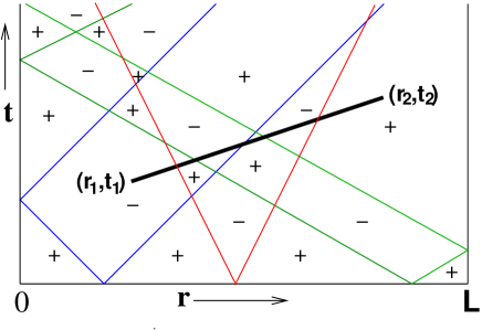
If a QP trajectory intersects the line $(r_{1},t_{1};r_{2},t_{2})$ an odd number of times, the spins at $(r_{1},t_{1})$ and $(r_{2},t_{2})$ have the opposite orientations (i.e. $\sigma_{r_{1}}^{x}(t_{1})=-\sigma_{r_{2}}^{x}(t_{2})$), which contributes to the decay of the correlation between $\sigma_{r_{1}}^{x}(t_{1})$ and $\sigma_{r_{2}}^{x}(t_{2})$, see Fig. 1. If the two trajectories pass an even number of times, the spins have the same orientation, as if the trajectories did not pass the line $(r_{1},t_{1};r_{2},t_{2})$ at all. Let $Q(r_{1},t_{1};r_{2},t_{2})$ be the probability, that the QPs, which have started from the same site, have passed the line $(r_{1},t_{1};r_{2},t_{2})$ a total odd number of times. Then the probability that for a given set of $n$ sites the kinks have passed (for each site total odd times) this line is: $Q^{n}(1-Q)^{L-n}$. Summing over all possibilities we have:

$$\dfrac{C(r_{1},t_{1};r_{2},t_{2})}{C_{\rm eq}(r_{1},r_{2})} = \sum_{n=0}^{L}(-1)^{n}Q^{n}(1-Q)^{L-n}\dfrac{L!}{n!(L-n)!}$$ (17)

$$= (1-2Q)^{L}\approx e^{-2Q(r_{1},t_{1};r_{2},t_{2})L}\;,$$

where $C_{\rm eq}(r_{1},r_{2})$ is the equilibrium correlation function in the initial state and in the last step we have used that the probability, $Q(r_{1},t_{1};r_{2},t_{2})$ is small. To calculate $Q$ one should average over the QPs with momenta $p\in[-\pi,\pi]$, or equivalently one can average over QP-pairs which is restricted to $p\in[0,\pi]$. In this second method we have the expression:

$$Q(r_{1},t_{1};r_{2},t_{2})=\frac{1}{2\pi}\int_{0}^{\pi}dp\;.f_{p}(h_{0},h)\cdot q_{p}(r_{1},t_{1};r_{2},t_{2})$$ (18)

in terms of the occupation probability (see Eq.(8)) and the passing probability, $q_{p}(r_{1},t_{1};r_{2},t_{2})$. This latter quantity measures the probability that the two trajectories $x_{1}(t)$ and $x_{2}(t)$ of any QP-pair with momentum $p$ intersect the line $(r_{1},t_{1};r_{2},t_{2})$ together an odd number of times. The same probability for a given QP-pair which is emitted at site $x_{0}\in[0,L]$ is denoted by $q_{p}(x_{0}|r_{1},t_{1};r_{2},t_{2})$. If we assume that the generation of QPs at the quench is homogeneous in space then we obtain:

$$q_{p}(r_{1},t_{1};r_{2},t_{2})=\dfrac{1}{L}\int_{0}^{L}dx_{0}\,q_{p}(x_{0}|r_{1},t_{1};r_{2},t_{2})\;.$$ (19)

In most cases of interest (see below) it is possible to provide an analytical form for the function $q_{p}(r_{1},t_{1};r_{2},t_{2})$. If not, the number of intersections can straightforwardly be determined numerically and averaged over $x_{0}$, yielding $q_{p}(r_{1},t_{1};r_{2},t_{2})$ and thus $Q(r_{1},t_{1};r_{2},t_{2})$ in Eq.(18) and the correlation function in Eq.(3).

IV Local magnetization

The time-dependent local magnetization at a site $l$ (here we consider $l\leq L/2$) can be formally expressed to a correlation between a spin that is fixed at time $t=0$ (to, say, $\sigma^{x}_{l}=+1$) and the same spin at later times $t$, i.e. $m_{l}(t)=m_{l}^{\rm eq}\cdot C|_{\sigma_{l}^{x}(t=0)=+}(l,0;l,t)$. Then, with Eq.(3)

$$m_{l}(t)=m_{l}^{\rm eq}\cdot e^{-2q(t,l)L}$$ (20)

with $q(t,l)=Q|_{\sigma_{l}^{x}(t=0)=+1}(l,0;l,t)$, which is with Eq.(18)

$$q(t,l)=\frac{1}{2\pi}\int_{0}^{\pi}dp\;f_{p}(h_{0},h)\,q_{p}(t,l)$$ (21)

where

$$q_{p}(t,l)=\dfrac{1}{L}\int_{0}^{L}dx_{0}\,q_{p}(x_{0},t,l)$$ (22)

as in Eq.(19). To calculate $q_{p}$ one concentrates first on times $t<T_{p}/2=L/2v_{p}$. Now $q_{p}$ is just the fraction of possible initial positions from which kink pairs can start with velocity $+v_{p}$ and $-v_{p}$ that flip the spin at position $l$ exactly once. This region is marked in the sketch of Fig. 2. One sees that for $t<l/v_{p}$ one gets $q_{p}=2vt/L$, and for $l/v_{p}<t<T_{p}/2$ one gets $q_{p}=2l/L$, independent of time.

Figure 2: Left: Typical semi-classical contribution to the time dependence of the local magnetization $m_{l}(t)$. Full lines are quasi-particles or kinks moving with velocity $v_{p}$ through the chain. The $\pm$ signs denote the sign of the spin at site $l$. Right: Sketch of the trajectories of kink pairs that flip the spin at position $l$ exactly once for times $t<T_{p}/2$. Kink pairs with initial position $x_{0}$ outside the marked region either do not flip the spin at $l$ (since they do not reach the position $l$ within time $t$) or they flip it twice. $q_{p}$ is the fraction of the marked intervals on the $t=0$-axis.

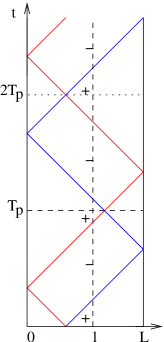
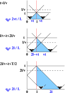
For $T_{p}/2<t<T_{p}$ one observes that a kink pair that started (at $t=0$) at position $x_{0}$ re-unites after a time $t=T_{p}$ at position $L-x_{0}$. Since the origins of kink pairs are distributed uniformly over the chain the probability $q_{p}(t,l)$ is $T_{p}$-periodic (n.b.: the kink trajectories themselves are only $2T_{p}$-periodic). Moreover $q_{p}(t,l)$ is symmetric with respect to time inversion since it is symmetric under the QP velocity inversion, $q_{p}(-t,l)=q_{p}(t,l)$, therefore $q_{p}(T_{p}-t,l)=q_{p}(t,l)$. Defining the reflection times $t_{1}=l/v_{p}$ and $t_{2}=T_{p}-t_{1}$ one then has for the period $0\leq t<T_{p}$ for $l<L/2$

$$q_{p}(t,l)=\left\{\begin{array}[]{lll}2v_{p}t/L&\quad{\rm for}&t\leq t_{1}\\ 2l/L&\quad{\rm for}&t_{1}\leq t\leq t_{2}\\ 2-2v_{p}t/L&\quad{\rm for}&t_{2}\leq t<T_{p}\end{array}\right.$$ (23)

For $l>L/2$ one uses the symmetry $q_{p}(t,l)=q_{p}(t,L-l)$ and for $t>T_{p}$ one makes use of the $T_{p}$-periodicity of $q_{p}(t,l)$:

$$q_{p}(t+nT_{p},l)=q_{p}(t,l),\quad(n=1,2,\ldots).$$ (24)

Although $q_{p}(t,l)$ is $T_{p}$-periodic, $q(t,l)$ is not periodic, since all QPs have different speed. Nevertheless the maximum speed $v_{\rm max}=h+{\cal O}(h^{2})$ determines the onset of magnetization reconstruction and therefore a quasi-periodicity of $q(t,l)$ and concomitantly $m_{l}(t)$, whose (quasi)-period is then expected to be

$$T_{\rm period}=L/v_{\rm max}\approx L/h$$ (25)

With Eqs.(21), (23) and (24) one obtains $m_{l}(t)$ via numerical integration (or summation over the discrete $p$-values for a lattice of finite size $L$).

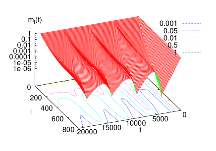
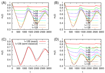
For an actual calculation one needs to know the occupation probability $f_{p}(h_{0},h)$ in Eq.(8), which can be calculated numerically in a straightforward manner using the free fermion technique. Since for large system sizes the occupation probability is not expected to depend strongly on the boundary condition we will use in the following the expression for $f_{p}(h_{0},h)$ for periodic boundary conditions, which can be given in analytical form as shown in Appendix A, see Eq.(60). In Fig. 3 the prediction of the semi-classical computation is shown. One observes the predicted quasi-periodicity for finite lattices and the expected exponential decays in $l$ and $t$ as discussed below.

Figure 3: Semi-classical prediction for the local magnetization $m_{l}(t)$ quench. Here $L=1024$, $h_{0}=0$, $h=0.2$. The (quasi)-periodicity (25) is $T_{\rm period}=L/h=5120$.

In Fig. 4 we compare the semi-classical prediction with the exact results obtained with the free fermion technique and find that the agreement is remarkably good. We observe that small deviations occur in the bulk ($l\sim L/2$) for $t>T_{\rm period}/2$, which is when the first QP reflections are involved in the dynamical evolution of $m_{l}(t)$. For sites close to the boundary, i.e. small $l$ we observe small deviations already in the plateau region (c.f. also the surface-to-bulk correlations discussed further below). Here a spatially inhomogeneous QP creation probabilities would have the most significant effect, which is negligible for bulk spins.

When the system after the quench would be thermalized at some effective temperature $T_{\rm eff}(h_{0},h)$ rossini this would imply that the occupation probability is

$$f_{p}(h_{0},h)=e^{-\epsilon_{p}(h)/T_{\rm eff}(h_{0},h)}\;.$$ (26)

The effective temperature is determined from the condition, that the relaxation time in equilibrium $\tau_{T}(h,T)$ (with transverse field $h$ and temperature $T$) is the same as in quantum relaxation at $T=0$ but after a quench from $h_{0}$ to $h$. In the limit $T\ll\Delta(h)$, $\Delta(h)$ being the gap of the system we havesachdev_young : $\tau_{T}(h,T)\approx\dfrac{\pi}{2T}e^{\Delta/T}$, which should be compared with $\tau(h_{0},h)$, which for small $h$ and $h_{0}$ is given in Eq.(44). The result of the semi-classical calculation using (26) is also shown in Fig. 4D and compared with the exact data for a quench form $h_{0}=0$ to $h=0.2$. One sees that, using the proper effective temperature the initial exponential decay agrees perfectly, but soon as the first reflections are involved, large deviations occur. An effective temperature can describe the initial relaxation well because essentially it is a fit parameter for the initial exponential decay, which stops after some ($l$-dependent) time in a finite system.

Figure 4: Relaxation of the local magnetization, $\log m_{l}(t)$, at different positions in a $L=256$ chain with free ends after a quench with parameters $h_{0}=0.0$, $h=0.2$ and $L=256$. A Exact (free fermion calculation). B Semi-classical prediction (20) with the passing probability (23) and the occupation probability (60). C Comparison between exact and QP calculation for $m_{l}(t)$ for $L=256$, $l=128$ for a quench from $h_{0}=0$ to $h=0.1$. D Semi-classical prediction using a thermal occupation number probability in Eq.(26) with an effective temperature, $T_{\rm eff}$, see the text.

In the infinite system size limit $L\to\infty$ the time $t_{2}$ in (23) is infinite for all momenta $p$. Thus the (quasi)-periodicity of $m_{l}(t)$ is lost and the functional form of $m_{l}(t)$ as predicted by (23), (21), and (20) is

$$m_{l}(t)= m_{l}^{\rm eq} \exp\left(-t\cdot\frac{2}{\pi}\int_{0}^{\pi}dp\,v_{p}\,f_{p}(h_{0},h)\,\theta(l-v_{p}t)\right)$$ (27)

$$\cdot \exp\left(-l\cdot\frac{2}{\pi}\int_{0}^{\pi}dp\,f_{p}(h_{0},h)\,\theta(v_{p}t-l)\right)$$

which defines, in analogy to sachdev_young the quench specific length and time scales

$$\tau_{\rm mag}^{-1}(h_{0},h) = \frac{2}{\pi}\int_{0}^{\pi}dp\,v_{p}\,f_{p}(h_{0},h)$$

$$\xi_{\rm mag}^{-1}(h_{0},h) = \frac{2}{\pi}\int_{0}^{\pi}dp\,f_{p}(h_{0},h)$$ (28)

In the small $h$ and $h_{0}$ limit these are calculated in Eqs.(44) and (37), respectively.

In a finite system there is a quasi-periodicity and the magnetization after the first relaxation period is reconstructed. Due to the $p$-dependence of the velocity of the QPs in the reconstruction regime the rate of exponential increase of the magnetization, $\tau^{\prime}_{\rm mag}$, is increasing in time. Its maximal value is reached at $t=T_{\rm period}$, which is given by:

$$\dfrac{1}{\tau^{\prime}_{\rm mag}(h_{0},h)} = \frac{2}{\pi}\left[\int_{\pi/6}^{\pi}-\int_{0}^{\pi/6}\right]dp\,v_{p}\,f_{p}(h_{0},h)$$ (29)

$$\approx h(h-h_{0})^{2}\dfrac{9\sqrt{3}-8}{12\pi}$$

where the second expression is valid in the small $h$ and $h_{0}$ limit. One can see that $\tau(h_{0},h)<\tau^{\prime}(h_{0},h)$, thus the reconstruction is slower than the relaxation. While QPs with large energy and high velocity contribute to the reconstruction, the other QPs with smaller energy and lower velocity still reduce the magnetization. These processes with opposite effect are responsible for the decay of the amplitude of the quasi-periodic oscillations of the profile, see Figs.3 and 4.

Figure 5: Relaxation of the local magnetization, $m_{l}(t)$ after quenches into the disordered phase – from the ordered phase ($h_{0}=0.5$, $h=1.5$) (A) exact, (B) semi-classical, and from the disordered phase ($h_{0}=1.5$, $h=2.0$) (C) exact, (D) semi-classical. The legend of A and B holds also for C and D, the system size is $L=256$.

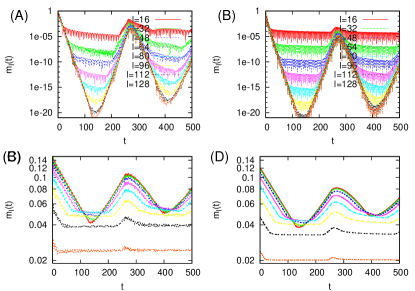
After quenches into the disordered phase ($h>1$) the relaxation (and recurrent) dynamics of the longitudinal magnetization is superposed by oscillations from the ground state correlations sachdev_young and one has to replace $m_{l}^{\rm eq}$ in (20) by

$$m_{l}^{\rm eq}\to m_{l}^{\rm eq}\cdot K(t\Delta)\;,$$ (30)

where $K(x)$ is the modified Bessel function. The results for the corresponding QP calculation and comparison with the exact data are shown in Fig. 5. One observes again that the relaxation and recurrent dynamics is well described by the semi-classical picture also for quenches into the paramagnetic (disordered) phase. The superposed oscillations have a slightly larger amplitude and frequency. Note also that for quenches from the paramagnetic phase (Fig. 5) C, D) the equilibrium profiles $m_{l}^{\rm eq})$ shifts the curves for $m_{l}(t)$ downwards for increasing $l$, since in the paramagnetic phase the surface magnetization is larger than the bulk magnetization in a finite chain (both vanishing only in the infinite system size limit).

V Correlation functions

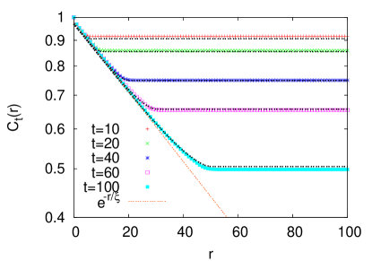
As mentioned before it is possible to perform the semi-classical calculation for the two-spin correlations $C(r_{1},t_{1};r_{2},t_{2})$ for any pair of sites $r_{1}$, $r_{2}$ and any pair of times $t_{1}$, $t_{2}$ with the formulas (3), (18), and (19). Here we want to focus on the time dependence of equal time correlations between spins separated by a distance $r$ and arranged symmetrically within the bulk, i.e. we consider

$$C_{t}(r)=C(L/2-r/2,t;L/2+r/2,t)\;,$$ (31)

for quenches within the ordered phase ($h<1$), which is, within the semi-classical theory given by:

$$C_{t}(r)=C_{\rm eq}(r)\cdot\exp\left(-\frac{\textstyle L}{\textstyle 2\pi}\int_{0}^{\pi}dp\;f_{p}(h_{0},h)\cdot q_{p}^{c}(t,r)\right)$$ (32)

Figure 6: (Color onlne) Semi-classical contributions to the equal time correlation function $C_{t}(r)=C(L/2-r/2,t;L/2+r/2,t)$. Left: Sketch of the trajectories of kink pairs that reverse the orientation of the spins at $r_{1}$ and $r_{2}$ for times $t<T_{p}/4$. Kink pairs with initial position $x_{0}$ outside the marked region either do not intersect the line $(r_{1}=L/2-r/2,t;r_{2}=L/2+r/2,t)$ (red) (since they do not reach the red line within the time $t$) or they flip it twice. $q^{c}_{p}$ is the fraction of the marked intervals on the $t=0$-axis. Right: Sketch of the additional symmetry of $q^{c}_{p}(t)$ that reduce its periodicity from $T_{p}$ to $T_{p}/2$: For each QP pair created at position $x_{0}$ intersection the red line at time $t<T_{p}/4$ there is a QP pair created at position $L-x_{0}$ that intersects the red line at time $T_{p}/2-t$. Hence $q^{c}_{p}(t)=q^{c}_{p}(T_{p}/2-t)$ for $t<T_{p}/2$. At $t=T_{p}/2$ the QP pair created at $x_{0}$ meets again at $L-x_{0}$ and the one created at $L-x_{0}$ meets again at $x_{0}$, which implies after averaging over initial position that $q^{c}_{p}(t+T_{p}/2)=q^{c}_{p}(t)$.

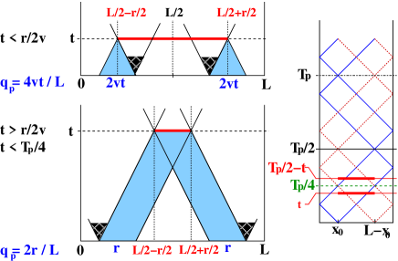
As sketched in Fig. 6 the function $q^{c}_{p}(r,t)$ for $C_{t}(r)$ is $T_{p}/2$-periodic and for the period $0\leq t<T_{p}/2$ given by for $r<L/2$

$$q^{c}_{p}(t,r)=\left\{\begin{array}[]{lll}4v_{p}t/L&\quad{\rm for}&t\leq t_{1}\\ 2r/L&\quad{\rm for}&t_{1}\leq t\leq t_{2}\\ 2-4v_{p}t/L&\quad{\rm for}&t_{2}\leq t<T_{p}/2\end{array}\right.$$ (33)

with $t_{1}=r/2v_{p}$ and $t_{2}=T_{p}/2-t_{1}$. (For $r>L/2$ one should replace in the above formulas $r$ to $L-r$.) Note that the relevant times occurring in this expression are all multiplied with a factor $1/2$ as compared to those determining $q_{p}$ for the local magnetization (23). In particular $q_{p}(t,r)$ is $T_{p}/2$-periodic (in contrast to the $T_{p}$ periodicity of $q_{p}$ for the local magnetization): $q_{p}(t+nT_{p}/2,r)=q_{p}(t,r)$ for $n=1,2,3,\ldots$. As a result the (quasi)-period of $C_{t}(r)$ for fixed $r$ is one half of the (quasi)-period of the local magnetization $m_{l}(t)$

$$T_{\rm period}^{C}=L/2v_{\rm max}\approx L/2h\;.$$ (34)

With (33) and $f_{p}(h_{0},h)$ from appendix A the semi-classical calculation can be performed, results and the comparison with exact data are shown in Fig. 7 and 8.

Figure 7: Equal time correlation function $C_{t}(r)$ for fixed $r$ as a function of time $t$ after the quench: Comparison between the exact result (left) and the semi-classical prediction (right). $L=256$, $h_{0}=0.$, $h=1.5$ (A) exact, (B) semi-classical; $h_{0}=0.3$, $h=0.5$ (C) exact, (D) semi-classical; The legend of A and B holds also for C and D.

Figure 8: Equal time correlation function $C_{t}(r)$ for fixed time $t$ after the quench as a function of distance $r$ Comparison between the exact result (points) and the QP calculation (black broken lines). $L=256$, $h_{0}=0$, and $h=0.25$.

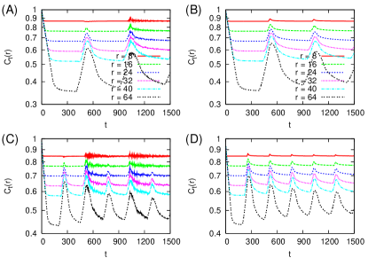
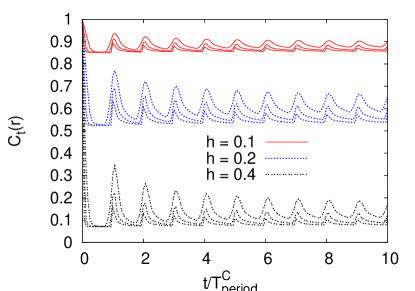
In 9 we show the semi-classical prediction for $C_{t}(r)$ for larger system sizes and long times, scaled by the (quasi)-period $T_{\rm period}^{C}$, (34), which demonstrates the persistence of the recurrence for very long times in finite systems. Note that the recurrence amplitude decreases with increasing system size and vanishes completely for $L\to\infty$.

Figure 9: QP prediction for the equal time correlation function $C_{t}(r)$ plotted against time after the quench scaled with the (quasi)-period $T_{\rm period}^{C}=L/2h$ for different fields $h$ ($h_{0}=0$). The three curves for each field $h$ correspond to different system sizes: $L=256$, $512$, and $1024$ (from the top curve to the bottom curve).

In the infinite system size limit $L\to\infty$ the time $t_{2}$ in (23) is infinite for all momenta $p$. Thus the (quasi)-periodicity of $C_{t}(r)$ is lost and the functional form of $C_{t}(r)$ as predicted by (33) and (32), is

$$C_{t}(r)= C_{\rm eq}(r) \exp\left(-t\cdot\frac{4}{\pi}\int_{0}^{\pi}dp\,v_{p}\,f_{p}\,\theta(l-v_{p}t)\right)$$ (35)

$$\cdot \exp\left(-r\cdot\frac{2}{\pi}\int_{0}^{\pi}dp\,f_{p}\,\theta(v_{p}t-l)\right)\;,$$

with $f_{p}=f_{p}(h_{0},h)$. This agrees to first order in $f_{p}$ to the prediction of Calabrese2 , where $f_{p}$ is replaced by $-1/2\;\log(1-2f_{p})=f_{p}+{\cal O}(f_{p}^{2})$ (see appendix A). Eq. (35) defines the quench specific length and time scales

$$\tau_{c}^{-1}(h_{0},h) = \frac{4}{\pi}\int_{0}^{\pi}dp\,v_{p}\;f_{p}(h_{0},h)$$

$$\xi_{c}^{-1}(h_{0},h) = \frac{2}{\pi}\int_{0}^{\pi}dp\,f_{p}(h_{0},h)$$ (36)

Note that $\tau_{c}=\tau_{\rm mag}/2$ and $\xi_{c}=\xi_{\rm mag}$. For a small $h_{0}$ and $h$ this yields to leading order

$$\xi^{-1}(h_{0},h)=\dfrac{(h-h_{0})^{2}}{2\pi}\int_{0}^{\pi}{\rm d}k\sin^{2}k=\dfrac{(h-h_{0})^{2}}{4}$$ (37)

V.1 Surface-to-bulk correlation

The surface-to-bulk correlation function $C_{t}^{\rm surf}(r)=C(0,t;r,t)$ is within semi-classical theory given by

$$C_{t}^{\rm surf}(r)=C_{\rm eq}^{\rm surf}(r)\cdot\exp\left(-\frac{\textstyle L}{\textstyle\pi}\int_{0}^{\pi}dp\,f_{p}\cdot q^{\rm surf}_{p}(t,r)\right)$$ (38)

with $f_{p}=f_{p}(h_{0},h)$. Similar considerations that lead to (23) and (33) yield an analytical expression for $q_{p}^{\rm surf}(t,r)$, which is equivalent to $q_{p}(t,l)$ for the local magnetization in (23), however with $l=r$:

$$q_{p}^{\rm surf}(t,r)=q_{p}(t,l=r)\;.$$ (39)

Consequently

$$C_{t}^{\rm surf}(r)=C_{\rm eq}^{\rm surf}(r)\frac{m_{l=r}(t)}{m_{l=r}^{\rm eq}}\;.$$ (40)

which implies that the surface-bulk correlation is dominated by the relaxation of the magnetization at the bulk site and that it is $T_{p}$-periodic (in contrast to $C_{t}(r)$, which is $T_{p}/2$-periodic.

In Fig. 10 we show a comparison of this semi-classical result with the exact data. We observe that small deviations occur in the plateau region for small distances $r$ where the bulk-correlations still agree very well with the semi-classical prediction. Since for small $r$ both sites in the surface-to-bulk correlation function are close to the boundary a spatially inhomogeneous QP creation probabilities would have the most significant effects here.

Figure 10: Surface-to-bulk correlation function $C_{t}^{\rm surf}(r)$ for fixed time $r$ as a function of the time after the quench. Comparison between the exact result (points) and the QP calculation (black broken lines). $L=256$, $h_{0}=0.75$, and $h=0.25$.

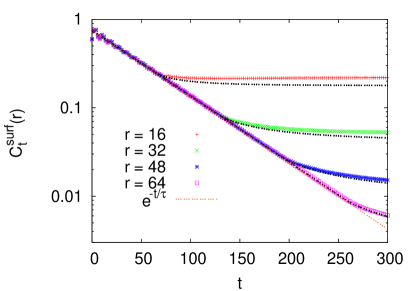
V.2 Autocorrelations

The autocorrelation function

$$G_{l}(t)=C(l,0;l,t)$$ (41)

is (up to an extra factor $m_{l}^{\rm eq}$) identical to the time-dependent local magnetization $m_{l}(t)$:

$$G_{l}(t)=G_{\rm eq}\frac{m_{l}(t)}{m_{l}^{\rm eq}}\;.$$ (42)

For $l=L/2$ (bulk autocorrelation) in the limit $L\to\infty$ the QP prediction is

$$G_{L/2}(t) \propto \exp\left(-\frac{2}{\pi}\int_{0}^{\pi}dp\;f_{p}(h_{0},h)\cdot v_{p}t\right)$$ (43)

$$= e^{-t/\tau_{\rm auto}}$$

with the relaxation time $\tau_{\rm auto}=\tau_{\rm mag}$, eq.(28), which corresponds to the leading order of the result from Calabrese et al Calabrese2 (see appendix A), in which $f_{p}$ is again replaced by $-1/2\;\log(1-2f_{p})=f_{p}+{\cal O}(f_{p}^{2})$. For a small $h_{0}$ and $h$ (28) yields to leading order

$$\tau^{-1}=\dfrac{h(h-h_{0})^{2}}{2\pi}\int_{0}^{\pi}{\rm d}k\sin^{3}k=h(h-h_{0})^{2}\dfrac{2}{3\pi}\;.$$ (44)

This has already been found numerically inigloi_rieger2 .

VI Periodic boundary conditions

In a chain with periodic boundary conditions instead of the open boundaries that we considered so far, one has to replace the QP trajectories (16) by the appropriate expressions:

$$x_{1}(t)=(x_{0}+v_{p}t)\;{\rm mod}\;L$$

$$x_{2}(t)=(x_{0}-v_{p}t)\;{\rm mod}\;L$$ (45)

where the modulo operation is defined in the obvious manner: Shift the real number $x_{i}$ by multiples of $L$ such that it lays in the interval $[0,L]$. With this the evaluation of the local magnetization and correlation functions is straight-forward.

The chain with periodic boundary conditions is translationally invariant, therefore the equal time correlation $C_{t}^{\rm p.b.c.}(r)=C^{\rm p.b.c.}(r_{1},t_{1};r_{1}+r,t_{2})$ is independent of $r_{1}$. One sees immediately that the expression for $q_{p}^{\rm p.b.c.}(t,r)$ is identical to $q_{p}^{c}(t,r)$ in Eq. (33), and therefore $C_{t}^{\rm p.b.c}(r)$ is identical, up to prefactors from the ground state or equilibrium correlation function, to $C^{\rm open}(L/2-r/2,t;L/2+r/2,t)$:

$$C_{t}^{\rm p.b.c.}(r)=\frac{C_{\rm eq}^{\rm p.b.c.}(r)}{C_{\rm eq}^{\rm open}(r)}\cdot C_{t}^{\rm open}(r)$$ (46)

It should be noted that this relation only holds for the symmetric correlation function $C_{t}^{\rm open}(r)=C^{\rm open}(L/2-r/2,t;L/2+r/2,t)$.

The local magnetization $m_{l}(t)$ is independent of the site $l$ in a system with periodic boundary conditions, as is the QP passing probability $q_{p}^{\rm p.b.c.}(t,l)=q_{p}^{\rm p.b.c.}(t)$. We find

$$q_{p}^{\rm p.b.c.}(t)=\left\{\begin{array}[]{lll}2v_{p}t/L&\quad{\rm for}&t\leq T_{p}/2\\ 2-2v_{p}t/L&\quad{\rm for}&T_{p}/2<t\leq T_{p}\end{array}\right.$$ (47)

For $t>T_{p}$ one uses the $T_{p}$-periodicity $q_{p}^{\rm p.b.c.}(t+nT_{p})=q_{p}^{\rm p.b.c.}(t)$, $(n=1,2,\ldots)$. With eq. (20) and (21) the local magnetization is then given by

$$\frac{m^{\rm p.b.c.}(t)}{m_{\rm eq}^{\rm p.b.c.}}=\exp\left(-\frac{2}{\pi}\int_{0}^{\pi}dp\;f_{p}\,v_{p}t\,\theta(\sin(2\pi t/T_{p}))\right.$$

$$\left.\qquad+\frac{2}{\pi}\int_{0}^{\pi}dp\;f_{p}\,(L-v_{p}t)\,\theta(-\sin(2\pi t/T_{p}))\right)$$ (48)

In the infinite system size limit this yields

$$m^{\rm p.b.c.}(t)\propto\exp\left(-t\frac{2}{\pi}\int_{0}^{\pi}dp\;f_{p}\,v_{p}\right)\propto e^{-t/\tau_{\rm mag}}\;,$$ (49)

which agrees to first order in $f_{p}$ with the prediction of Calabrese2 . As for open boundary conditions the autoscorrelation function $G^{\rm p.b.c.}(t)$ is given, up to prefactors, by the same expression as the local magnetization (48).

VII Discussion

We have formulated a semi-classical theory for the non-equilibrium quantum relaxation of the transverse Ising chain after a global quench via an instantaneous change of the transverse field. It is applicable to systems of finite and infinite length and describes properly the relaxation dynamics as well as the recurrence / reconstruction properties of dynamical correlations in finite systems. For infinite systems our theory agrees to lowest order with a recent prediction by Calabrese et alCalabrese2 . Our results indicate that the global quantum quench induces a unique length-scale, $\xi$, and a unique time-scale, $\tau$, in the system, both dependent upon the quench parameters, $h_{0}$ and $h$. These characteristic scales appear also in half-infinite geometry and in finite systems, provided the length of the system is larger than $\xi$. In a finite system this semi-classical theory not only explains the recurrence and reconstruction properties of the local magnetizationigloi_rieger2 , but describes the dynamical behavior quantitatively.

The semi-classical theory can be used to define an effective temperature for the quantum relaxation process. If we compare the expressions obtained by Sachdev and Youngsachdev_young for the correlation length and the relaxation time in equilibrium at finite temperatures with our results for zero temperature quantum quenches one obtains a node-dependent effective temperature, $T_{\rm eff}(p)$, defined by the condition:

$$f_{p}(h_{0},h)=\exp\left(-\dfrac{\varepsilon_{h}(p)}{T_{\rm eff}(p)}\right)\;.$$ (50)

This relation agrees to first order in $f_{p}$ with the prediction of Calabrese2 (i.e. for small effective temperatures or small differences $|h-h_{0}|$). In Calabrese2 the Boltzmann-factor on the r.h.s. of Eq.(50) is replaced by the Fermi-function with zero chemical potential, as shown in the Appendix in Eq.(63), thus replacing classical kinks simply by free fermions.

It is interesting to notice an analogous expression for the time-evolution of the entanglement entropy, $S(t)$, measured after the quench between two semi-infinite parts of the system, say ${\cal A}$ and ${\cal B}$. The analytical result by Fagotti and Calabresefagotti_calabrese can be written into the form:

$$S(t)=t\frac{1}{\pi}\int_{0}^{\pi}dp\,v_{p}\,s_{p}(h,h_{0})\;,$$ (51)

with

$$s_{p}(h,h_{0})=-(1-f_{p})\ln(1-f_{p})-f_{p}\ln f_{p}\;,$$ (52)

being the entropy of the fermionic mode with occupation number $f_{p}(h_{0},h)$. In the semi-classical theory this expression can be interpreted as the result of ballistically moving QP pairs, which are created say at ${\cal A}$ at $t=0$ and one of them is reaching ${\cal B}$ before the actual time, $t$. Each of these QPs brings an entropic contribution as a free fermion. It would be interesting to see if the relations in Eqs.(63) and (51) are valid for another integrable quantum spin systems, too.

The semi-classical approach is accurate, if the occupation probability, $f_{p}(h_{0},h)$, is small, which is valid if the initial and the finite states are close to each other and both are ferromagnetic. As shown inigloi_rieger2 for $h,h_{0}<1$ the magnetization profile $m_{l}(t)$ for any finite $l$ and $t$ is non-negative. In the other domains of the quench ($h_{0}$ and/or $h$ is larger than $1$) during relaxation $m_{l}(t)$ takes negative values, too. This type of oscillating relaxation is described qualitatively well by the semi-classical theory. The amplitude of the oscillations as well as the recurrence of the magnetization and the correlations are correctly described, but there are differences in the actual value of the frequencies. For quenches close to the critical point we expect the concept of isolated QPs to become invalid or at least quantitatively inaccurate due to the diverging correlation length either in the initial and / or final state.

In finite system with open boundaries and for half-infinite systems we find small deviations between the exact and the semi-classical results either when sites close to the boundaries are involved or for times $t>T_{\rm period}/2$, when QPs reflected at the boundaries contribute to the magnetization or correlation reconstruction. A possible source for the deviations in the first case is the lack of translational invariance in chains with open boundaries, which results in spatially inhomogeneous creation probability of QP pairs, at least close to the boundaries. The second kind of deviations could originate in the dynamical processes during the reflection at the open boundaries, which might be more complicated than just momentum inversion. Both effects are absent in systems with open boundaries, for which reason we expect our predictions to be accurate for all times in finite chains with periodic boundary conditions.

Our semi-classical theory can be generalized to several directions. This theory is also valid for transverse Ising chains involving a sum over more ferromagnetic short-range interactions than only nearest neighbors, as has been argued for the equilibrium relaxation dynamics at finite temperatures by Sachdev and Youngsachdev_young . The semi-classical theory should be applicable to non-integrable models, too, for which one has to include QP-collision and scattering processes. Here the quantum Boltzmann equation seems to be a promising approach ziman , as has been demonstrated recently for a bosonic system in rosch .

Appendix

Here we compare our semi-classical calculation with the predictions by Calabrese et alCalabrese2 . First we recapitulate the exact solution of the free fermion representation the Hamiltonian in Eq.(4) for periodic boundary conditions. In this case there are pairs of fermions with quasi-momenta $p$ and $-p$, and in the ground state sector these are: $p=\dfrac{\pi}{L},\dfrac{3\pi}{L},\dfrac{5\pi}{L},\dots$, $0<p<\pi$. Here we define the functions:

$$u_{h}(p) = \sqrt{\dfrac{\varepsilon_{h}(p)+h-\cos p}{2\varepsilon_{h}(p)}}$$

$$v_{h}(p) = \sqrt{\dfrac{\varepsilon_{h}(p)-(h-\cos p)}{2\varepsilon_{h}(p)}}$$ (53)

and

$$U_{p}=u_{h_{0}}(p)u_{h}(p)+v_{h_{0}}(p)v_{h}(p)$$ (54)

$$V_{p}=u_{h_{0}}(p)v_{h}(p)-v_{h_{0}}(p)u_{h}(p)$$ (55)

in terms of which the ground state for $t<0$ ($|\Psi_{0}\rangle$) is expressed with the ground state at $t>0$ ($|0\rangle$) as:

$$|\Psi_{0}\rangle=\prod_{p}\left[U_{p}+iV_{p}\eta_{p}^{{\dagger}}\eta_{-p}^{{\dagger}}\right]|0\rangle$$ (56)

Then the density of quasi-particle excitations is given by the nonequilibrium occupation number:

$$f_{p}=\langle\Psi_{0}|\eta_{p}^{{\dagger}}\eta_{p}|\Psi_{0}\rangle=|V_{p}|^{2}$$ (57)

This can be expressed as:

$$f_{p}=\dfrac{1}{2}\left[1-\cos\Delta_{p}\right]$$ (58)

where $\Delta_{p}$ is the difference between the Bogoliubov angles diagonalizing ${\cal H}(h)$ and ${\cal H}(h_{0})$, respectively:

$$\cos\Delta_{p}=\dfrac{h_{0}h-(h_{0}+h)\cos p+1}{\varepsilon_{h_{0}}(p)\varepsilon_{h}(p)}$$ (59)

If the difference between $h_{0}$ and $h$ is small we obtain in leading order for the occupation number:

$$f_{p}=\dfrac{1}{4}(h-h_{0})^{2}\sin^{2}p$$ (60)

The results by Calabrese et alCalabrese2 can be formally obtained from our semi-classical expressions, if an effective occupation number is used. For example in Eq.(37) for the correlation length and in Eq.(44) for the relaxation time one should simply replace:

$$f_{p}\to-\dfrac{1}{2}\ln|\cos\Delta_{p}|$$ (61)

The semi-classical results then represent the leading term of the exact expressions.

According to Calabrese et alCalabrese2 there is an effective thermal (Gibbs) distribution or generalized Gibbs ensemble (GGE), which is obtained in integrable models by maximizing the entropy, while keeping the energy and other conservation laws fixed. This leads to an effective, node-dependent temperature: $T_{\rm eff}(p)$, which is given by:

$$\cos\Delta_{p}=\tanh\dfrac{\epsilon_{h}(p)}{2T_{\rm eff}(p)}\;,$$ (62)

or expressed with $f_{p}$ we have:

$$f_{p}=\dfrac{1}{\exp\left(\dfrac{\varepsilon_{h}(p)}{T_{\rm eff}(p)}\right)+1}.$$ (63)

At the r.h.s. we have the Fermi distribution function with zero chemical potential, thus the GGE condition is expressed in the form, that the nonequilibrium occupation number of the given mode is equal to its thermal occupation at the effective temperature: $T_{\rm eff}(p)$.