Many-Body Effects in a Model of Electromagnetically Induced Transparency

Abstract

We study the spectral properties of a many-body system under a regime of electromagnetically induced transparency. A semi-classical model is proposed to incorporate the effect of inter-band interactions on an otherwise single-body scheme. We use a Hamiltonian with non-Hermitian terms to account for the effect of particle decay from excited levels. We explore the system response as a result of varying the interaction parameter. Then we focus on the highly interacting case, also known as the blockade regime. In this latter case we present a perturbative development that allows to get the transmission profile for a wide range of values of the system parameters. We observe a reduction of transmission when interaction increases and show how this property is linked to the generation of a strongly correlated many-body state. We study the characteristics of such a state and explore the mechanisms giving rise to various interesting features.

The study of light–matter interaction has experienced a pronounced development over the last few decades, both experimentally and theoretically. In this process, progress has been made by advancing the foundations laid by pioneering observations, such as electromagnetically induced transparency (EIT), stimulated Raman adiabatic passage (STIRAP) and coherent population trapping (CPT). Such techniques can be understood in terms of single particle models, making it possible to obtain much insight into the physical background leading to the realisation of the mentioned phenomena. Similarly, due to the increasing level of control possible in low-temperature physics, the transition toward more collectively driven scenarios is starting to attract general attention.

Figure 1: Diagram of EIT including several particles. The dynamics is determined by the coupling and probe lasers which drive particles between the ground and excited bands and the excited and interaction (Rydberg) bands respectively. In addition, the first excitation levels of a system with 8 bosons are shown.

One way of understanding the mechanism underlying EIT is to think in terms of cancellation of excitation pathways with opposite phases [1]. As the process involving the absorption of one photon is on-resonance, a different transition enhancing photon emission arises with equal intensity and opposite phase. The result can then be seen as pure quantum interference. An alternative way is to view the optical field as interacting with just one of two possible coupling modes [2]. The resonant mode is related to the so-called dark state, which displays a decay time much lower than other possible configurations, which allows for the whole system to be pumped into this dark state by the combined action of probe and coupling lasers. These views are useful when many-body effects are taken into consideration, but signatures of collective behaviour slowly degrade the single particle response [3], and a more detailed analysis becomes necessary. This response results as a consequence of the interaction among particles and is an instance in which photons communicate using matter as an intermediary [4]. In this direction, an interesting problem is the study of the many-body physics behind the interference mechanism governing EIT. An example of this is the realisation of clean EIT-profiles on ensembles of interacting atoms [5, 6].

Atoms with very high principal quantum number—also known as Rydberg atoms–display important properties that make them useful in several applications. In particular, the interaction among Rydberg atoms gives rise to a blockade mechanism originated by dipole–dipole interactions or van der Waals forces. The blockade process can be exploited in diverse applications, such as quantum gates proposals [10, 11, 8, 7, 9], cavity QED constructs [12, 13], the generation of entanglement [14, 15, 16], adiabatic passage [17, 18] and numerous quantum information techniques [19].

For the specific case of EIT, inter-atomic interactions produce a highly robust state with a collective character. As discussed in reference [5], the quantum superposition can be seen as involving states where due to dipole–dipole interactions only a single atom can be excited to the interacting band and therefore only one atom is involved in EIT. This results in a reduction of transparency as the possibilities of interference of excitation pathways are diminished. Such reduction shows neither resonance-shift nor line-width broadening. Some of the experimental results cannot be explained via mean-field approximations and full quantum models must be employed to reproduce the observed features [6]. In reference [20] it was shown that two-photon correlations lead to an enhanced attenuation of the probe beam for strong intensities and in this way a detailed description of the experiment in reference [5] is achieved. When emphasis is made on the propagation of the probe laser through the medium as in [21], it is shown that the blockade mechanism gives rise to a highly non-local response in addition to non-linearities.

Many-body effects in an ensemble of interacting atoms can be studied using the master equation formalism [22]. In this case the number of coefficients necessary to describe the density matrix is proportional to the square of the total number of elements in the Hilbert space. Instead, we probe the advantages of introducing decay factors as imaginary elements in the Hamiltonian, so that the whole analysis can be carried in terms of state functions, providing insight into the development of the many-body scenario as well as the statistical effects that arise due to the bosonic nature of the particles. Non-Hermitian Hamiltonians (NHH) have proved useful in several studies, e.g., single particle models of EIT [1], STIRAP in the presence of degenerate product states [23, 24] and the dynamics of Bose–Hubbard dimers [25] among many others. This approach is reasonable since we want to explore the case of high number of particles where standard approximations have displayed mixed results [26]. Below we show that the proposed methodology produce consistent results and is especially suitable to develop a perturbative approach which is valid over a wide range of parameters. The insight acquired in this way is less accessible using a fully numerical approach since several tunable parameters must be considered.

In our proposal we assume that probe and coupling lasers induce particle exchange among three energy levels as in a ladder EIT scheme [5, 17] (figure 1) and that two-body interactions take place only in the interaction band. Such two-body exchange is mediated by a constant parameter $U$. In general, the interaction depends on the inter-atomic distance and the Rydberg principal quantum number [5, 19]. Using a semi-classical approach and incorporating the rotating wave approximation in addition to non-Hermitian decay-terms the NHH reads,

$$\hat{H}=-\Omega_{c}e^{-i\omega_{c}t}\hat{a}_{R}^{\dagger}\hat{a}_{e}-\Omega_{p}e^{-i\omega_{p}t}\hat{a}_{g}^{\dagger}\hat{a}_{e}+H.c.$$

$$+\frac{U}{2}\hat{a}_{R}^{\dagger}\hat{a}_{R}(\hat{a}_{R}^{\dagger}\hat{a}_{R}-1)-i\Gamma_{R}\hat{a}_{R}^{\dagger}\hat{a}_{R}-i\Gamma_{e}\hat{a}_{e}^{\dagger}\hat{a}_{e}$$

$$+E_{g}\hat{a}_{g}^{\dagger}\hat{a}_{g}+E_{R}\hat{a}_{R}^{\dagger}\hat{a}_{R}+E_{e}\hat{a}_{e}^{\dagger}\hat{a}_{e}.$$ (1)

Creation and annihilation operators introduce boson-like statistics through the commutation relations $[\hat{a}_{L},\hat{a}_{L}^{\dagger}]=1$ for $L=g,e,R$. $\Omega_{p}$ and $\Omega_{c}$ are the probe- and coupling-Rabi frequencies respectively. Similarly, $\omega_{p}$ and $\omega_{c}$ are the laser frequencies while $E_{g}$, $E_{R}$ and $E_{e}$ represent the energies of the corresponding bands. The intensity of particle decay from the interaction- and excited-bands is controlled via $\Gamma_{R}$ and $\Gamma_{e}$ respectively. Both constants are positive definite. This approach is valid in the limit of weak coupling between the ground and excited bands [1]. In our analysis we set $\hbar=1$ and measure all the parameters in recoil energies $E_{r}=\hbar^{2}K^{2}/(2m)$. The energy structure of the system correspond to three-level EIT-picture where $E_{R}>E_{e}>E_{g}$ (figure 1). Although not explicit in (1), the total number of particles is $M$, which accounts for the number of atoms in a blockade sphere. The proposed scheme can be realised by projecting counter-propagating lasers onto a cloud of ultra-cold atoms—for example, ⁸⁷Rb. These lasers provide the probe- and coupling-frequencies in our proposal. The number of atoms can be controlled by pumping atoms into energy levels that do not couple to the probe- or coupling-lasers. The energy spectrum of the gas contains bands that can stand for the ground and excited bands of figure 1. The gas also contains highly excited atoms which display interaction intensities much larger than atoms in the ground or excited levels, so that it is valid to neglect interaction effects on these bands. The intensity of the interaction can be tuned using Feshbach resonance [27]. Actual experiments implementing this approach have been reported in several works, as for instance in references [5, 6]. As a result of the inclusion of non-Hermitian terms in equation (1), the wave function norm is no longer preserved and therefore the quantum state must be normalised in anticipation to any explicit calculation. After an appropriate transformation we get the following dressed NHH in the interaction picture,

$$\hat{H}_{D}=-\Omega_{c}(\hat{a}_{R}^{\dagger}\hat{a}_{e}+\hat{a}_{e}^{\dagger}\hat{a}_{R})-\Omega_{p}(\hat{a}_{g}^{\dagger}\hat{a}_{e}+\hat{a}_{e}^{\dagger}\hat{a}_{g})$$

$$+\frac{U}{2}\hat{a}_{R}^{\dagger}\hat{a}_{R}(\hat{a}_{R}^{\dagger}\hat{a}_{R}-1)-i\Gamma_{R}\hat{a}_{R}^{\dagger}\hat{a}_{R}-i\Gamma_{e}\hat{a}_{e}^{\dagger}\hat{a}_{e}$$

$$+\delta\hat{a}_{g}^{\dagger}\hat{a}_{g}+(E_{R}-\omega_{c})\hat{a}_{R}^{\dagger}\hat{a}_{R}+E_{e}\hat{a}_{e}^{\dagger}\hat{a}_{e},$$ (2)

where $\delta=E_{g}-\omega_{p}$. For simplicity we have assumed single photon resonance and without loss of generality we set $E_{R}-\omega_{c}=E_{e}=0$. Here we are mainly concerned with the magnitude of the coupling between the atoms and the probe laser, i.e., the atomic susceptibility. Hence we focus on the mean value,

$$\chi_{M}^{(n)}=\frac{\langle\left(\hat{a}_{g}^{\dagger}\hat{a}_{e}\right)^{n}\rangle}{M^{n}}.$$ (3)

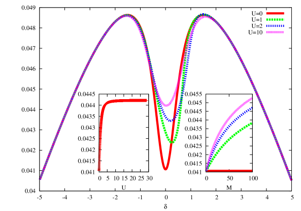
Figure 2: $\chi_{M}^{(1)}$ for $M=50$, $\Gamma_{e}=10$, $\Gamma_{R}=0.5$, $\Omega_{c}=1$, $\Omega_{p}=0.5$. Inset: Same parameters and $\delta=0$. Left: $\chi_{M}^{(1)}$ against $U$. Right:$\chi_{M}^{(1)}$ against $M$. The large dip in the main figure features a decrease of absorption of the probe laser at zero detuning. Increasing the interaction provokes a reduction of transmission. As shown in the insets, this effect can be controlled by tuning either the intensity of the interaction or the number of particles.

Imaginary and real parts of $\chi_{M}^{n}$ account for different orders of absorption and refraction respectively. Figure 2 presents the behaviour of $\chi_{M}^{(1)}$ as various parameters are tuned. In all cases the state of the system is given by the right eigenstate of equation (2) corresponding to the eigenvalue with the highest imaginary part (the less decaying state). The NHH (2) conserves the total number of particles so that the full dimension of the Hilbert space is $(M+2)(M+1)/2$. The pattern shown in figure 2 is proportional to the transmission profile of the probe laser. It indicates a characteristic window of transparency that results from the combined action of the incident lasers. In the absence of interaction the dip in absorption can be ascribed to interference of pathways with opposite phases, i.e., the process by which one atom goes from $|g\rangle$ to $|e\rangle$ is cancelled out by the process by which the atom goes from $|e\rangle$ to $|R\rangle$ and then all the way back from $|R\rangle$ to $|e\rangle$ to $|g\rangle$ again. As can be seen, the case $U=0$, which is equivalent to the single particle case, displays the maximum interference. As the interaction is gradually turned on, the two-photon resonance is shifted to the right due to the energy increase of the interaction band produced by the repulsion among particles. $\chi_{M}$ continues to grow until it reaches a saturation value, but without completely suppressing transparency. $\chi_{M}$ also grows with $M$, but no saturation is visible over values of $M$ less than 100. In general, we can see that the insertion of particles causes a reduction of quantum interference. Such an effect can be enhanced either by increasing $U$ or $M$. However, in every case the physical response is different. While changing $U$ affects the intensity of two-body interactions, adding particles produces a (sometimes steep) rearrangement of the quantum state.

From the Heisenberg equations we can extract the expression,

$$\frac{d\hat{\alpha}_{g}^{\dagger}}{dt}=i\Omega_{p}\hat{\alpha}_{e}^{\dagger}-i\delta\hat{\alpha}_{g}^{\dagger},$$ (4)

where $\hat{\alpha}_{n}^{\dagger}=e^{-it\hat{H}_{D}}\hat{a}_{n}^{\dagger}e^{it\hat{H}_{D}}$ for $n=g,R,e$. Since $\Omega_{p}<<\Omega_{c}$ we can assume that $\hat{\alpha}_{g}^{\dagger}$ does not greatly influence the evolution of $\hat{\alpha}_{R}^{\dagger}$ and $\hat{\alpha}_{e}^{\dagger}$, so that $\hat{\alpha}_{e}^{\dagger}$ can be treated as a function of time. Thus it follows that,

$$\hat{\alpha}_{g}^{\dagger}(t)=i\Omega_{p}e^{-i\delta t}\int_{0}^{t}e^{i\delta T}\hat{\alpha}_{e}^{\dagger}(T)dT.$$ (5)

Under such an assumption, in the blockade regime equation (2) can be reduced to a Jaynes–Cummings-like Hamiltonian on the interaction- and excited-bands,

$$\hat{H}_{Re}=-\Omega_{c}(\hat{\sigma}^{+}\hat{a}_{e}+\hat{\sigma}^{-}\hat{a}_{e}^{\dagger})-i\Gamma_{R}\left(\frac{\hat{\sigma}_{z}+1}{2}\right)-i\Gamma_{e}\hat{a}_{e}^{\dagger}\hat{a}_{e},$$ (6)

where we have employed Pauli matrices to account for the dynamics of the interaction band. The eigensystem of equation (6) is given by [28],

$$E=0,\hskip 14.22636pt|0,0\rangle,\hskip 14.22636pt\langle 0,0|,$$ (7)

$$E_{n}^{\pm}=-i(\Gamma_{e}n+\Gamma_{R}+\Omega_{c}\sqrt{n+1}e^{\pm i\theta_{n}}),$$ (8)

$$|E_{n}^{\pm}\rangle=(|1,n\rangle+ie^{\pm i\theta_{n}}|0,n+1\rangle)/Z_{n}^{\pm},$$ (9)

$$\langle E_{n}^{\pm}|=(\langle 1,n|+ie^{\pm i\theta_{n}}\langle 0,n+1|)/Z_{n}^{\pm},$$ (10)

where,

$$Z_{n}^{\pm}=\sqrt{1-e^{\pm 2i\theta_{n}}},$$ (11)

$$\cos\theta_{n}=\frac{\Gamma_{e}-\Gamma_{R}}{2\Omega_{c}\sqrt{n+1}},\hskip 5.69046ptn=0,1,\dots,M-1.$$ (12)

The first and second integers in a ket (bra) correspond to the number of particles in the interaction (excited) band. The angle $\theta_{n}$ is complex as well as the eigenvalues of the NHH. In the form in which they appear above, the eigenvectors satisfy $\langle E_{k}^{s}|E_{k^{\prime}}^{s^{\prime}}\rangle=\delta_{k}^{k^{\prime}}\delta_{s}^{s^{\prime}}$. This eigensystem can be used to write,

$$\hat{H}_{Re}=\sum_{n=0}^{M-1}E_{n}^{\pm}|E_{n}^{\pm}\rangle\langle E_{n}^{\pm}|.$$ (13)

The spectrum of the NHH is well defined except when $\cos\theta_{n}=1$, in which case the eigenvectors (9) and (10) become indeterminate but one can still recover the NHH as the limit of equation (13). These singularities therefore produce removable discontinuities leading to no divergence in the mean values of the system’s observables. Now we project on the subspace associated to the NHH,

$$\hat{a}_{e}^{\dagger}=\hat{a}_{e}^{\dagger}\left\{\sum_{n=0}^{M-1}|E_{n}^{\pm}\rangle\langle E_{n}^{\pm}|+|0,0\rangle\langle 0,0|\right\}.$$ (14)

This procedure is facilitated by introducing the coefficients validating the following identities:

$$\hat{a}_{e}^{\dagger}|0,0\rangle=c_{0}^{+}|E_{0}^{+}\rangle+c_{0}^{-}|E_{0}^{-}\rangle,$$ (15)

$$\hat{a}_{e}^{\dagger}|E_{n}^{+}\rangle=c_{n+1}^{+}|E_{n+1}^{+}\rangle+c_{n+1}^{-}|E_{n+1}^{-}\rangle,$$ (16)

$$\hat{a}_{e}^{\dagger}|E_{n}^{-}\rangle=d_{n+1}^{+}|E_{n+1}^{+}\rangle+d_{n+1}^{-}|E_{n+1}^{-}\rangle.$$ (17)

Once $\hat{a}_{e}^{\dagger}$ is written in terms of the eigenvectors of the NHH we can calculate $\hat{\alpha}_{e}^{\dagger}$ and replace it in equation (5) where we can now carry on the integration in terms of time. The result can be written in the form,

$$\hat{\alpha}_{g}^{\dagger}(t)=\hat{a}_{g}^{\dagger}+\Omega_{p}\left(\hat{\kappa}(0)-e^{-i\delta t}\hat{\kappa}(t)\right),$$ (18)

where,

$$\hat{\kappa}(t)=\frac{c_{0}^{+}e^{-it(E_{0}^{+}-\delta)}|E_{0}^{+}\rangle\langle 0,0|}{E_{0}^{+}-\delta}+\frac{c_{0}^{-}e^{-it(E_{0}^{-}-\delta)}|E_{0}^{-}\rangle\langle 0,0|}{E_{0}^{-}-\delta}+$$

$$\sum_{n=0}^{M-2}\left(\frac{c_{n+1}^{+}e^{-it(E_{n+1}^{+}-E_{n}^{+}-\delta)}|E_{n+1}^{+}\rangle\langle E_{n}^{+}|}{E_{n+1}^{+}-E_{n}^{+}-\delta}+\right.\frac{c_{n+1}^{-}e^{-it(E_{n+1}^{-}-E_{n}^{+}-\delta)}|E_{n+1}^{-}\rangle\langle E_{n}^{+}|}{E_{n+1}^{-}-E_{n}^{+}-\delta}+$$

$$\frac{d_{n+1}^{+}e^{-it(E_{n+1}^{+}-E_{n}^{-}-\delta)}|E_{n+1}^{+}\rangle\langle E_{n}^{-}|}{E_{n+1}^{+}-E_{n}^{-}-\delta}+\left.\frac{d_{n+1}^{-}e^{-it(E_{n+1}^{-}-E_{n}^{-}-\delta)}|E_{n+1}^{-}\rangle\langle E_{n}^{-}|}{E_{n+1}^{-}-E_{n}^{-}-\delta}\right).$$ (19)

Let us assume that time-dependent terms decay over time. The range of validity of this assumption will be addressed further below. Since at $t=0$ all the particles remain in the ground band the stationary state can be obtained from $\hat{\alpha}_{g}^{\dagger}$ in accordance to the Heisenberg picture,

$$\left(\hat{\alpha}_{g}^{\dagger}(\infty)\right)^{M}|0\rangle=\sum_{k=0}^{M}\left(\begin{array}[]{c}M\\ k\end{array}\right)\left(\hat{a}_{g}^{\dagger}\right)^{M-k}(\Omega_{p}\hat{\kappa}(0))^{k}|0\rangle.$$ (20)

Operator $\hat{\kappa}(0)$ couples the representations of $\hat{H}_{Re}$ in such a way that,

$$\hat{\kappa}(0)^{k}|0\rangle=v_{k}Z_{k-1}^{+}|E_{k-1}^{+}\rangle+w_{k}Z_{k-1}^{-}|E_{k-1}^{-}\rangle,k=1,\dots,M.$$ (21)

By replacing (21) in (20) one obtains,

$$|M00\rangle+\sum_{k=1}^{M}\sqrt{\left(\begin{array}[]{c}M\\ k\end{array}\right)}\Omega_{p}^{k}\left((v_{k}+w_{k})|M-k,1,k-1\rangle\right.$$ (24)

$$\left.+i(v_{k}e^{i\theta_{k-1}}+w_{k}e^{-i\theta_{k-1}})|M-k,0,k\rangle\right).$$ (25)

The set of coefficients $v_{k},w_{k}$ are connected by the recursion expression,

$$\left(\begin{array}[]{c}v_{k}\\ w_{k}\end{array}\right)=\hat{B}_{k}\left(\begin{array}[]{c}v_{k-1}\\ w_{k-1}\end{array}\right),\hskip 5.69046ptk=2,\dots,M.$$ (26)

From an induction argument $\hat{B}_{k}$ is found to satisfy,

$$\hat{B}_{k}2i\sqrt{k}\sin\theta_{k-1}=$$ (27)

$$\left(\begin{array}[]{cc}\frac{-\sqrt{k-1}e^{-i\theta_{k-1}}+\sqrt{k}e^{i\theta_{k-2}}}{(E_{k-1}^{+}-E_{k-2}^{+}-\delta)}&\frac{-\sqrt{k-1}e^{-i\theta_{k-1}}+\sqrt{k}e^{-i\theta_{k-2}}}{(E_{k-1}^{+}-E_{k-2}^{-}-\delta)}\\ \frac{\sqrt{k-1}e^{i\theta_{k-1}}-\sqrt{k}e^{i\theta_{k-2}}}{(E_{k-1}^{-}-E_{k-2}^{+}-\delta)}&\frac{\sqrt{k-1}e^{i\theta_{k-1}}-\sqrt{k}e^{-i\theta_{k-2}}}{(E_{k-1}^{-}-E_{k-2}^{-}-\delta)}\end{array}\right),$$ (30)

and the first elements are given by,

$$v_{1}=\frac{-1}{2(E_{0}^{+}-\delta)\sin\theta_{0}},\hskip 8.5359ptw_{1}=\frac{1}{2(E_{0}^{-}-\delta)\sin\theta_{0}}.$$ (31)

Equations (31), (27), (26) and (25) can be used to numerically generate the stationary state for any set of parameters excluding singularities. Such a condition can be improved by introducing new discrete variables,

$$p_{k}=v_{k}+w_{k},\hskip 14.22636ptq_{k}=\sin\theta_{k-1}(v_{k}-w_{k}).$$ (32)

Figure 3: First order absorption (a) and second order refraction (b) profile for different $M$. The cases $M=1$ and $M=\infty$ correspond to equations (47) and (48) respectively. Other cases shown are generated following the procedure sketched in the text. The parameters involved in the computations are $\Gamma_{e}=2$, $\Gamma_{R}=0$, $\Omega_{p}=0.1$ and $\Omega_{c}=1$.

These variables obey a recursion relation analogous to equation (26) with $v_{k}$ and $w_{k}$ replaced by $p_{k}$ and $q_{k}$ respectively and $\hat{B}_{k}$ replaced by,

$$\hat{A}_{k}=\frac{1}{\sqrt{k}F_{k}}\left(\begin{array}[]{cc}R_{k}\omega+S_{k}T_{k}\sin^{2}\theta_{k-2}&R_{k}T_{k}+S_{k}\omega\\ r_{k}\omega+s_{k}T_{k}\sin^{2}\theta_{k-2}&r_{k}T_{k}+s_{k}\omega\end{array}\right),$$ (35)

in such a way that,

$$F_{k}=\omega^{2}-T_{k}^{2}\sin^{2}\theta_{k-2},$$ (36)

$$R_{k}=i\Omega_{c}\sqrt{\frac{k}{k-1}}\cos\theta_{k-1}-\eta\sqrt{k-1},$$ (37)

$$S_{k}=-\Omega_{c}(2k-1),$$ (38)

$$r_{k}=\frac{i\eta\cos\theta_{k-1}}{\sqrt{k-1}}-\Omega_{c}\sqrt{k(k-1)}\left(\sin^{2}\theta_{k-1}+\sin^{2}\theta_{k-2}\right),$$ (39)

$$s_{k}=i\Omega_{c}\cos\theta_{k-1}-\eta\sqrt{k},$$ (40)

$$T_{k}=-2\eta\Omega_{c}\sqrt{k-1},$$ (41)

$$\omega=\eta^{2}-\Omega_{c}^{2},$$ (42)

$$\eta=i\Gamma_{e}+\delta.$$ (43)

These expressions along with the initial coefficients,

$$p_{1}=\frac{\Omega_{c}}{(i\Gamma_{R}+\delta)(i\Gamma_{e}+\delta)-\Omega_{c}^{2}},$$ (44)

$$q_{1}=\frac{(i(\Gamma_{e}+\Gamma_{R})+2\delta)/2}{(i\Gamma_{R}+\delta)(i\Gamma_{e}+\delta)-\Omega_{c}^{2}},$$ (45)

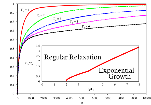
Figure 4: $\frac{Im\left(\chi_{M}^{(1)}\right)}{Im\left(\chi_{\infty}^{(1)}\right)}$. In every case $\delta=0$, $\Gamma_{R}=0$, $\Omega_{c}=1$ and $\Omega_{p}=0.1$. The absorption curves display non-linear signatures. Saturation takes place according to the interplay between decay and coupling. Inset: Relaxation map for $M>1$. The case $M=1$ shows no signatures of exponential growth.

can be integrated into a programming routine that recursively calculates the state coefficients and then $\chi_{M}^{(n)}$. We note that when $|\Gamma_{e}-\Gamma_{R}|<<2\Omega_{c}k$ the recursion matrix can be approximated as follows,

$$\hat{A}_{k}\approx\left(\begin{array}[]{cc}\frac{-1}{i\Gamma_{e}+\delta}&0\\ 0&\frac{-1}{i\Gamma_{e}+\delta}\end{array}\right).$$ (46)

Employing this $\hat{A}_{k}$ one finds a stationary state displaying the following susceptibility [29],

$$\chi_{\infty}^{(1)}=\frac{-\Omega_{p}}{(i\Gamma_{e}+\delta)},\hskip 14.22636pt\chi_{\infty}^{(2)}=\left(\chi_{\infty}^{(1)}\right)^{2}.$$ (47)

Similarly, from a direct calculation the single particle susceptibility is found to be,

$$\chi_{1}^{(1)}=\frac{-\Omega_{p}(i\Gamma_{R}+\delta)}{(i\Gamma_{R}+\delta)(i\Gamma_{e}+\delta)-\Omega_{c}^{2}}.$$ (48)

As can be seen in figure 3, equations (47) and (48) are extreme cases of the numerical results obtained using the matrix $\hat{A}_{k}$ recursively. Here we have chosen the case $\Gamma_{R}=0$ because it is most close to the actual experimental case where the decay rate of the Rydberg state is usually negligible. The inclusion of more particles in the system induces a rise of $Im\left(\chi_{M}^{(1)}\right)$ at zero detuning. In the same instance, $Re\left(\chi_{M}^{(2)}\right)$ undergoes a change of sign as it dips from its peaking value. From figure 4 we can see that the absorption profile at $\delta=0$ features non-linear behaviour over a wide range of values of $M$ and then asymptotically converges toward the estimation given by equation (47). As we increase $\Gamma_{e}$, the growth speed decreases and the curves display stronger inflection. In every case the absorption profile is characterised by a steep absorption growth. Such a non-linear response is linked to a cooperative many-body state where the single particle outcome is no longer dominant. As $M$ goes up further, the absorption value starts to saturate, suggesting that less particles are being integrated in the interaction process.

In the single particle case, maximal transmission is achieved as a result of almost perfect quantum interference between excitation pathways. In this case the only coupling mode involved in EIT in equations (8-12) is $n=0$. Gradual increase of $\Omega_{p}$ allows more particles into the excited band and therefore more coupling modes participate in the EIT process. One important characteristic of EIT is that the reduction of absorption at zero detuning is accompanied by a peak in the refraction coefficient[1]. This allows for powerful applications such as slow light or light storage. The mechanism behind the latter procedures is based on the fact that at $\delta=0$ absorption can be made low at the same time that the coefficient that determines the velocity of light in the medium peaks. This important property can be observed without much effort using our approach. Figure 3a shows a dip in $Im\left(\chi_{M}^{(1)}\right)$ while figure 3b shows and a peak in $Re\left(\chi_{M}^{(2)}\right)$ for the same parameters. Also at single-photon resonance it can be shown that independently of $M$,

$$Re\left(\chi_{M}^{(1)}\right)_{\delta=0}=Im\left(\chi_{M}^{(2)}\right)_{\delta=0}=0,$$ (49)

Notice that the peaking of refraction can only be seen for $M>1$ because $\chi_{1}^{(2)}=0$. This means that the system’s refraction at $\delta=0$ depends only on two-or-more-body transitions, where several atoms are excited (or decay) simultaneously. In a sense, one can think of the process taking place at zero detuning as one in which single-body transitions play a rather marginal role and instead the leading response is mediated by higher order transitions. Likewise, coupling modes involving more than one particle display less interference, as many particle pathways between the ground- and excited-bands can only interfere partially with their blockade counterparts.

As even more atoms are integrated in the model, the possibilities of light being absorbed via particle excitation become higher and the characteristic profile of EIT finally fades away. The enhancement of absorption due to many-body effects is especially notorious in the range $M<1000$. Since the peak of refraction at $M=2$ is positive one can find a value of $M$ ($M=65$ for the values of figure 3) for which refraction is almost zero at zero-detuning, while absorption is still low. In this case the system is almost unresponsive to the incoming radiation.

In order to check for the consistency of our approach we stress that our central assumption is the cancellation of $\hat{\kappa}(t)$ in equation (19) as $t\rightarrow\infty$. This is indeed the case as long as all the imaginary parts of the arguments of the exponentials in equation (19) turn out to be negative. Only the following arguments could become greater than zero,

$$Im(E_{n+1}^{+}-E_{n}^{-})=\frac{1}{2}\left(D(n)+D(n+1)\right)-\Gamma_{e},$$ (50)

and,

$$Im(E_{n+1}^{-}-E_{n}^{-})=\frac{1}{2}\left(D(n)-D(n+1)\right)-\Gamma_{e},$$ (51)

where,

$$D(n)=Re\left(\sqrt{(\Gamma_{e}-\Gamma_{R})^{2}-4\Omega_{c}^{2}(n+1)}\right),$$ (52)

for $n=2,3,\cdots,\infty$.

If either (50) or (51) become positive then operator $\hat{\kappa}(t)$ will display exponential growth and will dominate the stationary state. While it seems operationally possible to obtain such a state, this feature is less consistent with our initial consideration in which $\Omega_{p}$ is a perturbative parameter and hence most particles remain in the ground band. Due to the form of $D(n)$, the maximum value of (50) and (51) takes place at $n=2$. Therefore, if either (50) or (51) are positive for any $n>2$ then they are positive for $n=2$ as well. Hence $n=2$ is the only relevant mode in a relaxation analysis. We have depicted in the inset of figure 4 the relaxation map that results following the arguments discussed above. It is worth pointing out that any arbitrary set of realistic parameters in which $\Gamma_{e}>\Gamma_{R}$ fall well inside the regular relaxation zone. It also becomes apparent that in the many-body case the mere existence of a dark state does not guarantee the state convergence toward such a state.

We have investigated the reduction of transparency in an EIT set-up as a result of the collective character developed by many-body matter. Results corresponding to a semi-classical model were obtained from numerical diagonalisation as well as from a perturbative approach. In the latter case we presented a semi-analytical procedure that can be used to find the stationary state of the system in the limit of small intensity of the probe laser. We have also studied the range of validity of our method and established explicit conditions for regular relaxation. The procedure itself shows interesting issues and is valid in the range of realistic experimental parameters. We have in this way presented an alternative analysis of the effects of many-body interaction on EIT. As a prospect extension of the present work, it would be interesting to introduce a light mode to describe the probe laser in order to explore the evolution of initially-coherent states of light and the effect of particle interaction on photons.

The author thanks C. Adams and J. Otterbach for their comments and C. Hadley for language advice. Financial support from the project grants (R-144-000-276-112) and (R-710-000-016-271) is acknowledged.

References

- [1] M. Fleishchhauer, A. Imamoglu and J.P. Marangos, Rev. Mod. Phys. 77, 633 (2005).
- [2] F. Renzoni, A. Lindner and E. Arimondo, Phys. Rev. A, 60, 450 (1999).
- [3] P. Plötz, J. Madroñero and S. Wimberger, J. Phys. B: At. Mol. Opt. Phys. 43, 081001 (2010).
- [4] A.V. Gorshkov, J. Otterbach, M. Fleischhauer, T. Pohl and M. D. Lukin, arXiv:1103:3700.
- [5] J.D. Pritchard, A. Gauguet, K.J. Weatherill, M.P.A. Jones and C.S. Adams, Phys. Rev. Lett. 105, 193603 (2010).
- [6] H. Schempp, G. Gunter, C.S. Hofmann, C. Giese, S.D. Saliba, B.D. DePaola, T. Amthor, M. Weidemüller, S. Sevinçli and T. Pohl, Phys. Rev. Lett. 104, 173602 (2010).
- [7] H.Z. Wu, Z.B. Yang and S.B. Zheng, Phys. Rev. A 82, 034307 (2007).
- [8] M. Müller, I. Lesanovsky, H. Weimer, H.P. Büchler and P. Zoller, Phys. Rev. Lett. 102, 170502 (2009).
- [9] L. Isenhower, E. Urban, X.L. Zhang, A.T. Gill, T. Henage, T.A. Johnson, T.G. Walker and M. Saffman. Phys. Rev. Lett. 104, 010503 (2010).
- [10] E. Shahmoon, G. Kurizki, M. Fleischhauer and D. Petrosyan, Phys. Rev. A 83, 033806 (2011).
- [11] I. Friedler, D. Petrosyan, M. Fleischhauer, G. Kurizki, Phys. Rev. A 72, 043803 (2005).
- [12] C. Guerlin, E. Brion, T. Esslinger and K. Mølmer, Phys. Rev. A, 82, 053832 (2010).
- [13] H. Yuan, L.F. Wei, J.S. Huang, X.H. Wang and V. Vedral, arXiv:1101.2550.
- [14] T. Wilk, A. Gaëtan, C. Evellin, J. Wolters, Y. Miroshnychenko, P. Grangier and A. Browaeys, Phys. Rev. Lett. 104, 010502 (2010).
- [15] J. Gillet, G.S. Agarwal and T. Bastin, Phys. Rev. A 81, 013837 (2010).
- [16] Y. Li, L. Aolita and L.C. Kwek, Phys. Rev. A 83, 032313 (2011).
- [17] D. Møller, L.B. Madsen and K. Mølmer, Phys. Rev. Lett. 100, 170504 (2008).
- [18] I.I. Beterov, D.B. Tretyakov, V.M. Entin, E.A. Yakshina, I.I. Ryabtsev, C. MacCormick and S. Bergamini, arXiv:1102.5223.
- [19] M. Saffman, T.G. Walker and K. Mølmer, Rev. Mod. Phys. 82, 2313 (2010).
- [20] D. Petrosyan, J. Otterbach, and M. Fleischhauer, arXiv:1106.1360.
- [21] S. Sevinçli, N. Henkel, C. Ates, and T. Pohl, arXiv:1106.2001.
- [22] C. Ates, S. Sevinçli and T. Pohl, Phys. Rev. A 83, 041802 (2011).
- [23] J. Gong and S. Rice, Phys. Rev. A, 69, 063410 (2004).
- [24] J. Gong and S. Rice, J. Chem. Phys., 120, 5117 (2004).
- [25] E.M. Graefe, H.J. Korsch and A.E. Niederle, Phys. Rev. Lett., 101, 150408 (2008).
- [26] V.S. Shchesnovich and D.S. Mogilevtsev, Phys. Rev. A, 82, 043621 (2010).
- [27] S.L. Cornish, N.R. Claussen, J.L. Roberts, E.A. Cornell and C.E. Wieman, Phys. Rev. Lett. 85, 1795 (2000).
- [28] Here we abuse the standard notation and use the bra symbol to make reference to the left eigenvector of the NHH.
- [29] In order to facilitate the presentation of equations (47) and (48) we omit a normalisation factor of order . This is not the case when the same formulae are used in figure 3.