LPHE-MS-11-01 / CPM-11-01


Four Dimensional Graphene

L.B Drissi 1,2, E.H Saidi 2,3,4, M. Bousmina 2

1International Centre for Theoretical Physics, ICTP, Trieste, Italy,
2MAScIR, Institute of Nanomaterials and Nanotechnology, ENSET, Rabat, Morocco
3LPHE-Modeling and Simulation, Faculté des Sciences, Rabat, Morocco
4Centre of Physics and Mathematics, CPM- CNESTEN, Morocco
Abstract

Mimicking pristine 2D graphene, we revisit the BBTW model  for 4D lattice QCD given in [P. F. Bedaque et al. Phys. Rev. D78 (2008) 017502] by using the hidden $SU\left(5\right)$ symmetry of the 4D hyperdiamond lattice $\mathcal{H}_{4}$. We first study the link between the $\mathcal{H}_{4}$ and $SU\left(5\right)$; then we refine the BBTW 4D lattice action by using the weight vectors $\mathbf{\lambda}_{1},$ $\mathbf{\lambda}_{2},$ $\mathbf{\lambda}_{3},$ $\mathbf{\lambda}_{4},$ $\mathbf{\lambda}_{5}$ of the 5-dimensional representation of $SU\left(5\right)$ satisfying $\sum_{i}\mathbf{\lambda}_{i}=0$. After that we study explicitly the solutions of the zeros of the Dirac operator $\mathcal{D}$ in terms of the SU$\left(5\right)$ simple roots $\mathbf{\alpha}_{1},$ $\mathbf{\alpha}_{2},$ $\mathbf{\alpha}_{3},$ $\mathbf{\alpha}_{4}$ generating $\mathcal{H}_{4}$; and its fundamental weights $\omega_{1},$ $\omega_{2},$ $\omega_{3},$ $\omega_{4}$ which generate the reciprocal lattice $\mathcal{H}_{4}^{\ast}$. It is shown, amongst others, that these zeros live at the sites of $\mathcal{H}_{4}^{\ast}$; and the continuous limit $\mathcal{D}$ is given by $\frac{id\sqrt{5}}{2}$ $\gamma^{\mu}\mathbf{k}_{\mu}$ with $d,$ $\gamma^{\mu}$ and $\mathbf{k}_{\mu}$ standing respectively for the lattice parameter of $\mathcal{H}_{4}$, the usual 4 Dirac matrices and the 4D wave vector. Other features such as differences with BBTW model as well as the link between the Dirac operator following from our construction and the one suggested by Creutz using quaternions, are also given.


Keywords: Graphene, Lattice QCD, 4D hyperdiamond, BBTW model, $SU\left(5\right)$ Symmetry.

1 Introduction

In the last few years, there have been attempts to extend results on the relativistic electron system on a 2D honeycomb (graphene) [1, 2, 3] to a 4D honeycomb lattice (called 4D hyperdiamond, denoted below as $\mathcal{H}_{4}$) and apply it to the lattice QCD simulations [4]-[13]. These attempts try to construct Dirac fermion on $\mathcal{H}_{4}$ by keeping all desirable properties; in particular locality, chiral symmetry and the minimal number of fermion doublings [4, 8]; see also [12] and refs therein. In this regards, two remarkable approaches were given, first by Creutz suggesting an extension of graphene dispersion relations by using quaternions [4, 8]; and subsequently by Bedaque-Bachoff-Tiburzi-WalkerLoud (BBTW) [5] proposing a 4D hyperdiamond lattice action with enough symmetries to exclude fine tuning. Apparently those two attempts look very close since both of them extend 2D graphene to 4D; however they have basic differences; some of them are discussed in [5]. The Creutz model involves a two parameter lattice action that lives on a distorted 4D lattice; and so looses the high discrete symmetry of the 4D hyperdiamond. The lattice action of BBTW model extends pristine 2D graphene; it is built on perfect 4D hyperdiamond and has sufficient discrete symmetries for a good continuum limit. Nevertheless, in both Creutz and BBTW constructions, the distorted and perfect 4D hyperdiamonds are thought of as made by the superposition of two sublattices $\mathcal{A}_{4}$ and $\mathcal{B}_{4}$ with massless left and right-handed fermions as required by the no-go theorems for lattice chiral symmetry [14, 15].
Guided by the rich symmetries of the 4D hyperdiamond $\mathcal{H}_{4}$, we revisit in this paper, the BBTW model of ref [5] and its higher dimension extensions given in [12] by using the hidden $SU\left(5\right)$ [ resp. $SU\left(d+1\right)$] symmetry of $\mathcal{H}_{4}$ [ resp. $\mathcal{H}_{d+1}$ ] and its reciprocal lattice $\mathcal{H}_{4}^{\ast}$ [ resp. $\mathcal{H}_{d+1}^{\ast}$ ]. Focussing on 4D lattice QCD, we first review the link between BBTW construction and $SU\left(5\right)$. Then we refine the hyperdiamond lattice action by using the weight vectors $\mathbf{\lambda}_{1},$ $\mathbf{\lambda}_{2},$ $\mathbf{\lambda}_{3},$ $\mathbf{\lambda}_{4},$ $\mathbf{\lambda}_{5}$ of the 5-dimensional (fundamental) representation of $SU\left(5\right)$ as well as mimicking pristine 2D graphene which, in the language of groups, corresponds precisely to $SU\left(3\right)$. After that, we study explicitly the solutions of the zeros of the Dirac operator by using the $SU\left(5\right)$ simple roots $\mathbf{\alpha}_{1},$ $\mathbf{\alpha}_{2},$ $\mathbf{\alpha}_{3},$ $\mathbf{\alpha}_{4}$ generating $\mathcal{H}_{4}$; and its fundamental weights $\omega_{1},$ $\omega_{2},$ $\omega_{3},$ $\omega_{4}$ generating the reciprocal lattice $\mathcal{H}_{4}^{\ast}$. We also comment the differences with BBTW construction; and exhibit the link between the Dirac operator, following from our approach, and the one suggested by Creutz using quaternions.
The presentation is as follows: In section 2, we review briefly the BBTW parametrization of the real 4D hyperdiamond $\mathcal{H}_{4}$ and comment some particular discrete symmetries. In section 3, we study the link  between $\mathcal{H}_{4}$ and the SU$\left(5\right)$ symmetry. It is shown that $\mathcal{H}_{4}$ is precisely generated by the four simple roots $\mathbf{\alpha}_{1},$ $\mathbf{\alpha}_{2},$ $\mathbf{\alpha}_{3},$ $\mathbf{\alpha}_{4}$ of $SU\left(5\right)$; and the reciprocal lattice $\mathcal{H}_{4}^{\ast}$ is generated by its four weight vectors $\mathbf{\omega}_{1},$ $\mathbf{\omega}_{2},$ $\mathbf{\omega}_{3},$ $\mathbf{\omega}_{4}$. In section 4, we revisit the BBTW model on $\mathcal{H}_{4}$ given in [5] and propose a refined 4D lattice action mimicking perfectly 2D graphene. In section 5, we study explicitly the zeros of the Dirac operator; and in section 6 we re-derive the Boriçi-Creutz fermions. In last section, we give a conclusion and make comments regarding other lattice models.

2 4D hyperdiamond $\mathcal{H}_{4}$

Seen that the 4D hyperdiamond $\mathcal{H}_{4}$ plays a central role in both BBTW and Creutz lattice models [4, 5], we start by studying this 4D lattice by exhibiting explicitly its crystallographic structure. In particular, we give the relative positions of the 5 first and the 20 second nearest neighbors and exhibit some particular discrete symmetries of $\mathcal{H}_{4}$.
This analysis, which is useful in studying the link between the lattices $\mathcal{H}_{4}$ and the $SU\left(5\right)$ simple roots, is important in our construction; it will be used in section 3 to build the reciprocal lattice $\mathcal{H}_{4}^{\ast}$ and in section 5 to study the dispersion energy relations as well as the zeros of the Dirac operator.

2.1 BBTW parametrization of $\mathcal{H}_{4}$

In order to apply graphene simulation methods to lattice QCD, BBTW generalizes tight binding model of 2D graphene to the 4D diamond $\mathcal{H}_{4}$ [5, 6]; see also [7, 8, 9, 10]. Like in the case of 2D honeycomb, this 4D lattice is defined by two superposed sublattices $\mathcal{A}_{4}$ and $\mathcal{B}_{4}$ with the two following basic objects:
First, sites in $\mathcal{A}_{4}$ and $\mathcal{B}_{4}$ (L-nodes and R-nodes in the terminology of [5]) are parameterized by the typical 4d- vectors $\mathbf{r}_{\mathbf{n}}$ with $\mathbf{n}=\left({\small n}_{1}{\small,n}_{2}{\small,n}_{3}{\small,n}_{4}\right)$ and ${\small n}_{i}$’s arbitrary integers. These lattice vectors are expanded as follows

$\mathcal{A}_{4}$ : $\mathbf{r}_{\mathbf{n}}=n_{1}$ $\mathbf{a}_{1}+n_{2}$ $\mathbf{a}_{2}+n_{3}$ $\mathbf{a}_{3}+n_{4}$ $\mathbf{a}_{4}$ ,
$\mathcal{B}_{4}$ : $\mathbf{r}_{\mathbf{n}}^{\prime}=\mathbf{r}_{\mathbf{n}}+\mathbf{e}$ ,
(2.1)

where $\mathbf{a}_{1},$ $\mathbf{a}_{2},$ $\mathbf{a}_{3},$ $\mathbf{a}_{4}$ are primitive vectors generating these sublattices; and $\mathbf{e}$ is a shift vector as described in what follows.
Second, the vector $\mathbf{e}$ is a global vector taking the same value $\forall$ $\mathbf{n}$; it is a shift vector giving the relative positions of the $\mathcal{B}_{4}$ sites with respect to the $\mathcal{A}_{4}$ ones; i.e: $\mathbf{e=r}_{\mathbf{n}}^{\prime}-\mathbf{r}_{\mathbf{n}}$, $\forall$ $\mathbf{n}$. In ref.[5], the $\mathbf{a}_{l}$’s and the $\mathbf{e}$ have been chosen as given by the following 4- component vectors

$\mathbf{a}_{1}$ $=\mathbf{e}_{1}-\mathbf{e}_{5}$ , $\mathbf{a}_{3}$ $=\mathbf{e}_{3}-\mathbf{e}_{5}$ , $\mathbf{e}$ $=\mathbf{e}_{5}$ ,
$\mathbf{a}_{2}$ $=\mathbf{e}_{2}-\mathbf{e}_{5}$ , $\mathbf{a}_{4}$ $=\mathbf{e}_{4}-\mathbf{e}_{5}$
(2.2)

with the representation

$\mathbf{e}_{1}^{\mu}$ $=\frac{1}{4}\left(+\sqrt{5},+\sqrt{5},+\sqrt{5},+1\right)$ ,
$\mathbf{e}_{2}^{\mu}$ $=\frac{1}{4}\left(+\sqrt{5},-\sqrt{5},-\sqrt{5},+1\right)$ ,
$\mathbf{e}_{3}^{\mu}$ $=\frac{1}{4}\left(-\sqrt{5},-\sqrt{5},+\sqrt{5},+1\right)$ ,
$\mathbf{e}_{4}^{\mu}$ $=\frac{1}{4}\left(-\sqrt{5},+\sqrt{5},-\sqrt{5},+1\right)$ ,
(2.3)

and

$\mathbf{e}_{5}^{\mu}$ $=-\mathbf{e}_{1}^{\mu}-\mathbf{e}_{2}^{\mu}-\mathbf{e}_{3}^{\mu}-\mathbf{e}_{4}^{\mu}$ $=\left(\text{ \ }0,\text{ \ }0,\text{ \ }0,\text{ \ }-1\right)$.
(2.4)

Notice also that the 5 vectors $\mathbf{e}_{1},$ $\mathbf{e}_{2},$ $\mathbf{e}_{3},$ $\mathbf{e}_{4},$ $\mathbf{e}_{5}$ define the first nearest neighbors to $\left(0,0,0,0\right)$ and satisfy the constraint relations,

$\mathbf{e}_{i}.\mathbf{e}_{i}$ $=\sum e_{i}^{\mu}.e_{i}^{\mu}=\sum e_{i\mu}.e_{i}^{\mu}=1$
$\mathbf{e}_{i}.\mathbf{e}_{j}$ $=\cos\vartheta_{ij}=-\frac{1}{4},\quad i\neq j$ ,
(2.5)

showing that the $\mathbf{e}_{i}$’s are distributed in a symmetric way since all the angles $\vartheta_{ij}$ are equal to $\arccos\left(-\frac{1}{4}\right)$; see also figure (1) for illustration.
In the matrix representation (2.3-2.4), the free four vectors $\mathbf{e}_{1},$ $\mathbf{e}_{2},$ $\mathbf{e}_{3},$ $\mathbf{e}_{4}$ are permuted amongst each others by the typical unimodular matrices $\mathcal{O}_{{}_{\left[ij\right]}}$ acting as

$\mathbf{e}_{i}^{\mu}=\mathop{\displaystyle\sum}\limits_{\nu=1}^{4}\left(\mathcal{O}_{{}_{\left[ji\right]}}\right)_{\nu}^{\mu}\mathbf{e}_{j}^{\nu},$ $i,j=1,2,3,4,$
(2.6)

with,

$\mathcal{O}_{{}_{\left[21\right]}}=\left(\begin{array}[]{cccc}1&0&0&0\\ 0&-1&0&0\\ 0&0&-1&0\\ 0&0&0&1\end{array}\right)$, $\mathcal{O}_{{}_{\left[32\right]}}=\left(\begin{array}[]{cccc}-1&0&0&0\\ 0&1&0&0\\ 0&0&-1&0\\ 0&0&0&1\end{array}\right).$
(2.7)

These transformations leave invariant the vector $\mathbf{e}_{5}=-\left(\mathbf{e}_{1}+\mathbf{e}_{2}+\mathbf{e}_{3}+\mathbf{e}_{4}\right)$; they are sub-symmetries of the permutation group generated by permutations of the five $\mathbf{e}_{i}$’s. We also have

$\mathcal{O}_{{}_{\left[21\right]}}$ $=\mathcal{O}_{{}_{\left[43\right]}}$ , $\mathcal{O}_{{}_{\left[31\right]}}$ $=\mathcal{O}_{{}_{\left[32\right]}}\mathcal{O}_{{}_{\left[21\right]}}$
$\mathcal{O}_{{}_{\left[32\right]}}$ $=\mathcal{O}_{{}_{\left[14\right]}}$ , $\mathcal{O}_{{}_{\left[41\right]}}$ $=\mathcal{O}_{{}_{\left[43\right]}}\mathcal{O}_{{}_{\left[31\right]}}$
(2.8)

together with other similar relations.

2.2 Some specific properties

From the figure (1) representing the first nearest neighbors in the 4D hyperdiamond and their analog in 2D graphene, we learn that each $\mathcal{A}_{4}$- type node at $\mathbf{r}_{\mathbf{n}}$, with some attached wave function $A_{\mathbf{r}_{\mathbf{n}}}$, has the following closed neighbors:

Refer to caption
Figure 1: On left the 5 first nearest neighbors in the pristine 4D hyperdiamond with the properties $\left\|\mathbf{e}_{i}\right\|=1$ and $\mathbf{e}_{1}+\mathbf{e}_{2}+\mathbf{e}_{3}+\mathbf{e}_{4}+\mathbf{e}_{5}=0$. On right, the 3 first nearest in pristine 2D graphene with $\left\|\mathbf{e}_{i}\right\|=1$ and $\mathbf{e}_{1}+\mathbf{e}_{2}+\mathbf{e}_{3}=0$.

5 first nearest neighbors belonging to $\mathcal{B}_{4}$ with wave functions $B_{\mathbf{r}_{\mathbf{n}}+d\mathbf{e}_{i}}$; and 20 second nearest neighbors belonging to the same $\mathcal{A}_{4}$ with the wave functions $A_{\mathbf{r}_{\mathbf{n}}+d\left(\mathbf{e}_{i}-\mathbf{e}_{j}\right)}$. The first nearest neighbors are given by:

lattice position attached wave
$\ \ \ \mathbf{r}_{\mathbf{n}}+d\mathbf{e}_{1}$ $\longleftrightarrow$ $\ \ \ B_{\mathbf{r}_{\mathbf{n}}+d\mathbf{e}_{1}}$
$\ \ \ \mathbf{r}_{\mathbf{n}}+d\mathbf{e}_{2}$ $\longleftrightarrow$ $\ \ \ B_{\mathbf{r}_{\mathbf{n}}+d\mathbf{e}_{2}}$
$\ \ \ \mathbf{r}_{\mathbf{n}}+d\mathbf{e}_{3}$ $\longleftrightarrow$ $\ \ \ B_{\mathbf{r}_{\mathbf{n}}+d\mathbf{e}_{3}}$
$\ \ \ \mathbf{r}_{\mathbf{n}}+d\mathbf{e}_{4}$ $\longleftrightarrow$ $\ \ \ B_{\mathbf{r}_{\mathbf{n}}+d\mathbf{e}_{4}}$
$\ \ \ \mathbf{r}_{\mathbf{n}}+d\mathbf{e}_{5}$ $\longleftrightarrow$ $\ \ \ B_{\mathbf{r}_{\mathbf{n}}+d\mathbf{e}_{5}}$
(2.9)

Using this configuration, the typical tight binding hamiltonian describing the couplings between the first nearest neighbors reads as

$-t\mathop{\displaystyle\sum}\limits_{\mathbf{r}_{\mathbf{n}}}\mathop{\displaystyle\sum}\limits_{i=1}^{5}A_{\mathbf{r}_{\mathbf{n}}}B_{\mathbf{r}_{\mathbf{n}}+d\mathbf{e}_{i}}^{+}+hc$ .
(2.10)

where $t$ is the hop energy and where $d$ is the lattice parameter. Notice that in the case where the wave functions at $\mathbf{r}_{\mathbf{n}}$ and $\mathbf{r}_{\mathbf{n}}+d\mathbf{e}_{i}$ are rather given by two component Weyl spinors

$A_{\mathbf{r}_{\mathbf{n}}}^{a}=\left(\begin{array}[]{c}A_{\mathbf{r}_{\mathbf{n}}}^{1}\\ A_{\mathbf{r}_{\mathbf{n}}}^{2}\end{array}\right)$ , $\bar{B}_{\mathbf{r}_{\mathbf{n}}+d\mathbf{e}_{i}}^{\dot{a}}=\left(\begin{array}[]{c}\bar{B}_{\mathbf{r}_{\mathbf{n}}+d\mathbf{e}_{i}}^{\dot{1}}\\ \bar{B}_{\mathbf{r}_{\mathbf{n}}+d\mathbf{e}_{i}}^{\dot{2}}\end{array}\right)$ ,
(2.11)

together with their adjoints $\bar{A}_{\mathbf{r}_{\mathbf{n}}}^{\dot{a}}$ and $\bar{B}_{\mathbf{r}_{\mathbf{n}}+d\mathbf{e}_{i}}^{a}$, as in the example of 4D lattice QCD to be described in section 4, the corresponding tight binding model would be,

$-t\mathop{\displaystyle\sum}\limits_{\mathbf{r}_{\mathbf{n}}}\mathop{\displaystyle\sum}\limits_{i=1}^{5}\left[\mathop{\displaystyle\sum}\limits_{\mu=1}^{4}\mathbf{e}_{i}^{\mu}\left(A_{\mathbf{r}_{\mathbf{n}}}^{a}\mathrm{\sigma}_{a\dot{a}}^{\mu}\bar{B}_{\mathbf{r}_{\mathbf{n}}+d\mathbf{e}_{i}}^{\dot{a}}\right)\right]+hc$ .
(2.12)

where the $\mathbf{e}_{i}^{\mu}$’s are as in (2.3) and where the coefficients $\mathrm{\sigma}_{a\dot{a}}^{\mu}$ will be specified later on. Notice moreover that the term $\sum_{i=1}^{5}\mathbf{e}_{i}^{\mu}\left(A_{\mathbf{r}_{\mathbf{n}}}^{a}\mathrm{\sigma}_{a\dot{a}}^{\mu}\bar{B}_{\mathbf{r}_{\mathbf{n}}}^{\dot{a}}\right)$ vanishes identically due to $\sum_{i=1}^{5}\mathbf{e}_{i}^{\mu}=0.$ The 20 second nearest neighbors read as

${\small r}_{\mathbf{n}}\pm d\left(\mathbf{e}_{1}-\mathbf{e}_{2}\right){\small,}$ ${\small r}_{\mathbf{n}}\pm d\left(\mathbf{e}_{1}-\mathbf{e}_{3}\right){\small,}$ ${\small r}_{\mathbf{n}}\pm d\left(\mathbf{e}_{1}-\mathbf{e}_{4}\right){\small,}$
${\small r}_{\mathbf{n}}\pm d\left(\mathbf{e}_{1}-\mathbf{e}_{5}\right){\small,}$ ${\small r}_{\mathbf{n}}\pm d\left(\mathbf{e}_{2}-\mathbf{e}_{3}\right){\small,}$ ${\small r}_{\mathbf{n}}\pm d\left(\mathbf{e}_{2}-\mathbf{e}_{4}\right){\small,}$
${\small r}_{\mathbf{n}}\pm d\left(\mathbf{e}_{2}-\mathbf{e}_{5}\right){\small,}$ ${\small r}_{\mathbf{n}}\pm d\left(\mathbf{e}_{3}-\mathbf{e}_{4}\right){\small,}$ ${\small r}_{\mathbf{n}}\pm d\left(\mathbf{e}_{3}-\mathbf{e}_{5}\right){\small,}$
${\small r}_{\mathbf{n}}\pm d\left(\mathbf{e}_{4}-\mathbf{e}_{5}\right){\small.}$
(2.13)

At this order, the standard tight binding hamiltonian reads as follows

$-t^{\prime}\mathop{\displaystyle\sum}\limits_{\mathbf{r}_{\mathbf{n}}}\mathop{\displaystyle\sum}\limits_{i,j=1}^{5}\left(A_{\mathbf{r}_{\mathbf{n}}}A_{\mathbf{r}_{\mathbf{n}}+d\left(\mathbf{e}_{i}-\mathbf{e}_{j}\right)}^{+}+B_{\mathbf{r}_{\mathbf{n}}}B_{\mathbf{r}_{\mathbf{n}}+d\left(\mathbf{e}_{i}-\mathbf{e}_{j}\right)}^{+}\right)+hc$ .
(2.14)

and in the case of Weyl spinors, we have

$$-t^{\prime}\mathop{\displaystyle\sum}\limits_{\mathbf{r}_{\mathbf{n}}}\mathop{\displaystyle\sum}\limits_{i,j=1}^{5}\left[\mathop{\displaystyle\sum}\limits_{\mu=1}^{4}\mathbf{e}_{i}^{\mu}\left(A_{\mathbf{r}_{\mathbf{n}}}^{a}\mathrm{\sigma}_{a\dot{a}}^{\mu}\bar{A}_{\mathbf{r}_{\mathbf{n}}+d\left(\mathbf{e}_{i}-\mathbf{e}_{j}\right)}^{\dot{a}}+B_{\mathbf{r}_{\mathbf{n}}}^{a}\mathrm{\sigma}_{a\dot{a}}^{\mu}\bar{B}_{\mathbf{r}_{\mathbf{n}}+d\left(\mathbf{e}_{i}-\mathbf{e}_{j}\right)}^{\dot{a}}\right)\right]+hc$$ (2.15)

In what follows, we show that the 5 vectors $\mathbf{e}_{1},$ $\mathbf{e}_{2},$ $\mathbf{e}_{3},$ $\mathbf{e}_{4}$ $\mathbf{e}_{5}$ are, up to a normalization factor namely $\frac{\sqrt{5}}{2}$, precisely the weight vectors $\mathbf{\lambda}_{0},$ $\mathbf{\lambda}_{1},$ $\mathbf{\lambda}_{2},$ $\mathbf{\lambda}_{3},$ $\mathbf{\lambda}_{4}$ of the 5-dimensional representation of $SU\left(5\right)$; and the 20 vectors $\left(\mathbf{e}_{i}-\mathbf{e}_{j}\right)$ are, up to a scale factor $\frac{\sqrt{5}}{2}$, their roots $\beta_{ij}=\left(\mathbf{\lambda}_{i}-\mathbf{\lambda}_{j}\right)$. We show as well that the particular property $\mathbf{e}_{i}.\mathbf{e}_{j}=-\frac{1}{4}$, which is constant $\forall$ $\mathbf{e}_{i}$, $\forall$ $\mathbf{e}_{j}$, has a natural interpretation in terms of the Cartan matrix of $SU\left(5\right)$.

3 Link with $SU\left(5\right)$ symmetry

For later use, we exhibit here the hidden $SU\left(5\right)$ symmetry of the 4D hyperdiamond; we show that $\mathcal{H}_{4}$ considered above is precisely the lattice $\mathcal{L}_{su\left(5\right)}$ studied in [16]. More concretely, we show the three following:
First, the 5 bond vectors $\mathbf{e}_{1},$ $\mathbf{e}_{2},$ $\mathbf{e}_{3},$ $\mathbf{e}_{4},$ $\mathbf{e}_{5}$ ( first nearest neighbors) are given by the 5 weight vectors $\mathbf{\lambda}_{1},$ $\mathbf{\lambda}_{2},$ $\mathbf{\lambda}_{3},$ $\mathbf{\lambda}_{4},$ $\mathbf{\lambda}_{5}$ ( below, we set $\mathbf{\lambda}_{5}\equiv\mathbf{\lambda}_{0}$) of the 5-dimensional (fundamental) representation of $SU\left(5\right)$ which also satisfy

$$\mathbf{\lambda}_{0}+\mathbf{\lambda}_{1}+\mathbf{\lambda}_{2}+\mathbf{\lambda}_{3}+\mathbf{\lambda}_{4}=0$$ (3.1)

We will show later that $\mathbf{e}_{i}=\frac{\sqrt{5}}{2}\mathbf{\lambda}_{i}$ with $\mathbf{\lambda}_{i}.\mathbf{\lambda}_{i}=\frac{4}{5}.$
Second, the 4 primitive ones $\mathbf{a}_{1},$ $\mathbf{a}_{2},$ $\mathbf{a}_{3},$ $\mathbf{a}_{4}$ used in generating $\mathcal{H}_{4}$ are particular linear combinations of the 4 simple roots $\mathbf{\alpha}_{1},$ $\mathbf{\alpha}_{2},$ $\mathbf{\alpha}_{3},$ $\mathbf{\alpha}_{4}$ of $SU\left(5\right)$; see eq(3.20) for the explicit relations. Recall that the $SU\left(5\right)$ symmetry has 20 roots as given below,

$\pm\mathbf{\alpha}_{1},$ $\pm\left(\mathbf{\alpha}_{1}+\mathbf{\alpha}_{2}\right),$ $\pm\left(\mathbf{\alpha}_{1}+\mathbf{\alpha}_{2}+\mathbf{\alpha}_{3}\right),$ $\pm\left(\mathbf{\alpha}_{1}+\mathbf{\alpha}_{2}+\mathbf{\alpha}_{3}+\mathbf{\alpha}_{4}\right)$
$\pm\mathbf{\alpha}_{2},$ $\pm\left(\mathbf{\alpha}_{2}+\mathbf{\alpha}_{3}\right),$ $\pm\left(\mathbf{\alpha}_{2}+\mathbf{\alpha}_{3}+\mathbf{\alpha}_{4}\right),$
$\pm\mathbf{\alpha}_{3},$ $\pm\left(\mathbf{\alpha}_{3}+\mathbf{\alpha}_{4}\right),$
$\pm\mathbf{\alpha}_{3}$
(3.2)

These vectors have all of them the same length $\mathbf{\alpha}^{2}=2$; and so they generate the relative lattice positions of the second nearest neighbors in the 4D hyperdiamond.
Third, the $SU\left(5\right)$ has also discrete symmetries given by the so called Weyl group transformations generated by the $\sigma_{\mathbf{\alpha}}$’s acting on generic roots $\mathbf{\beta}$ of SU$\left(5\right)$ as follows,

$\sigma_{\mathbf{\alpha}}\left(\mathbf{\beta}\right)$ $=$ $\mathbf{\beta}-2\frac{\mathbf{\alpha.\beta}}{\mathbf{\alpha}^{2}}\mathbf{\beta=\beta}-\left(\alpha.\beta\right)$ $\mathbf{\beta}$ .
(3.3)

These discrete transformations permute the roots (3.2) amongst themselves and are isomorphic to $\mathcal{S}_{5}$ permutation group transformations. For instance, we have $\sigma_{\mathbf{\alpha}_{1}}\left(\mathbf{\alpha}_{1}\right)=-\mathbf{\alpha}_{1}$ and $\sigma_{\mathbf{\alpha}_{1}}\left(\mathbf{\alpha}_{2}\right)=\mathbf{\alpha}_{1}+\mathbf{\alpha}_{2}$.

3.1 Exhibiting the link $\mathcal{H}_{4}/SU\left(5\right)$

To exhibit explicitly the link between pristine lattice $\mathcal{H}_{4}$ and the simple roots and the basic weight vectors of $SU\left(5\right)$, we start by recalling some of its features; in particular the following useful ingredients: $SU\left(5\right)$ is a 24 dimensional symmetry group; it has rank 4; that is 4 simple roots $\mathbf{\alpha}_{1},$ $\mathbf{\alpha}_{2},$ $\mathbf{\alpha}_{3},$ $\mathbf{\alpha}_{4}$; it has 20 roots $\pm\mathbf{\beta}_{ij}$ given by eq(3.2). The simple roots $\mathbf{\alpha}_{1},$ $\mathbf{\alpha}_{2},$ $\mathbf{\alpha}_{3},$ $\mathbf{\alpha}_{4}$ capture most of the algebraic properties of SU$\left(5\right)$; and as a consequence, those of the 4D hyperdiamond crystal; in particular they generate the 20 roots $\pm\mathbf{\beta}_{ij}$ as shown on (3.2) and they have a symmetric intersection matrix $\mathbf{K}_{ij}=\mathbf{\alpha}_{i}$.$\mathbf{\alpha}_{j}$ with inverse $\mathbf{K}_{ij}^{-1}$ given by,

$\mathbf{K}_{ij}=\left(\begin{array}[]{cccc}2&-1&0&0\\ -1&2&-1&0\\ 0&-1&2&-1\\ 0&0&-1&2\end{array}\right)$ , $\mathbf{K}_{ij}^{-1}=\frac{1}{5}\left(\begin{array}[]{cccc}4&3&2&1\\ 3&6&4&2\\ 2&4&6&3\\ 1&2&3&4\end{array}\right)$
(3.4)

that encode the algebraic data of the underlying Lie algebra of the $SU\left(5\right)$ symmetry. These simple roots define as well the 4 fundamental weights $\mathbf{\omega}_{1},$ $\mathbf{\omega}_{2},$ $\mathbf{\omega}_{3},$ $\mathbf{\omega}_{4}$ through the following duality relation

$\mathbf{\omega}_{i}.\mathbf{\alpha}_{j}$ $=$ $\delta_{ij},$ $i,j=1,...,4$.
(3.5)

These fundamental weights are important for us; first because they allow to build the reciprocal 4D hyperdiamond $\mathcal{H}_{4}^{\ast}$ and second can be use used to expand any wave vector in $\mathcal{H}_{4}^{\ast}$ as follows

$$\mathbf{k}=k_{1}\mathbf{\omega}_{1}+k_{2}\mathbf{\omega}_{2}+k_{3}\mathbf{\omega}_{3}+k_{4}\mathbf{\omega}_{4}.$$ (3.6)

From this expansion we read the relations $k_{i}=\mathbf{k}.\mathbf{\alpha}_{i}$ showing that the $k_{i}$’s are precisely the wave vector components propagating along the $\mathbf{\alpha}_{i}$-directions; thanks to eqs(3.5).

3.2 Other useful relations

Using the matrices $\mathbf{K}_{ij}$ and $\mathbf{K}_{ij}^{-1}$, one can express the simple roots $\mathbf{\alpha}_{i}$ in terms of the fundamental weight vectors $\mathbf{\omega}_{i}$; and inversely the $\mathbf{\omega}_{i}$’s as linear combinations of the simple roots as given below,

$\mathbf{\omega}_{1}=\frac{4}{5}\mathbf{\alpha}_{1}+\frac{3}{5}\mathbf{\alpha}_{2}+\frac{2}{5}\mathbf{\alpha}_{3}+\frac{1}{5}\mathbf{\alpha}_{4}$
$\mathbf{\omega}_{2}=\frac{3}{5}\mathbf{\alpha}_{1}+\frac{6}{5}\mathbf{\alpha}_{2}+\frac{4}{5}\mathbf{\alpha}_{3}+\frac{2}{5}\mathbf{\alpha}_{4}$
$\mathbf{\omega}_{3}=\frac{2}{5}\mathbf{\alpha}_{1}+\frac{4}{5}\mathbf{\alpha}_{2}+\frac{6}{5}\mathbf{\alpha}_{3}+\frac{3}{5}\mathbf{\alpha}_{4}$
$\mathbf{\omega}_{4}=\frac{1}{5}\mathbf{\alpha}_{1}+\frac{2}{5}\mathbf{\alpha}_{2}+\frac{3}{5}\mathbf{\alpha}_{3}+\frac{4}{5}\mathbf{\alpha}_{4}$
(3.7)

Using these relations, it is not difficult to check that they satisfy (3.5); for instance we have $\mathbf{\omega}_{1}.\mathbf{\alpha}_{1}$ $=$ $\frac{8}{5}-\frac{3}{5}=1$ and $\mathbf{\omega}_{1}.\mathbf{\alpha}_{2}$ $=$ $-\frac{4}{5}+\frac{6}{5}-\frac{2}{5}$ $=0$; and similarly for the others $\mathbf{\omega}_{2},$ $\mathbf{\omega}_{3},$ $\mathbf{\omega}_{4}$ and the intersections $\mathbf{\omega}_{i}.\mathbf{\alpha}_{j}$. Notice moreover that the fundamental weight vector $\mathbf{\omega}_{1}$ defines a highest weight representation of $SU\left(5\right)$ of dimension 5 with weight vectors $\mathbf{\lambda}_{0},$ $\mathbf{\lambda}_{1},$ $\mathbf{\lambda}_{2},$ $\mathbf{\lambda}_{3},$ $\mathbf{\lambda}_{4}$ related to $\mathbf{\omega}_{1}$ as follows

$\mathbf{\lambda}_{0}$ $=$ $\mathbf{\omega}_{1}$ ,
$\mathbf{\lambda}_{1}$ $=$ $\mathbf{\omega}_{1}-\mathbf{\alpha}_{1}$ ,
$\mathbf{\lambda}_{2}$ $=$ $\mathbf{\omega}_{1}-\mathbf{\alpha}_{1}-\mathbf{\alpha}_{2}$ ,
$\mathbf{\lambda}_{3}$ $=$ $\mathbf{\omega}_{1}-\mathbf{\alpha}_{1}-\mathbf{\alpha}_{2}-\mathbf{\alpha}_{3}$ ,
$\mathbf{\lambda}_{4}$ $=$ $\mathbf{\omega}_{1}-\mathbf{\alpha}_{1}-\mathbf{\alpha}_{2}-\mathbf{\alpha}_{3}-\mathbf{\alpha}_{4}$ .
(3.8)

By using (3.7), one may also express these vectors weights in terms of the $\mathbf{\omega}_{i}$’s as follows

$\mathbf{\lambda}_{0}$ $=$ $\mathbf{\omega}_{1}$ ,
$\mathbf{\lambda}_{1}$ $=$ $\mathbf{\omega}_{2}-\mathbf{\omega}_{1}$ ,
$\mathbf{\lambda}_{2}$ $=$ $\mathbf{\omega}_{3}-\mathbf{\omega}_{2}$ ,
$\mathbf{\lambda}_{3}$ $=$ $\mathbf{\omega}_{4}-\mathbf{\omega}_{3}$ ,
$\mathbf{\lambda}_{4}$ $=$ $-\mathbf{\omega}_{4}$ .
(3.9)

Furthermore, substituting $\mathbf{\omega}_{1}$ by its expression (3.7), we get the following values of the $\mathbf{\lambda}_{i}$’s in terms of the simple roots

$\mathbf{\lambda}_{0}=+\frac{4}{5}\mathbf{\alpha}_{1}+\frac{3}{5}\mathbf{\alpha}_{2}+\frac{2}{5}\mathbf{\alpha}_{3}+\frac{1}{5}\mathbf{\alpha}_{4}$ ,
$\mathbf{\lambda}_{1}=-\frac{1}{5}\mathbf{\alpha}_{1}+\frac{3}{5}\mathbf{\alpha}_{2}+\frac{2}{5}\mathbf{\alpha}_{3}+\frac{1}{5}\mathbf{\alpha}_{4}$ ,
$\mathbf{\lambda}_{2}=-\frac{1}{5}\mathbf{\alpha}_{1}-\frac{2}{5}\mathbf{\alpha}_{2}+\frac{2}{5}\mathbf{\alpha}_{3}+\frac{1}{5}\mathbf{\alpha}_{4}$ ,
$\mathbf{\lambda}_{3}=-\frac{1}{5}\mathbf{\alpha}_{1}-\frac{2}{5}\mathbf{\alpha}_{2}-\frac{3}{5}\mathbf{\alpha}_{3}+\frac{1}{5}\mathbf{\alpha}_{4}$ ,
$\mathbf{\lambda}_{4}=-\frac{1}{5}\mathbf{\alpha}_{1}-\frac{2}{5}\mathbf{\alpha}_{2}-\frac{3}{5}\mathbf{\alpha}_{3}-\frac{4}{5}\mathbf{\alpha}_{4}$ .
(3.10)

These weight vectors satisfy remarkable properties that will be used later on; in particular the three following: First, these $\mathbf{\lambda}_{i}$’s obey the constraint relation $\sum_{i=0}^{4}\mathbf{\lambda}_{i}=0$ which agrees with (3.1) and which should be compared with the identity $\mathbf{e}_{1}^{\mu}+\mathbf{e}_{2}^{\mu}+\mathbf{e}_{3}^{\mu}+\mathbf{e}_{4}^{\mu}+\mathbf{e}_{4}^{\mu}=0$. Second, they have the intersection matrix

$\mathbf{\lambda}_{i}.\mathbf{\lambda}_{i}=\frac{4}{5}$ , $\mathbf{\lambda}_{i}.\mathbf{\lambda}_{j}=-\frac{1}{5}$ , $\cos\vartheta_{ij}=\frac{\mathbf{\lambda}_{i}.\mathbf{\lambda}_{j}}{\left|\mathbf{\lambda}_{i}\right|\left|\mathbf{\lambda}_{j}\right|}=-\frac{1}{4}$ ,
(3.11)

leading to eq(2.5). The third point concerns the zeros of the Dirac operator; see eq(4.11) to fix the ideas. They are given by solving the following constraint relations

$e^{i\frac{d\sqrt{5}}{2}p_{0}}=e^{i\frac{d\sqrt{5}}{2}p_{1}}=e^{i\frac{d\sqrt{5}}{2}p_{2}}=e^{i\frac{d\sqrt{5}}{2}p_{3}}=e^{i\frac{d\sqrt{5}}{2}p_{4}}$ $=e^{i\mathbf{\varphi}},$
(3.12)

where we have set

$p_{0}=\mathbf{k.\lambda}_{0}$ , $p_{1}=\mathbf{k.\lambda}_{1}$ , $p_{2}=\mathbf{k.\lambda}_{2}$
$p_{3}=\mathbf{k.\lambda}_{3}$ , $p_{4}=\mathbf{k.\lambda}_{4}$
(3.13)

and where the phase $\varphi=\frac{2\pi N}{5}$, with $N$ an integer. The values of this phase are due to equiprobability in hops from a generic site at $\mathbf{r}$ to the 5 first nearest neighbors at $\mathbf{r+}\frac{d\sqrt{5}}{2}\mathbf{\lambda}_{i}$. This equiprobability requires

$$\mathop{\displaystyle\prod}\limits_{l=0}^{5}e^{i\frac{d\sqrt{5}}{2}p_{l}}=1=e^{5i\mathbf{\varphi}}.$$ (3.14)

Solutions of the constraint eqs(3.12) are then given by

$p_{i}=\frac{4\pi N}{5d\sqrt{5}}$ , $i=0,1,2,3,4$ .
(3.15)

Notice moreover the two useful features: First, eqs(3.13) imply in turn that the wave vector $\mathbf{k}$ may be also written as

$$\mathbf{k}=p_{0}\mathbf{\lambda}_{0}+p_{1}\mathbf{\lambda}_{1}+p_{2}\mathbf{\lambda}_{2}+p_{3}\mathbf{\lambda}_{3}+p_{4}\mathbf{\lambda}_{4}$$ (3.16)

Multiplying both sides of this relation by $\mathbf{\lambda}_{i}$ and using (3.11), we find $\mathbf{k.\lambda}_{i}$ $=$ $p_{i}-$ $\frac{1}{5}\left(p_{0}+p_{1}+p_{2}+p_{3}+p_{4}\right)$ $=$ $p_{i}$; thanks to the identity $\sum_{i}p_{i}=0$ following from $\sum_{i}\mathbf{\lambda}_{i}=0$. Second, expressing this vector $\mathbf{k}$ in terms of the basis $\mathbf{\omega}_{1},$ $\mathbf{\omega}_{2},$ $\mathbf{\omega}_{3},$ $\mathbf{\omega}_{4}$ of the reciprocal lattice; then using eqs(3.9) giving the $\mathbf{\lambda}_{l}$’s in terms of the $\mathbf{\omega}_{l}$’s, we get

$\mathbf{k}$ $=\left(p_{0}-p_{1}\right)\mathbf{\omega}_{1}+\left(p_{1}-p_{2}\right)\mathbf{\omega}_{2}+\left(p_{2}-p_{3}\right)\mathbf{\omega}_{3}+\left(p_{3}-p_{4}\right)\mathbf{\omega}_{4}$ .
(3.17)

Putting back (3.15), we find that the zeros of the Dirac operator are precisely located at the sites of the reciprocal lattice $\mathcal{H}_{4}^{\ast}$.

3.3 Link with BBTW parametrization of $\mathcal{H}_{\emph{4}}$

From eq(3.8), we can also determine the expression of the simple roots $\mathbf{\alpha}_{i}$’s in terms of the weight vectors $\mathbf{\lambda}_{i}$’s; we have:

$\mathbf{\alpha}_{1}=\mathbf{\lambda}_{0}-\mathbf{\lambda}_{1}$ , $\mathbf{\alpha}_{3}=\mathbf{\lambda}_{2}-\mathbf{\lambda}_{3}$ ,
$\mathbf{\alpha}_{2}=\mathbf{\lambda}_{1}-\mathbf{\lambda}_{2}$ , $\mathbf{\alpha}_{4}=\mathbf{\lambda}_{3}-\mathbf{\lambda}_{4}$ .
(3.18)

By comparing these equations with eq(2.3-2.5), we obtain the relation between the $\mathbf{e}_{i}$’s used in [5] and the weight vectors of the fundamental representation of $SU\left(5\right)$;

$\mathbf{e}_{i}=\frac{\sqrt{5}}{2}\mathbf{\lambda}_{i}$ , $\mathbf{\lambda}_{i}=\frac{2\sqrt{5}}{5}\mathbf{e}_{i}$ ,
(3.19)

Putting eqs(3.18,3.19) back into (2.2), we find that the 4 primitive vectors $\mathbf{a}_{1}$, $\mathbf{a}_{2}$, $\mathbf{a}_{3}$, $\mathbf{a}_{4}$ generating the sublattice $\mathcal{A}_{4}$ (resp. $\mathcal{B}_{4}$) are nothing but linear combinations of the four simple roots of $SU\left(5\right)$,

$\mathbf{a}_{1}=$ $-\frac{\sqrt{5}}{2}\mathbf{\alpha}_{1}$
$\mathbf{a}_{2}=$ $-\frac{\sqrt{5}}{2}\left(\mathbf{\alpha}_{1}+\mathbf{\alpha}_{2}\right)$
$\mathbf{a}_{3}=$ $-\frac{\sqrt{5}}{2}\left(\mathbf{\alpha}_{1}+\mathbf{\alpha}_{2}+\mathbf{\alpha}_{3}\right)$
$\mathbf{a}_{4}=$ $-\frac{\sqrt{5}}{2}\left(\mathbf{\alpha}_{1}+\mathbf{\alpha}_{2}+\mathbf{\alpha}_{3}+\mathbf{\alpha}_{4}\right)$
(3.20)

From these relations, we read the identities of [5]

$\mathbf{a}_{i}.\mathbf{a}_{i}=\frac{10}{4}$ , $\mathbf{a}_{i}.\mathbf{a}_{j}=\frac{5}{4},$ $i\neq j$ .
(3.21)

These relations are just a property of Cartan matrix of $SU\left(5\right)$.
We end this section by giving the following summary:
The 4D hyperdiamond $\mathcal{H}_{4}$ is made of two superposed sublattices $\mathcal{A}_{4}$ and $\mathcal{B}_{4}$. These sublattices are generated by the simple roots $\mathbf{\alpha}_{1},$ $\mathbf{\alpha}_{2},$ $\mathbf{\alpha}_{3},$ $\mathbf{\alpha}_{4}$ of $SU\left(5\right)$. The relative shift vector between $\mathcal{A}_{4}$ and $\mathcal{B}_{4}$ is a weight vector of the 5-dimensional representation of $SU\left(5\right)$. Each site in $\mathcal{H}_{4}$ has 5 first nearest neighbors forming a dimension 5 representation of $SU\left(5\right)$; and 20 second nearest ones; forming together with the ”4 zero roots”, the adjoint representation of $SU\left(5\right)$. The reciprocal space of the 4D hyperdiamond is generated by the fundamental weight vectors $\mathbf{\omega}_{1},$ $\mathbf{\omega}_{2},$ $\mathbf{\omega}_{3},$ $\mathbf{\omega}_{4}$ of $SU\left(5\right)$. Generic wave vectors $\mathbf{k}$ in this lattice read as

$$\mathbf{k}=k_{1}\mathbf{\omega}_{1}+k_{2}\mathbf{\omega}_{2}+k_{3}\mathbf{\omega}_{3}+k_{4}\mathbf{\omega}_{4}$$ (3.22)

where $k_{i}=\left(p_{i-1}-p_{i}\right)$ where $p_{i}$ is the momentum along the $\mathbf{\lambda}_{i}$-direction and $\left(p_{i-1}-p_{i}\right)$ the momentum along the $\mathbf{\alpha}_{i}$-direction in the real 4D hyperdiamond lattice $\mathcal{H}_{4}$. In the particular case where all the momenta $p_{i}=\frac{4\pi N}{5d\sqrt{5}}$, we have

$\mathop{\displaystyle\sum}\limits_{l=0}^{4}\mathrm{\lambda}_{l}^{\mu}e^{\pm id\frac{\sqrt{5}}{2}p_{l}}$ $=$ $e^{\pm i\frac{2\pi N}{5}}\left(\mathop{\displaystyle\sum}\limits_{l=0}^{4}\mathrm{\lambda}_{l}^{\mu}\right)=0$ .
(3.23)

This property will be used later on.

4 BBTW lattice action revisited

4.1 Correspondence 2D/4D

To begin notice that a generic bond vector $\mathbf{e}_{i}$ in $\mathcal{H}_{4}$ links two sites in the same unit cell of the hyperdiamond as shown on the typical coupling term $A_{\mathbf{r}_{\mathbf{n}}}B_{\mathbf{r}_{\mathbf{n}}+d\mathbf{e}_{i}}^{+}$. This property is quite similar to the action of the usual $\mathrm{\gamma}^{\mu}$ matrices on 4D (Euclidean) space time spinors. Mimicking the tight binding model of 2D graphene, BBTW proposed in [5] an analogous model for 4D lattice QCD. There construction relies on the use of the following: First, the naive correspondence between the bond vectors $\mathbf{e}_{i}$ and the $\mathrm{\gamma}^{i}$ matrices

$\mathbf{e}_{i}$ $\longleftrightarrow$ $\mathrm{\gamma}_{i}$ , $i=1,...,5$ ,
(4.1)

with

$-\mathbf{e}_{5}=\mathbf{e}_{1}+\mathbf{e}_{2}+\mathbf{e}_{3}+\mathbf{e}_{4}$ ,
$-\Gamma_{5}=\mathrm{\gamma}_{1}+\mathrm{\gamma}_{2}+\mathrm{\gamma}_{3}+\mathrm{\gamma}_{4}$ .
(4.2)

Recall that the four $\mathrm{\gamma}^{\mu}$ matrices satisfy the Clifford algebra $\mathrm{\gamma}^{\mu}\mathrm{\gamma}^{\nu}+\mathrm{\gamma}^{\nu}\mathrm{\gamma}^{\mu}=2\delta^{\mu\nu}$, $\mathrm{\gamma}^{5}=\mathrm{\gamma}^{1}\mathrm{\gamma}^{2}\mathrm{\gamma}^{3}\mathrm{\gamma}^{4}$ gives the $\pm$ chiralities of the two possible Weyl spinors in 4D; and $\Gamma_{5}$ is precisely the matrix $\Gamma$ used in the Boriçi-Creutz fermions [17, 18]; see also eq(2.5) of ref.[21] for a rigorous derivation using $SU\left(5\right)$ symmetry. Second, as in the case of 2D graphene, $\mathcal{A}_{4}$-type sites are occupied by left $\phi_{L}=\left(\mathrm{\phi}_{\mathbf{r}}^{a}\right)$ and right $\phi_{R}=\left(\mathrm{\bar{\phi}}_{\mathbf{r}}^{\dot{a}}\right)$ 2-components Weyl spinors. $\mathcal{B}_{4}$-type sites are occupied by right $\chi_{R}=\left(\mathrm{\bar{\chi}}_{\mathbf{r}+d\mathbf{e}_{i}}^{\dot{a}}\right)$ and left $\chi_{L}=\left(\mathrm{\chi}_{\mathbf{r}+d\mathbf{e}_{i}}^{a}\right)$ Weyl spinors.

2D graphene 4D hyperdiamond
$\left.\begin{array}[]{c}\mathcal{A}_{4}\text{-sites at }\\ \mathbf{r}_{n}\end{array}\right.$ $A_{\mathbf{r}}$
$\mathrm{\phi}_{\mathbf{r}}^{a},$ $\mathrm{\bar{\phi}}_{\mathbf{r}}^{\dot{a}}$
$\left.\begin{array}[]{c}\mathcal{B}_{4}\text{-sites at }\\ \mathbf{r}_{n}+d\mathbf{e}_{i}\end{array}\right.$ $B_{\mathbf{r}+de_{i}}^{+}$
$\mathrm{\bar{\chi}}_{\mathbf{r}+d\mathbf{e}_{i}}^{\dot{a}},$ $\mathrm{\chi}_{\mathbf{r}+d\mathbf{e}_{i}}^{a}$
couplings111 this correspondence differs from the one given by BBTW in [5]. $\left.\begin{array}[]{c}A_{\mathbf{r}}B_{\mathbf{r}+de_{i}}^{+}\\ B_{\mathbf{r}+de_{i}}A_{\mathbf{r}}^{+}\end{array}\right.$ $\left.\begin{array}[]{c}\mathop{\displaystyle\sum}\limits_{\mu=1}^{4}\mathbf{e}_{i}^{\mu}\left(\mathrm{\phi}_{\mathbf{r}}^{a}\mathrm{\sigma}_{a\dot{a}}^{\mu}\text{ }\mathrm{\bar{\chi}}_{\mathbf{r}+d\mathbf{e}_{i}}^{\dot{a}}\right)\\ \mathop{\displaystyle\sum}\limits_{\mu=1}^{4}\mathbf{e}_{i}^{\mu}\left(\mathrm{\chi}_{\mathbf{r}+d\mathbf{e}_{i}}^{a}\mathrm{\bar{\sigma}}_{a\dot{a}}^{\mu}\text{ }\mathrm{\bar{\phi}}_{\mathbf{r}}^{\dot{a}}\right)\end{array}\right.$
(4.3)

where the indices $a=1,2$ and $\dot{a}=\dot{1},\dot{2}$; and where summation over $\mu$ is in the Euclidean sense. For later use, it is interesting to notice the two following: In 2D graphene, the wave functions $A_{\mathbf{r}}$ and $B_{\mathbf{r}+de_{i}}$ describe polarized electrons in first nearest sites of the 2D honeycomb. As the spin up and spin down components of the electrons contribute equally, the effect of spin couplings in 2D graphene is ignored. In the 4D hyperdiamond, we have 4+4 wave functions at each $\mathcal{A}_{4}$-type site or $\mathcal{B}_{4}$-type one. These wave functions are given by:
- the doublets $\phi^{a}=\left(\phi_{\mathbf{r}_{n}}^{1},\phi_{\mathbf{r}_{n}}^{2}\right)$ and $\mathrm{\bar{\phi}}_{\mathbf{r}}^{\dot{a}}=(\mathrm{\bar{\phi}}_{\mathbf{r}_{n}}^{\dot{1}},\mathrm{\bar{\phi}}_{\mathbf{r}_{n}}^{\dot{2}})$ having respectively positive and negative $\mathrm{\gamma}^{5}$ chirality, these are the $(\frac{1}{2},0)$ and $(0,\frac{1}{2})$ representations of the $SO\left(4\right)\simeq SU\left(2\right)\times SU\left(2\right).$
- the doublets $\bar{\chi}_{\mathbf{r}+d\mathbf{e}_{i}}^{\dot{a}}=(\bar{\chi}_{\mathbf{r}+d\mathbf{e}_{i}}^{\dot{1}},\bar{\chi}_{\mathbf{r}+d\mathbf{e}_{i}}^{\dot{2}})$ and $\mathrm{\chi}_{\mathbf{r}+d\mathbf{e}_{i}}^{a}=(\mathrm{\chi}_{\mathbf{r}+d\mathbf{e}_{i}}^{1},\mathrm{\chi}_{\mathbf{r}+d\mathbf{e}_{i}}^{2})$ having respectively negative and positive $\mathrm{\gamma}^{5}$ chirality.
By mimicking the 2D graphene study, we expect therefore to have 4 kinds of polarized particles together with the 4 corresponding ”holes” as shown on the typical tight binding couplings

$\mathbf{e}_{i}^{\mu}\mathrm{\sigma}_{1\dot{1}}^{\mu}\left(\mathrm{\phi}_{\mathbf{r}}^{1}\text{ }\mathrm{\bar{\chi}}_{\mathbf{r}+d\mathbf{e}_{i}}^{\dot{1}}\right)$ , $\mathbf{e}_{i}^{\mu}\mathrm{\sigma}_{2\dot{2}}^{\mu}\left(\mathrm{\phi}_{\mathbf{r}}^{2}\text{ }\mathrm{\bar{\chi}}_{\mathbf{r}+d\mathbf{e}_{i}}^{\dot{2}}\right)$
$\mathbf{e}_{i}^{\mu}\mathrm{\bar{\sigma}}_{1\dot{1}}^{\mu}\left(\mathrm{\chi}_{\mathbf{r}+d\mathbf{e}_{i}}^{1}\text{ }\mathrm{\bar{\phi}}_{\mathbf{r}}^{\dot{1}}\right)$ , $\mathbf{e}_{i}^{\mu}\mathrm{\bar{\sigma}}_{2\dot{2}}^{\mu}\left(\mathrm{\chi}_{\mathbf{r}+d\mathbf{e}_{i}}^{2}\text{ }\mathrm{\bar{\phi}}_{\mathbf{r}}^{\dot{2}}\right)$
(4.4)

4.2 Building the action

Following [5], the BBTW action is a naive lattice QCD action preserving the symmetries of $\mathcal{H}_{4}$. To describe the spinor structures of the lattice fermions, one considers 4D space time Dirac spinors together with the following $\mathrm{\gamma}^{\mu}$ matrices realizations,

$\mathrm{\gamma}^{1}=\mathrm{\tau}^{1}\otimes\mathrm{\sigma}^{1}$ , $\mathrm{\gamma}^{2}=\mathrm{\tau}^{1}\otimes\mathrm{\sigma}^{2}$ , $\mathrm{\gamma}^{3}=\mathrm{\tau}^{1}\otimes\mathrm{\sigma}^{3}$ ,
$\mathrm{\gamma}^{4}=\mathrm{\tau}^{2}\otimes\mathrm{I}_{2}$ , $\mathrm{\gamma}^{5}=\mathrm{\tau}^{3}\otimes\mathrm{I}_{2}$ ,
(4.5)

where the $\tau^{i}$’s are the Pauli matrices acting on the sublattice structure of the hyperdiamond lattice $\mathcal{H}_{4}$,

$\mathrm{\tau}^{1}=\left(\begin{array}[]{cc}0&1\\ 1&0\end{array}\right),$ $\mathrm{\tau}^{2}=\left(\begin{array}[]{cc}0&-i\\ i&0\end{array}\right),$ $\mathrm{\tau}^{3}=\left(\begin{array}[]{cc}1&0\\ 0&-1\end{array}\right).$
(4.6)

The $2\times 2$ matrices $\mathrm{\sigma}^{i}$ satisfy as well the Clifford algebra $\mathrm{\sigma}^{i}\mathrm{\sigma}^{j}+\mathrm{\sigma}^{j}\mathrm{\sigma}^{i}=2\delta^{ij}\mathrm{I}_{2}$ and act through the coupling of left $\phi_{L}$ (resp. $\phi_{R}$) and right $\chi_{R}$ (resp. left $\chi_{L}$) 2-components Weyl spinors at neighboring $\mathcal{A}_{4}$- and $\mathcal{B}_{4}$- sites

$$\mathrm{\phi}_{\mathbf{r}}^{a}\mathrm{\sigma}_{a\dot{a}}^{\mu}\text{ }\mathrm{\bar{\chi}}_{\mathbf{r}+d\frac{\sqrt{5}}{2}\mathbf{\lambda}_{i}}^{\dot{a}}-\mathrm{\chi}_{\mathbf{r}}^{a}\mathrm{\bar{\sigma}}_{a\dot{a}}^{\mu}\text{ }\mathrm{\bar{\phi}}_{\mathbf{r-}d\frac{\sqrt{5}}{2}\mathbf{\lambda}_{i}}^{\dot{a}}=\left(\mathrm{\phi}_{\mathbf{r}}\mathrm{\sigma}^{\mu}\mathrm{\bar{\chi}}_{\mathbf{r}+d\frac{\sqrt{5}}{2}\mathbf{\lambda}_{i}}-\mathrm{\chi}_{\mathbf{r}}\mathrm{\bar{\sigma}}^{\mu}\mathrm{\bar{\phi}}_{\mathbf{r}-d\frac{\sqrt{5}}{2}\mathbf{\lambda}_{i}}\right)$$ (4.7)

where $\mathrm{\sigma}^{\mu}=\left(\mathrm{\sigma}^{1},\mathrm{\sigma}^{2},\mathrm{\sigma}^{3},+i\mathrm{I}_{2}\right)$ and $\mathrm{\bar{\sigma}}^{\mu}=\left(\mathrm{\sigma}^{1},\mathrm{\sigma}^{2},\mathrm{\sigma}^{3},-i\mathrm{I}_{2}\right)$. For later use, it is interesting to set

$\mathrm{\sigma}^{\mu}\mathrm{.}\mathbf{e}_{1}^{\mu}$ $=\frac{\sqrt{5}}{4}\mathrm{\sigma}^{1}+\frac{\sqrt{5}}{4}\mathrm{\sigma}^{2}+\frac{\sqrt{5}}{4}\mathrm{\sigma}^{3}+\frac{i}{4}\mathrm{I}_{2}$ ,
$\mathrm{\bar{\sigma}}^{\mu}\mathrm{.}\mathbf{e}_{1}^{\mu}$ $=\frac{\sqrt{5}}{4}\mathrm{\sigma}^{1}+\frac{\sqrt{5}}{4}\mathrm{\sigma}^{2}+\frac{\sqrt{5}}{4}\mathrm{\sigma}^{3}-\frac{i}{4}\mathrm{I}_{2}$ ,
(4.8)

and similar relations for the other $\mathrm{\sigma.}\mathbf{e}_{i}$ and $\mathrm{\bar{\sigma}.}\mathbf{e}_{i}$
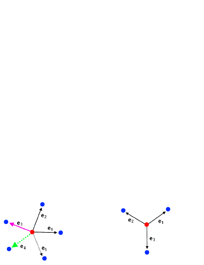
Now extending the tight binding model of 2D graphene to the 4D hyperdiamond; and using the weight vectors $\mathbf{\lambda}_{i}$ instead of $\mathbf{e}_{i}$, we can build a free fermion action on the lattice $\mathcal{H}_{4}$ by attaching a two-component left-handed spinor $\mathrm{\phi}^{a}\left(\mathbf{r}\right)$ and right-handed spinor $\mathrm{\bar{\phi}}_{\mathbf{r}}^{\dot{a}}$ to each $\mathcal{A}_{4}$-node $\mathbf{r}$, and a right-handed spinor $\mathrm{\bar{\chi}}_{\mathbf{r}+d\frac{\sqrt{5}}{2}\mathbf{\lambda}_{i}}^{\dot{a}}$ and left-handed spinor $\mathrm{\chi}_{\mathbf{r}+d\frac{\sqrt{5}}{2}\mathbf{\lambda}_{i}}^{a}$ to every $\mathcal{B}_{4}$-node at $\mathbf{r}+d\frac{\sqrt{5}}{2}\mathbf{\lambda}_{i}$. The action, describing hopping to first nearest-neighbor sites with equal probabilities in all five directions $\mathbf{\lambda}_{i}$, reads as follows:.

$\mathcal{S}_{{}_{{\small BBTW}}}$ $=$ $\mathop{\displaystyle\sum}\limits_{\mathbf{r}}\mathop{\displaystyle\sum}\limits_{i=0}^{4}\left(\mathrm{\phi}_{\mathbf{r}}\mathrm{\sigma}^{\mu}\mathrm{\bar{\chi}}_{\mathbf{r+}d\frac{\sqrt{5}}{2}\mathbf{\lambda}_{i}}-\mathrm{\chi}_{\mathbf{r}}\mathrm{\bar{\sigma}}^{\mu}\mathrm{\bar{\phi}}_{\mathbf{r-}d\frac{\sqrt{5}}{2}\mathbf{\lambda}_{i}}\right)\mathrm{\lambda}_{i}^{\mu}$ .
(4.9)

Clearly this action is invariant under the following discrete transformations

$\mathrm{\sigma}^{\mu}\mathrm{\bar{\xi}}_{\mathbf{r}\pm d\frac{\sqrt{5}}{2}\mathbf{\lambda}_{i}}$ $\longrightarrow$ $\mathrm{\sigma}^{\nu}\mathrm{\bar{\xi}}_{\mathbf{r}\pm d\frac{\sqrt{5}}{2}\mathbf{\lambda}_{j}}\left(\mathcal{O}_{ji}^{T}\right)_{\nu}^{\mu}$ , $\mathrm{\lambda}_{i}^{\mu}$ $\longrightarrow$ $\left(\mathcal{O}_{ji}\right)_{\rho}^{\mu}\mathrm{\lambda}_{j}^{\rho}.$
(4.10)

Expanding the various spinorial fields $\mathrm{\xi}_{\mathbf{r\pm v}}$ in Fourier sums as $\int\frac{d^{4}k}{\left(2\pi\right)^{4}}e^{-i\mathbf{k.r}}\left(e^{\mp i\mathbf{k.v}}\mathrm{\xi}_{\mathbf{k}}\right)$ with $\mathbf{k}$ standing for a generic wave vector in $\mathcal{H}_{4}^{\ast}$, we can put the field action $\mathcal{S}_{{}_{{\small BBTW}}}$ into the form

$\mathcal{S}_{{}_{{\small BBTW}}}$ $=$ $i\mathop{\displaystyle\sum}\limits_{\mathbf{k}}\left(\mathrm{\bar{\phi}}_{\mathbf{k}},\mathrm{\bar{\chi}}_{\mathbf{k}}\right)\left(\begin{array}[]{cc}0&-iD\\ i\bar{D}&0\end{array}\right)\left(\begin{array}[]{c}\mathrm{\phi}_{\mathbf{k}}\\ \mathrm{\chi}_{\mathbf{k}}\end{array}\right)$
(4.11)

where we have set

$D$ $=\mathop{\displaystyle\sum}\limits_{l=0}^{4}D_{l}e^{id\frac{\sqrt{5}}{2}\mathbf{k}.\mathrm{\lambda}_{l}}$ $=\mathop{\displaystyle\sum}\limits_{\mu=1}^{4}\mathrm{\sigma}^{\mu}\left(\mathop{\displaystyle\sum}\limits_{l=0}^{4}\mathrm{\lambda}_{l}^{\mu}e^{id\frac{\sqrt{5}}{2}\mathbf{k}.\mathrm{\lambda}_{l}}\right)$ ,
(4.12)

with

$D_{l}=\mathop{\displaystyle\sum}\limits_{\mu=1}^{4}\mathrm{\sigma}^{\mu}\mathrm{\lambda}_{l}^{\mu}=\left(\begin{array}[]{cc}\mathrm{\lambda}_{l}^{3}+i\mathrm{\lambda}_{l}^{4}&\mathrm{\lambda}_{l}^{1}-i\mathrm{\lambda}_{l}^{2}\\ \mathrm{\lambda}_{l}^{1}+i\mathrm{\lambda}_{l}^{2}&\mathrm{\lambda}_{l}^{3}-i\mathrm{\lambda}_{l}^{4}\end{array}\right)$ ,
(4.13)

and $p_{l}=\mathbf{k}.\mathrm{\lambda}_{l}=\sum_{\mu}\mathbf{k}_{\mu}\mathrm{\lambda}_{l}^{\mu}$. Similarly we have

$\bar{D}$ $=\mathop{\displaystyle\sum}\limits_{l=0}^{4}\bar{D}_{l}e^{-id\frac{\sqrt{5}}{2}\mathbf{k}.\mathrm{\lambda}_{l}}$ $=\mathop{\displaystyle\sum}\limits_{\mu=1}^{4}\mathrm{\bar{\sigma}}^{\mu}\left(\mathop{\displaystyle\sum}\limits_{l=0}^{4}\mathrm{\lambda}_{l}^{\mu}e^{-id\frac{\sqrt{5}}{2}\mathbf{k}.\mathrm{\lambda}_{l}}\right)$ ,
(4.14)

We end this subsection by making 3 remarks; the first one deals with the continuous limit; the second one regards the zeros of the Dirac operator and the third concerns the link with the Creutz fermions. In the continuous limit where the lattice parameter $d\rightarrow 0$, we have

$\mathop{\displaystyle\sum}\limits_{l=0}^{4}\mathrm{\lambda}_{l}^{\mu}e^{\pm id\frac{\sqrt{5}}{2}\mathbf{k}.\mathrm{\lambda}_{l}}$ $\rightarrow$ $\left(\mathop{\displaystyle\sum}\limits_{l=0}^{4}\mathrm{\lambda}_{l}^{\mu}\right)\pm i\frac{d\sqrt{5}}{2}\left[\mathop{\displaystyle\sum}\limits_{l=0}^{4}\mathrm{\lambda}_{l}^{\mu}\left(\mathbf{k}.\mathrm{\lambda}_{l}\right)\right]+...$ .
(4.15)

Moreover, since $\sum_{l=0}^{4}\mathrm{\lambda}_{l}^{\mu}=0$ and because of the identity $\sum_{l=0}^{4}\mathrm{\lambda}_{l}^{\mu}\left(\mathbf{k}.\mathrm{\lambda}_{l}\right)=\mathbf{k}^{\mu}$ following from eqs(3.16-3.17), this limit reduces to

$\mathop{\displaystyle\sum}\limits_{l=0}^{4}\mathrm{\lambda}_{l}^{\mu}e^{\pm id\frac{\sqrt{5}}{2}\mathbf{k}.\mathrm{\lambda}_{l}}$ $\rightarrow$ $\pm i\frac{d\sqrt{5}}{2}\mathbf{k}^{\mu}+...$ .
(4.16)

So we have

$D\longrightarrow i\frac{d\sqrt{5}}{2}\mathop{\displaystyle\sum}\limits_{\mu=1}^{4}\mathrm{\sigma}^{\mu}\mathbf{k}_{\mu}$ , $\bar{D}\longrightarrow-i\frac{d\sqrt{5}}{2}\mathop{\displaystyle\sum}\limits_{\mu=1}^{4}\mathrm{\bar{\sigma}}^{\mu}\mathbf{k}_{\mu}$ .
(4.17)

The operators $D$ and $\bar{D}$ have zeros for wave vectors $\mathbf{k}$ satisfying the following constraint relation

$\mathbf{k}.\mathrm{\lambda}_{l}$ $=$ $\frac{4\pi N}{5d\sqrt{5}}$ ,
(4.18)

with $N$ an arbitrary integer. The point is that for these values, the phases $e^{id\frac{\sqrt{5}}{2}\mathbf{k}.\mathrm{\lambda}_{l}}=e^{i\mathbf{\varphi}}$ and the operators $D$ and $\bar{D}$ get reduced to

$D=$ $e^{i\mathbf{\varphi}}\mathop{\displaystyle\sum}\limits_{\mu=1}^{4}\mathrm{\sigma}^{\mu}\left(\mathop{\displaystyle\sum}\limits_{l=0}^{4}\mathrm{\lambda}_{l}^{\mu}\right)$ , $\bar{D}=$ $e^{-i\mathbf{\varphi}}\mathop{\displaystyle\sum}\limits_{\mu=1}^{4}\mathrm{\bar{\sigma}}^{\mu}\left(\mathop{\displaystyle\sum}\limits_{l=0}^{4}\mathrm{\lambda}_{l}^{\mu}\right)$
(4.19)

which vanish identically due to the property $\sum_{l=0}^{4}\mathrm{\lambda}_{l}^{\mu}=0$. Following [8, 11], the Dirac operator (4.11) in the Creutz lattice model reads as follows,

$$\left(\begin{array}[]{cc}0&z\\ z^{\ast}&0\end{array}\right)$$ (4.20)

where $z=\theta_{0}I+i\theta_{1}\mathrm{\sigma}^{1}+i\theta_{2}\mathrm{\sigma}^{2}+i\theta_{3}\mathrm{\sigma}^{3}$ with

$\theta_{1}=$ $\sin p_{1}+\sin p_{2}-\sin p_{3}-\sin p_{4}$
$\theta_{2}=$ $\sin p_{1}-\sin p_{2}-\sin p_{3}+\sin p_{4}$
$\theta_{3}=$ $\sin p_{1}-\sin p_{2}+\sin p_{3}-\sin p_{4}$
$\theta_{0}=$ $B\left(4C-\cos p_{1}-\cos p_{2}-\cos p_{3}-\cos p_{4}\right)$
(4.21)

and B and C two real parameters. In the Creutz lattice model, the zero energy states correspond to $z=0$; this leads to the constraints $\theta_{i}=0$ which are solved by taking one of the momenta as $p_{1}=p$ and the others as $p_{i}=p$ or $\pi-p$. To make contact with our construction, the analogous of eqs(4.21) are given by:

$\theta_{1}=$ $\mathrm{\lambda}_{0}^{1}e^{-id\frac{\sqrt{5}}{2}p_{0}}+\mathrm{\lambda}_{1}^{1}e^{-id\frac{\sqrt{5}}{2}p_{1}}+\mathrm{\lambda}_{2}^{1}e^{-id\frac{\sqrt{5}}{2}p_{2}}+\mathrm{\lambda}_{3}^{1}e^{-id\frac{\sqrt{5}}{2}p_{3}}+\mathrm{\lambda}_{4}^{1}e^{-id\frac{\sqrt{5}}{2}p_{4}}$
$\theta_{2}=$ $\mathrm{\lambda}_{0}^{2}e^{-id\frac{\sqrt{5}}{2}p_{0}}+\mathrm{\lambda}_{1}^{2}e^{-id\frac{\sqrt{5}}{2}p_{1}}+\mathrm{\lambda}_{2}^{2}e^{-id\frac{\sqrt{5}}{2}p_{2}}+\mathrm{\lambda}_{3}^{2}e^{-id\frac{\sqrt{5}}{2}p_{3}}+\mathrm{\lambda}_{4}^{2}e^{-id\frac{\sqrt{5}}{2}p_{4}}$
$\theta_{3}=$ $\mathrm{\lambda}_{0}^{3}e^{-id\frac{\sqrt{5}}{2}p_{0}}+\mathrm{\lambda}_{1}^{3}e^{-id\frac{\sqrt{5}}{2}p_{1}}+\mathrm{\lambda}_{2}^{3}e^{-id\frac{\sqrt{5}}{2}p_{2}}+\mathrm{\lambda}_{3}^{3}e^{-id\frac{\sqrt{5}}{2}p_{3}}+\mathrm{\lambda}_{4}^{3}e^{-id\frac{\sqrt{5}}{2}p_{4}}$
$\theta_{0}=$ $\mathrm{\lambda}_{0}^{4}e^{-id\frac{\sqrt{5}}{2}p_{0}}+\mathrm{\lambda}_{1}^{4}e^{-id\frac{\sqrt{5}}{2}p_{1}}+\mathrm{\lambda}_{2}^{4}e^{-id\frac{\sqrt{5}}{2}p_{2}}+\mathrm{\lambda}_{3}^{4}e^{-id\frac{\sqrt{5}}{2}p_{3}}+\mathrm{\lambda}_{4}^{4}e^{-id\frac{\sqrt{5}}{2}p_{4}}$
(4.22)

where $p_{l}=\mathbf{k}.\mathrm{\lambda}_{l}$. These relations are complex and are, in some sense, more general than the Creutz ones (4.21). The zeros of these solutions requires $e^{id\frac{\sqrt{5}}{2}p_{i}}=e^{i\varphi}$ $\forall$ $l=0,1,2,3,4$ as anticipated in (3.12).

5 Energy dispersion and zero modes

To get the dispersion energy relations of the 4 waves components $\mathrm{\phi}_{\mathbf{k}}^{1}$, $\mathrm{\phi}_{\mathbf{k}}^{2}$, $\mathrm{\chi}_{\mathbf{k}}^{1},$ $\mathrm{\chi}_{\mathbf{k}}^{2}$ and their corresponding 4 holes, one has to solve the eigenvalues of the Dirac operator (4.11). To that purpose, we first write the 4-dimensional wave equation as follows,

$\left(\begin{array}[]{cc}0&-iD\\ i\bar{D}&0\end{array}\right)\left(\begin{array}[]{c}\mathrm{\phi}_{\mathbf{k}}\\ \mathrm{\chi}_{\mathbf{k}}\end{array}\right)$ $=$ $E\left(\begin{array}[]{c}\mathrm{\phi}_{\mathbf{k}}\\ \mathrm{\chi}_{\mathbf{k}}\end{array}\right)$ ,
(5.1)

where $\mathrm{\phi}_{\mathbf{k}}=\left(\mathrm{\phi}_{\mathbf{k}}^{1},\mathrm{\phi}_{\mathbf{k}}^{2}\right)$, $\mathrm{\chi}_{\mathbf{k}}=\left(\mathrm{\chi}_{\mathbf{k}}^{1},\mathrm{\chi}_{\mathbf{k}}^{2}\right)$ are Weyl spinors and where the $2\times 2$ matrices $D$, $\bar{D}$ are as in eqs(4.12,4.14). Then determine the eigenstates and eigenvalues of the $2\times 2$ Dirac operator matrix by solving the following characteristic equation,

$\det\left(\begin{array}[]{cccc}-E&0&D_{11}&D_{12}\\ 0&-E&D_{21}&D_{22}\\ \bar{D}_{11}&\bar{D}_{21}&-E&0\\ \bar{D}_{12}&\bar{D}_{22}&0&-E\end{array}\right)$ $=0$
(5.2)

from which one can learn the four dispersion energy eigenvalues $E_{1}\left(\mathbf{k}\right)$, $E_{2}\left(\mathbf{k}\right)$, $E_{3}\left(\mathbf{k}\right)$, $E_{4}\left(\mathbf{k}\right)$ and therefore their zeros.

5.1 Computing the energy dispersion

An interesting way to do these calculations is to act on (5.1) once more by the Dirac operator to bring it to the following diagonal form

$\left(\begin{array}[]{cc}D\bar{D}&0\\ 0&D\bar{D}\end{array}\right)\left(\begin{array}[]{c}\mathrm{\phi}_{\mathbf{k}}\\ \mathrm{\chi}_{\mathbf{k}}\end{array}\right)$ $=$ $E^{2}\left(\begin{array}[]{c}\mathrm{\phi}_{\mathbf{k}}\\ \mathrm{\chi}_{\mathbf{k}}\end{array}\right)$ .
(5.3)

Then solve separately the eigenvalues problem of the 2-dimensional equations $D\bar{D}\mathrm{\phi}_{\mathbf{k}}=E^{2}\mathrm{\phi}_{\mathbf{k}}$ and $\bar{D}D\mathrm{\chi}_{\mathbf{k}}=E^{2}\mathrm{\chi}_{\mathbf{k}}$. To do so, it is useful to set

$u\left(\mathbf{k}\right)=\mathrm{\vartheta}^{1}+i\mathrm{\vartheta}^{2}$ , $v\left(\mathbf{k}\right)=\mathrm{\vartheta}^{3}+i\mathrm{\vartheta}^{4}$
(5.4)

with

$\mathrm{\vartheta}^{\mu}=\mathop{\displaystyle\sum}\limits_{l=0}^{4}\mathrm{\lambda}_{l}^{\mu}e^{id\frac{\sqrt{5}}{2}\mathbf{k}.\mathrm{\lambda}_{l}}$ , $\mu=1,2,3,4.$
(5.5)

Notice that in the continuous limit, we have

$\mathrm{\vartheta}^{\mu}$ $\longrightarrow$ $id\frac{\sqrt{5}}{2}\mathbf{k}^{\mu}$ ,
$u\left(\mathbf{k}\right)$ $\longrightarrow$ $id\frac{\sqrt{5}}{2}\left(\mathbf{k}^{1}+i\mathbf{k}^{2}\right)$ ,
$v\left(\mathbf{k}\right)$ $\longrightarrow$ $id\frac{\sqrt{5}}{2}\left(\mathbf{k}^{3}+i\mathbf{k}^{4}\right)$ .
(5.6)

Substituting (5.4) back into (4.12) and (4.14), we obtain the following expressions,

$D\bar{D}=\left(\begin{array}[]{cc}\left|u\right|^{2}+\left|v\right|^{2}&2\bar{u}v\\ 2u\bar{v}&\left|u\right|^{2}+\left|v\right|^{2}\end{array}\right),$
(5.7)

and

$\bar{D}D=\left(\begin{array}[]{cc}\left|u\right|^{2}+\left|v\right|^{2}&2\bar{u}\bar{v}\\ 2uv&\left|u\right|^{2}+\left|v\right|^{2}\end{array}\right).$
(5.8)

By solving the characteristic equations of these $2\times 2$ matrix operators, we get the following eigenstates $\mathrm{\phi}_{\mathbf{k}}^{a\prime}$, $\mathrm{\chi}_{\mathbf{k}}^{a\prime}$ with their corresponding eigenvalues $E_{\pm}^{2}$,

         eigenstates          eigenvalues
$\mathrm{\phi}_{\mathbf{k}}^{1\prime}=$ $\sqrt{\frac{v\bar{u}}{2\left|u\right|\left|v\right|}}\mathrm{\phi}_{\mathbf{k}}^{1}+\sqrt{\frac{u\bar{v}}{2\left|u\right|\left|v\right|}}\mathrm{\phi}_{\mathbf{k}}^{2}$ $E_{+}^{2}=\left|u\right|^{2}+\left|v\right|^{2}+2\left|u\right|\left|v\right|$
$\mathrm{\phi}_{\mathbf{k}}^{2\prime}=$ $-\sqrt{\frac{v\bar{u}}{2\left|u\right|\left|v\right|}}\mathrm{\phi}_{\mathbf{k}}^{1}+\sqrt{\frac{u\bar{v}}{2\left|u\right|\left|v\right|}}\mathrm{\phi}_{\mathbf{k}}^{2}$ $E_{-}^{2}=\left|u\right|^{2}+\left|v\right|^{2}-2\left|u\right|\left|v\right|$
(5.9)

and

         eigenstates          eigenvalues
$\mathrm{\chi}_{\mathbf{k}}^{1\prime}=$ $\sqrt{\frac{\bar{u}\bar{v}}{2\left|u\right|\left|v\right|}}\mathrm{\chi}_{\mathbf{k}}^{1}+\sqrt{\frac{uv}{2\left|u\right|\left|v\right|}}\mathrm{\chi}_{\mathbf{k}}^{2}$ $E_{+}^{2}=\left|u\right|^{2}+\left|v\right|^{2}+2\left|u\right|\left|v\right|$
$\mathrm{\chi}_{\mathbf{k}}^{2\prime}=$ $-\sqrt{\frac{\bar{u}\bar{v}}{2\left|u\right|\left|v\right|}}\mathrm{\chi}_{\mathbf{k}}^{1}+\sqrt{\frac{uv}{2\left|u\right|\left|v\right|}}\mathrm{\chi}_{\mathbf{k}}^{2}$ $E_{-}^{2}=\left|u\right|^{2}+\left|v\right|^{2}-2\left|u\right|\left|v\right|$
(5.10)

By taking square roots of $E_{\pm}^{2}$, we obtain 2 positive and 2 negative dispersion energies; these are

$E_{\pm}=+\sqrt{\left(\left|u\right|\pm\left|v\right|\right)^{2}}$
(5.11)

which correspond to particles; and

$E_{\pm}^{\ast}=-\sqrt{\left(\left|u\right|\pm\left|v\right|\right)^{2}}$
(5.12)

corresponding to the associated holes.

5.2 Determining the zeros of $E_{\pm}$ and $E_{\pm}^{\ast}$

From the above energy dispersion relations, one sees that the zero modes are of two kinds as listed here below:

zeros of both $E_{+}^{2}=0,$ $E_{-}^{2}=0$
They are given by those wave vectors $\mathbf{K}_{F}$ solving the constraint relations $u\left(\mathbf{K}_{F}\right)=v\left(\mathbf{K}_{F}\right)=0$ which can be also put in the form

$\mathrm{\lambda}_{0}^{\mu}e^{id\frac{\sqrt{5}}{2}\mathbf{K}_{F}.\mathrm{\lambda}_{0}}+\mathrm{\lambda}_{1}^{\mu}e^{id\frac{\sqrt{5}}{2}\mathbf{K}_{F}.\mathrm{\lambda}_{1}}+$
$+\mathrm{\lambda}_{2}^{\mu}e^{id\frac{\sqrt{5}}{2}\mathbf{K}_{F}.\mathrm{\lambda}_{2}}+\mathrm{\lambda}_{3}^{\mu}e^{id\frac{\sqrt{5}}{2}\mathbf{K}_{F}.\mathrm{\lambda}_{3}}+\mathrm{\lambda}_{4}^{\mu}e^{id\frac{\sqrt{5}}{2}\mathbf{K}_{F}.\mathrm{\lambda}_{4}}$ $=0$
(5.13)

for all values of $\mu=1,2,3,4$; or equivalently like

$$\begin{array}[]{cc}d\frac{\sqrt{5}}{2}\mathbf{K}_{F}.\mathrm{\lambda}_{l}&=\frac{2\pi}{5}N+2\pi N_{l}.\end{array}$$ (5.14)

The solutions of these constraint equations have been studied in section 3; they are precisely given by eqs(3.15-3.17). Now, setting $\mathbf{k}=\mathbf{K}_{F}+\mathbf{q}$ with small $q=\left\|\mathbf{q}\right\|$ and expanding $D$ and $\bar{D}$, eq(5.1) gets reduced to

$\frac{d\sqrt{5}}{2}\mathop{\displaystyle\sum}\limits_{\mu=1}^{4}\mathbf{q}_{\mu}\left(\begin{array}[]{cc}0&\mathrm{\sigma}^{\mu}\\ \mathrm{\bar{\sigma}}^{\mu}&0\end{array}\right)\left(\begin{array}[]{c}\mathrm{\phi}_{\mathbf{k}}\\ \mathrm{\chi}_{\mathbf{k}}\end{array}\right)$ $=$ $E\left(\begin{array}[]{c}\mathrm{\phi}_{\mathbf{k}}\\ \mathrm{\chi}_{\mathbf{k}}\end{array}\right)$ .
(5.15)

case $E_{-}^{2}=0$ but $E_{+}^{2}=E_{+\min}^{2}\neq 0$
These minima are given by those wave vectors $\mathbf{K=k}_{\min}$ solving the following constraint relation $\left|u\left(\mathbf{K}\right)\right|=\left|v\left(\mathbf{K}\right)\right|$ or equivalently

$\mathop{\displaystyle\sum}\limits_{m,n=0}^{4}\left(\mathrm{\lambda}_{m}^{1}+i\mathrm{\lambda}_{m}^{2}\right)\left(\mathrm{\lambda}_{n}^{1}-i\mathrm{\lambda}_{n}^{2}\right)e^{id\frac{\sqrt{5}}{2}\mathbf{K}.\mathrm{\beta}_{mn}}=$
$\mathop{\displaystyle\sum}\limits_{m,n=0}^{4}\left(\mathrm{\lambda}_{m}^{3}+i\mathrm{\lambda}_{m}^{4}\right)\left(\mathrm{\lambda}_{n}^{3}-i\mathrm{\lambda}_{n}^{4}\right)e^{id\frac{\sqrt{5}}{2}\mathbf{K}.\mathrm{\beta}_{mn}}$ .
(5.16)

Expanding this equality, we get the following condition on the wave vector,

$\mathop{\displaystyle\sum}\limits_{m,n=0}^{4}\mathcal{A}_{nm}\cos\left(d\frac{\sqrt{5}}{2}\mathbf{K}.\mathrm{\beta}_{mn}\right)\left[\tan\left(d\frac{\sqrt{5}}{2}\mathbf{K}.\mathrm{\beta}_{mn}\right)-\frac{\mathcal{B}_{nm}}{\mathcal{A}_{nm}}\right]=0$ ,
(5.17)

with

$\mathcal{A}_{nm}$ $=$ $\left(\mathrm{\lambda}_{n}^{1}\mathrm{\lambda}_{m}^{2}-\mathrm{\lambda}_{m}^{1}\mathrm{\lambda}_{n}^{2}\right)-\left(\mathrm{\lambda}_{n}^{3}\mathrm{\lambda}_{m}^{4}-\mathrm{\lambda}_{m}^{3}\mathrm{\lambda}_{n}^{4}\right)$
$\mathcal{B}_{nm}$ $=$ $\left(\mathrm{\lambda}_{m}^{1}\mathrm{\lambda}_{n}^{1}+\mathrm{\lambda}_{m}^{2}\mathrm{\lambda}_{n}^{2}\right)-\left(\mathrm{\lambda}_{m}^{3}\mathrm{\lambda}_{n}^{3}+\mathrm{\lambda}_{m}^{4}\mathrm{\lambda}_{n}^{4}\right)$
(5.18)

A possible solution is given by those wave vectors $\mathbf{K}$ obeying the relation $\mathbf{K}.\mathrm{\beta}_{mn}=\frac{2}{d\sqrt{5}}\arctan\left(\mathcal{B}_{nm}/\mathcal{A}_{nm}\right)$.

6 Re-deriving BC fermions

In this section, we give the link between the above study based on SU$\left(5\right)$ symmetry and the so called Boriçi-Creutz (BC) model having two zero modes associated with the light quarks up and down of QCD. Recall that one of the important things in lattice QCD is the need to have a fermion action with a Dirac operator $\mathcal{D}$ having two zero modes at points $K$ and $K^{\prime}$ of the reciprocal space; so that they could be interpreted as the two light quarks. From this view, one may ask222we thank the referee for pointing out this question which allowed us to exhibit the relationship between our approach and BC fermions; see [21] for explicit details. whether there exists a link between the present analysis and the BC fermions [17, 18]. In answering this question, we have found that the BC model can be indeed recovered from the analysis developed in this paper. In what follows, we give the main lines of the derivation.

6.1 More on lattice action (4.9)

One of the interesting lessons we have learnt from the analysis developed in the previous sections is that the lattice action for 4D hyperdiamond fermions may generally be written like,

$\mathcal{S}$ $\sim$ $\frac{i}{4a}\mathop{\displaystyle\sum}\limits_{\mathbf{r}}\left(\mathop{\displaystyle\sum}\limits_{l=0}^{4}\bar{\Psi}_{\mathbf{r}}\Gamma^{l}\Psi_{\mathbf{r+}a\mathbf{\lambda}_{l}}+\mathop{\displaystyle\sum}\limits_{l=0}^{4}\bar{\Psi}_{\mathbf{r}}\bar{\Gamma}^{l}\Psi_{\mathbf{r-}a\mathbf{\lambda}_{l}}\right),$
(6.1)

where $a=d\frac{\sqrt{5}}{2}$, the weight vectors $\mathbf{\lambda}_{l}$ as in eqs(2.3, 3.19) and where $\Gamma^{l}$ and their complex adjoints $\bar{\Gamma}^{l}$ are $4\times 4$ complex matrices given by linear combinations of the Dirac matrices $\mathrm{\gamma}^{\mu}$ as follows

$\Gamma^{l}=\left(\mathop{\displaystyle\sum}\limits_{\mu=1}^{4}\mathrm{\gamma}^{\mu}\mathrm{\Omega}_{\mu}^{l}\right)$ , $\bar{\Gamma}^{l}=\left(\mathop{\displaystyle\sum}\limits_{\mu=1}^{4}\mathrm{\gamma}^{\mu}\mathrm{\bar{\Omega}}_{\mu}^{l}\right)$ ,
(6.2)

with $\Omega_{\mu}^{l}$ linking the lattice euclidian space time index $\mu$ and the index $l$ of the 5-dimensional representation of the $SU\left(5\right)$ symmetry of the hyperdiamond. As such the lattice action (6.1) depends on the coefficients $\Omega_{\mu}^{l}$ capturing 20 complex numbers that form a $5\times 4$ matrix representing the bi-fundamental of $SO\left(4\right)\times SU\left(5\right)$

$$\Omega_{\mu}^{l}=\left(\begin{array}[]{ccccc}\Omega_{1}^{0}&\Omega_{1}^{1}&\Omega_{1}^{2}&\Omega_{1}^{3}&\Omega_{1}^{4}\\ \Omega_{2}^{0}&\Omega_{2}^{1}&\Omega_{2}^{2}&\Omega_{2}^{3}&\Omega_{2}^{4}\\ \Omega_{3}^{0}&\Omega_{3}^{1}&\Omega_{3}^{2}&\Omega_{3}^{3}&\Omega_{3}^{4}\\ \Omega_{4}^{0}&\Omega_{4}^{1}&\Omega_{4}^{2}&\Omega_{4}^{3}&\Omega_{4}^{4}\end{array}\right).$$ (6.3)

This rank two tensor, which we decompose as $\left(\omega_{\mu},\Omega_{\mu}^{\nu}\right)$ with $\omega_{\mu}=\Omega_{\mu}^{0}$ a complex 4 component vector and $\Omega_{\mu}^{\nu}$ a complex $4\times 4$ matrix, gives enough freedom to engineer Dirac operators with a definite number of zero modes. Below, we derive the constraint equations for the zero modes of the Dirac operator; and in next subsection we apply the analysis to the BC model.

6.1.1 Dirac operator

In the reciprocal space, the lattice action (6.1) reads as

$\mathcal{S}$ $\sim$ $\mathop{\displaystyle\sum}\limits_{\mathbf{k}}\left(\mathop{\displaystyle\sum}\limits_{\mu=1}^{4}\bar{\Psi}_{\mathbf{k}}\mathcal{D}\Psi_{\mathbf{k}}\right)$
(6.4)

with Dirac operator reading as follows

$$\mathcal{D}=\frac{i}{4a}\mathop{\displaystyle\sum}\limits_{\mu=1}^{4}\mathrm{\gamma}^{\mu}\left(D_{\mu}+\bar{D}_{\mu}\right),$$ (6.5)

and where $D_{\mu}$ and its complex adjoint $\bar{D}_{\mu}$ are given by:

$D_{\mu}=\mathop{\displaystyle\sum}\limits_{l=0}^{4}\mathrm{\Omega}_{\mu}^{l}e^{ia\mathbf{k}.\mathbf{\lambda}_{l}}$ , $\bar{D}_{\mu}=\mathop{\displaystyle\sum}\limits_{l=0}^{4}\mathrm{\bar{\Omega}}_{\mu}^{l}e^{-ia\mathbf{k}.\mathbf{\lambda}_{l}}$ .
(6.6)

These operators depend on $40=2\left(4+16\right)$ real numbers

$\omega_{\mu}=\frac{1}{2}\left(u_{\mu}+iv_{\mu}\right)$ , $\Omega_{\mu}^{\nu}=\frac{1}{2}R_{\mu}^{\nu}+\frac{i}{2}J_{\mu}^{\nu}$ ,
(6.7)

and also on the five momenta $p_{l}=\hbar k_{l}$ along the $\mathbf{\lambda}_{l}$- directions. Since $k_{l}=\mathbf{k}.\mathbf{\lambda}_{l}$ and because of SU$\left(5\right)$ symmetry we have moreover the constraint relation

$k_{0}+k_{1}+k_{2}+k_{3}+k_{4}=0,\qquad\mathop{\mathrm{m}od}\frac{2\pi}{a}$ ,
(6.8)

allowing to express one of the five $k_{l}$’s in terms of the four others. For instance, we can express $k_{0}$ as follows:

$$k_{0}=-\left(k_{1}+k_{2}+k_{3}+k_{4}\right),\qquad\mathop{\mathrm{m}od}\frac{2\pi}{a}.$$ (6.9)

The next step is to find the set of the wave vectors $k_{\mu}=\left(k_{1},k_{2},k_{3},k_{4}\right)$ that give the zeros of the Dirac operator. These zeros depend on the numbers $u_{\mu},$ $v_{\mu},$ $R_{\mu}^{\nu}$ and $J_{\mu}^{\nu}$ which can be tuned in order to get the desired number of zeros.

6.1.2 Zeros modes

The zero modes of the Dirac operator $\mathcal{D}$ given by eqs(6.5-6.6) are obtained by solving the following constraint equations

$$\mathop{\displaystyle\sum}\limits_{\mu=1}^{4}\mathop{\displaystyle\sum}\limits_{l=0}^{4}\mathrm{\gamma}^{\mu}\left(\mathrm{\Omega}_{\mu}^{l}+\mathrm{\bar{\Omega}}_{\mu}^{l}\right)\cos ak_{l}+i\mathop{\displaystyle\sum}\limits_{\mu=1}^{4}\mathop{\displaystyle\sum}\limits_{l=0}^{4}\mathrm{\gamma}^{\mu}\left(\mathrm{\Omega}_{\mu}^{l}-\mathrm{\bar{\Omega}}_{\mu}^{l}\right)\sin ak_{l}=0,$$ (6.10)

together with the constraint eq(6.8). Using the decomposition $\Omega_{\mu}^{l}=\left(\omega_{\mu},\Omega_{\mu}^{\nu}\right)$, we can decompose these constraints as follows

$$\Lambda+\mathop{\displaystyle\sum}\limits_{\mu=1}^{4}\left(\mathop{\displaystyle\sum}\limits_{\nu=1}^{4}\mathrm{\gamma}^{\mu}\left(\mathrm{\Omega}_{\mu}^{\nu}+\mathrm{\bar{\Omega}}_{\mu}^{\nu}\right)\cos ak_{\nu}+i\mathop{\displaystyle\sum}\limits_{\nu=1}^{4}\mathrm{\gamma}^{\mu}\left(\mathrm{\Omega}_{\mu}^{\nu}-\mathrm{\bar{\Omega}}_{\mu}^{\nu}\right)\sin ak_{\nu}\right)=0,$$ (6.11)

where we have set

$$\Lambda=\cos ak_{0}\mathop{\displaystyle\sum}\limits_{\mu=1}^{4}\mathrm{\gamma}^{\mu}\left(\mathrm{\omega}_{\mu}+\mathrm{\bar{\omega}}_{\mu}\right)+i\sin ak_{0}\mathop{\displaystyle\sum}\limits_{\mu=1}^{4}\mathrm{\gamma}^{\mu}\left(\mathrm{\omega}_{\mu}-\mathrm{\bar{\omega}}_{\mu}\right).$$ (6.12)

Moreover using (6.7) we can put the above constraint relations into the following equivalent form

$$\Lambda+\mathop{\displaystyle\sum}\limits_{\mu=1}^{4}\left(\mathop{\displaystyle\sum}\limits_{\nu=1}^{4}\mathrm{\gamma}^{\mu}R_{\mu}^{\nu}\cos ak_{\nu}-\mathop{\displaystyle\sum}\limits_{\nu=1}^{4}\mathrm{\gamma}^{\mu}J_{\mu}^{\nu}\sin ak_{\nu}\right)=0,$$ (6.13)

and

$$\Lambda=\cos ak_{0}\left(\mathop{\displaystyle\sum}\limits_{\mu=1}^{4}\mathrm{\gamma}^{\mu}u_{\mu}\right)-\sin ak_{0}\left(\mathop{\displaystyle\sum}\limits_{\mu=1}^{4}\mathrm{\gamma}^{\mu}v_{\mu}\right)=0,$$ (6.14)

with $k_{0}$ given by eq(6.8). Eqs(6.13-6.14) define a highly non linear system of coupled equations in the four $k_{\nu}$’s; and are difficult to solve in the generic case. To overcome this difficulty, one may deal with these equations by focusing on adequate solutions for the $k_{v}$’s; and engineer the corresponding $\Omega_{\mu}^{l}$ tensor. Below, we apply this idea to the BC model.

6.2 BC fermions

6.2.1 Deriving the model

Boriçi-Creutz model [17] is a simple lattice QCD fermions for modeling and simulating the interacting dynamics of the two light quarks up and down. The Dirac operator of this model reads in the reciprocal space as follows,

$\mathcal{D}_{BC}\text{ }\sim\text{ }\frac{i}{a}\mathop{\displaystyle\sum}\limits_{\mu=1}^{4}\mathrm{\gamma}^{\mu}\sin ak_{\mu}-\frac{i}{a}\mathop{\displaystyle\sum}\limits_{\mu=1}^{4}\mathrm{\gamma}^{\mu}\cos ak_{\mu}+\frac{i}{a}\mathop{\displaystyle\sum}\limits_{\mu=1}^{4}\Gamma\cos ak_{\mu}-\frac{2i}{a}\Gamma$ ,
(6.15)

with $\Gamma=\frac{1}{2}\left(\gamma^{1}+\gamma^{2}+\gamma^{3}+\gamma^{4}\right)$. From this expression, one can check that this operator has two zero modes given by the two following wave vectors,

$\left(1\right)$ : $\left(k_{1},k_{2},k_{3},k_{4}\right)$ $=\left(0,0,0,0\right)$ ,
$\left(2\right)$ : $\left(k_{1},k_{2},k_{3},k_{4}\right)$ $=\left(\frac{\pi}{2a},\frac{\pi}{2a},\frac{\pi}{2a},\frac{\pi}{2a}\right)$ ,
(6.16)

satisfying the remarkable property

$$k_{1}+k_{2}+k_{3}+k_{4}=\frac{2\pi}{a},\quad\mathop{\mathrm{m}od}\frac{2\pi}{a}.$$ (6.17)

Clearly the operator $\mathcal{D}_{BC}$ corresponds to a particular configuration of the complex tensor $\Omega_{\mu}^{\nu}$ and the vector $\omega_{\mu}$. To see that is indeed the case, notice first that the matrix $\Gamma$ can be conveniently rewritten as $\Gamma=\frac{1}{2}\vartheta_{\mu}\gamma^{\mu}$ with,

$\vartheta_{\mu}$ $=$ $\left(1,1,1,1\right)$ .
(6.18)

The same feature is valid for the sum $\sum_{\nu=1}^{4}\cos ak_{\nu}$ which can be also put in the form $\sum_{\nu=1}^{4}\vartheta^{\nu}\cos ak_{\nu}$. Putting these expressions back into the above $\mathcal{D}_{BC}$ relation, we get:

$$\mathcal{D}_{BC}\text{ }\sim\text{ }\frac{i}{a}\mathop{\displaystyle\sum}\limits_{\mu,\nu=1}^{4}\mathrm{\gamma}^{\mu}\delta_{\mu}^{\nu}\sin ak_{\nu}-\frac{i}{a}\mathop{\displaystyle\sum}\limits_{\mu,\nu=1}^{4}\mathrm{\gamma}^{\mu}M_{\mu}^{\nu}\cos ak_{\nu}-\frac{2i}{a}\Gamma,$$ (6.19)

with

$$M_{\mu}^{\nu}=\delta_{\mu}^{\nu}-\frac{1}{2}\vartheta_{\mu}\vartheta^{\nu}$$ (6.20)

or more explicitly,

$$M_{\mu}^{\nu}=\left(\begin{array}[]{cccc}+\frac{1}{2}&-\frac{1}{2}&-\frac{1}{2}&-\frac{1}{2}\\ -\frac{1}{2}&+\frac{1}{2}&-\frac{1}{2}&-\frac{1}{2}\\ -\frac{1}{2}&-\frac{1}{2}&+\frac{1}{2}&-\frac{1}{2}\\ -\frac{1}{2}&-\frac{1}{2}&-\frac{1}{2}&+\frac{1}{2}\end{array}\right).$$ (6.21)

Now comparing eq(6.19) with the general form of the Dirac operator of eq(6.5-6.6) which also reads like

$$\Lambda+\mathop{\displaystyle\sum}\limits_{\mu=1}^{4}\left(\mathop{\displaystyle\sum}\limits_{\nu=1}^{4}\mathrm{\gamma}^{\mu}R_{\mu}^{\nu}\cos ak_{\nu}-\mathop{\displaystyle\sum}\limits_{\nu=1}^{4}\mathrm{\gamma}^{\mu}J_{\mu}^{\nu}\sin ak_{\nu}\right)=0,$$ (6.22)

we see that $\mathcal{D}_{BC}$ can be recovered by taking,

$R_{\mu}^{\nu}=-M_{\mu}^{\nu}$ , $J_{\mu}^{\nu}=-\delta_{\mu}^{\nu}$ ,
(6.23)

and

$$\Lambda=-2\Gamma=-\left(\gamma^{1}+\gamma^{2}+\gamma^{3}+\gamma^{4}\right).$$ (6.24)

Eq(6.23) leads to $\Omega_{\mu}^{\nu}=-\frac{1}{2}\left(M_{\mu}^{\nu}+i\delta_{\mu}^{\nu}\right)$; by substituting $M_{\mu}^{\nu}$ by its expression given above, the tensor $\Omega_{\mu}^{\nu}$ reads more explicitly like

$$\Omega_{\mu}^{\nu}=-\frac{\left(1+i\right)}{2}\delta_{\mu}^{\nu}+\frac{1}{4}\vartheta_{\mu}\vartheta^{\nu}.$$ (6.25)

The second constraint relation (6.24) requires

$$\left(u_{\mu}\cos ak_{0}-v_{\mu}\sin ak_{0}\right)=-\vartheta_{\mu},$$ (6.26)

with $\vartheta_{\mu}$ as in (6.18). Moreover, using eqs(6.17,6.9), we end with

$$u_{\mu}=-\vartheta_{\mu},$$ (6.27)

and $v_{\mu}$ a free vector which, for simplicity, we set to zero. Thus the tensor $\Omega_{\mu}^{l}=\left(\omega_{\mu},\Omega_{\mu}^{\nu}\right)$ describing the BC fermions is given by

$$\Omega_{\mu}^{l}=\left(\begin{array}[]{ccccc}-\frac{1}{2}&-\frac{1+2i}{4}&\frac{1}{4}&\frac{1}{4}&\frac{1}{4}\\ -\frac{1}{2}&\frac{1}{4}&-\frac{1+2i}{4}&\frac{1}{4}&\frac{1}{4}\\ -\frac{1}{2}&\frac{1}{4}&\frac{1}{4}&-\frac{1+2i}{4}&\frac{1}{4}\\ -\frac{1}{2}&\frac{1}{4}&\frac{1}{4}&\frac{1}{4}&-\frac{1+2i}{4}\end{array}\right),$$ (6.28)

with the trace property $\sum_{l}\Omega_{\mu}^{l}=-\frac{i}{2}\vartheta_{\mu}$.

6.2.2 Symmetries

Here we want to make a comment on particular symmetries of 4D lattice QCD fermions by following the analysis of ref.[6] where the study of the renormalization of this class of models has been explicitly done. There, it has been found that the breaking of discrete symmetries, such as parity $\mathcal{P}$ : $\Psi(\vec{k},k_{4})\rightarrow$ $\mathrm{\gamma}_{4}\Psi(-\vec{k},k_{4})$ and time- reversal $\mathcal{T}$: $(\vec{k},k_{4})\rightarrow$ $\mathrm{\gamma}_{5}\mathrm{\gamma}_{4}\Psi(\vec{k},-k_{4})$, is behind the appearance of relevant dimension 3 operators $\mathcal{O}_{3}^{\left(i\right)}$ and marginal dimension 4 ones $\mathcal{O}_{4}^{\left(j\right)}$ in the analysis of the Symanzik effective theory with lagrangian $\mathcal{L}_{eff}=\frac{1}{a^{4}}\sum_{n}a^{n}\sum_{j}c_{n}^{\left(j\right)}\mathcal{O}_{n}^{\left(j\right)}$. Following the above mentioned work, one starts from the 4D lattice action,

$$\mathcal{S}\sim\frac{1}{2}\sum_{\mathbf{x}}\mathop{\displaystyle\sum}\limits_{\mu=1}^{4}\left[\Psi_{\mathbf{x}}^{+}\text{ }\boldsymbol{A}^{\mu}\text{ }\Psi_{\mathbf{x}+a\mathbf{\upsilon}_{\mu}}-\Psi_{\mathbf{x}}^{+}\text{ }\boldsymbol{\bar{A}}^{\mu}\text{ }\Psi_{\mathbf{x}-a\mathbf{\upsilon}_{\mu}}-2iBC\text{ }\Psi_{\mathbf{x}}^{+}\text{ }\mathrm{\gamma}^{4}\text{ }\Psi_{\mathbf{x}}\right].$$ (6.29)

which depends on two real parameters $B$ and $C$ that are fixed by physical requirements and symmetries. This typical action depends also on particular combinations of gamma matrices $\boldsymbol{A}^{\mu}=\sum_{\nu=1}^{4}\mathrm{\gamma}^{\nu}A_{\nu}^{\mu}$ where the coefficients $A_{\nu}^{\mu}$, given in [6], form an invertible $4\times 4$ matrix with $\det\left(A_{\nu}^{\mu}\right)=-16iB$. Notice that setting $B=1$, $C=\frac{\sqrt{2}}{2}$ one recovers the Boriçi action. By performing transformations of (6.29) using Fourier integrals to move to the reciprocal space, similarity operations to exhibit particular symmetries, expansion in powers of the lattice spacing parameter $a$ to use the Symanzik effective theory; and switching on the usual gauge interactions $\partial_{\mu}\rightarrow\mathfrak{D}_{\mu}=\partial_{\mu}-ig\mathcal{A}_{\mu}$ with field strength $\mathcal{F}_{\mu\nu}=\frac{i}{g}\left[\mathfrak{D}_{\mu},\mathfrak{D}_{\nu}\right]$, we get up to the first order in the parameter $a$ the following effective field action,

$$\mathcal{L}_{eff}=\mathop{\displaystyle\sum}\limits_{\mathbf{x}}\left[\bar{Q}\left(\gamma^{\mu}\otimes I\right)\mathfrak{D}_{\mu}Q-\frac{1}{4}\mathcal{F}_{\mu\nu}\mathcal{F}^{\mu\nu}+a\mathcal{O}_{5}+ord\left(a^{2}\right)\right],$$

with $Q_{\alpha}$ standing for the quark isodoublet $\left(u_{\alpha},d_{\alpha}\right)$ and $\mathcal{O}_{5}$ some dimension 5 operator that can be found in [6]. This effective theory has several symmetries in particular: (1) the manifest gauge invariance, (2) $U_{B}\left(1\right)$ baryon number, (3) $U_{L}\left(1\right)\times U_{R}\left(1\right)$ chiral symmetry, (4) $\mathcal{CPT}$ invariance and (5) symmetry under $S_{4}$ permutation of the four hyperplane axis corresponding to $C=BS$ with $e^{iK}=C+iS$. The authors of [6] concluded their work by two remarkable results: (i) the engineering of chirally symmetric action with minimal fermion doubling which does not generate dimension three operators $\mathcal{O}_{3}$ is possible as far as $\mathcal{PT}$ symmetry is preserved. This invariance is sufficient to forbid the relevant dimension 3 operators $\mathcal{O}_{3}^{\left(i\right)}$ whose typical forms are listed below,

broken $\mathcal{P}$ $:$ $\mathcal{O}_{3}^{\left(1\right)}=i$ $\bar{\Psi}_{\vec{k},k_{4}}\text{ }\gamma_{j}$ $\Psi_{\vec{k},k_{4}}$ , $\mathcal{O}_{3}^{\left(2\right)}=i$ $\bar{\Psi}_{\vec{k},k_{4}}\text{ }\gamma_{4}\gamma_{5}$ $\Psi_{\vec{k},k_{4}}$
broken $\mathcal{T}$ $:$ $\mathcal{O}_{3}^{\left(3\right)}=i$ $\bar{\Psi}_{\vec{k},k_{4}}\text{ }\gamma_{j}\gamma_{5}$ $\Psi_{\vec{k},k_{4}}$ , $\mathcal{O}_{3}^{\left(4\right)}=i$ $\bar{\Psi}_{\vec{k},k_{4}}$ $\gamma_{j}\gamma_{5}$ $\Psi_{\vec{k},k_{4}}$

with $\gamma_{j}$ standing for $\gamma_{1}$, $\gamma_{2}$ , $\gamma_{3}$. (ii) For particular values of parameters of the theory, there may emerge some additional non standard symmetries which could be used to eliminate the relevant operators. These results are important and may serve as guide lines in dealing with this problem by using the hyperdiamond symmetries based on roots and weights of $SU\left(5\right)$. Below, we give a comment on this matter; an exact answer needs however a deeper analysis. In the $SU\left(5\right)$ framework, the previous action (6.29) gets extended as follows

$$\mathcal{S}_{su_{5}}\sim\frac{i}{a}\mathop{\displaystyle\sum}\limits_{\mathbf{x}}\mathop{\displaystyle\sum}\limits_{\mu}\left(\mathop{\displaystyle\sum}\limits_{l=0}^{4}\left[\bar{\Psi}_{\mathbf{x}}\mathrm{\gamma}^{\mu}\mathrm{\Omega}_{\mu}^{l}\Psi_{\mathbf{x+}a\mathbf{\lambda}_{l}}+\bar{\Psi}_{\mathbf{x}}\mathrm{\gamma}^{\mu}\mathrm{\bar{\Omega}}_{\mu}^{l}\Psi_{\mathbf{x-}a\mathbf{\lambda}_{l}}\right]\right),$$ (6.30)

where $\mathrm{\Omega}_{\mu}^{l}$ as before and the $\mathbf{\lambda}_{l}$’s are the weight vectors of the 5-dimensional representation of SU$\left(5\right)$. Clearly, this lattice action is more general than eq(6.29); and has two interesting features that are useful in dealing with the study of underlying symmetries and renormalization of $\mathcal{S}_{su_{5}}$. First, the $SU\left(5\right)$ property (3.1) on the weight vectors namely $\sum_{l}\mathbf{\lambda}_{l}^{\mu}=0$ induces in turns the following constraint relation on the wave vectors $k_{\mu},$

$\mathop{\displaystyle\sum}\limits_{l=0}^{5}k_{l}=0$, with $k_{l}=\mathop{\displaystyle\sum}\limits_{\mu=1}^{5}k_{\mu}.\lambda_{l}^{\mu}$.

This constraint is invariant under $\mathcal{PT}$ symmetry acting on wave vectors as $k_{\mu}\rightarrow-k_{\mu}$; but not preserved under parity $\mathcal{P}$ nor time- reversal $\mathcal{T}$ separately. Second the generalized action $\mathcal{S}_{su_{5}}$ depends on 20 complex (40 real) moduli carried by the tensor $\mathrm{\Omega}_{\mu}^{l}$. This number gives quite enough freedom to engineer QCD-like models with two zeros for the Dirac operator as we have done in case of BC model; may lead to desired symmetries of the Symanzik effective theory that follow from the expansion of the action $\mathcal{S}_{su_{5}}$ in powers of the lattice parameter; and may allow to make appropriate choices to eliminate relevant operators. Progress in this matter will be reported in a future occasion.

7 Conclusion

In this paper, we have studied the lattice fermion action for pristine 4D hyperdiamond $\mathcal{H}_{4}$ with desired properties for 4D lattice QCD simulations. Using the $SU\left(5\right)$ hidden symmetry of $\mathcal{H}_{4}$, we have constructed a BBTW- like lattice model by mimicking 2D graphene model. To that purpose, we first studied the link between the construction of [5] and $SU\left(5\right)$; then we refined BBTW lattice action by using the weight vectors $\mathbf{\lambda}_{0},$ $\mathbf{\lambda}_{1},$ $\mathbf{\lambda}_{2},$ $\mathbf{\lambda}_{3},$ $\mathbf{\lambda}_{4}$ of the 5-dimensional representation of $SU\left(5\right)$. After that we studied explicitly the solutions of the zeros of the Dirac operator in terms of the $SU\left(5\right)$ simple roots $\mathbf{\alpha}_{1},$ $\mathbf{\alpha}_{2},$ $\mathbf{\alpha}_{3},$ $\mathbf{\alpha}_{4}$, and its fundamental weights $\mathbf{\omega}_{1},$ $\mathbf{\omega}_{2},$ $\mathbf{\omega}_{3},$ $\mathbf{\omega}_{4}$,. We have found that the zeros of the Dirac operator live at the sites $\mathbf{k=}\frac{4\pi}{d\sqrt{5}}\left(N_{1}\mathbf{\omega}_{1}+N_{2}\mathbf{\omega}_{2}+N_{3}\mathbf{\omega}_{3}+N_{4}\mathbf{\omega}_{4}\right)$ of the reciprocal lattice $\mathcal{H}_{4}^{\ast}$; with $N_{i}$ integers. In addition to their quite similar continuum limit, we have also studied the link between the Dirac operator following from our construction and the one suggested by Creutz using quaternions; the Dirac operator in our approach may be viewed as a ”complexification” of the Creutz one where the role played by the $\sin\left(p_{i}\right)$’s and the $\cos\left(p_{i}\right)$’s is now played by $e^{ip_{i}}$ as shown in eqs(4.21) and (4.22). The exact link between our approach and the Boriçi-Creutz fermions has been worked out with details in section 6; where it is shown that the BC action follows exactly from (6.1) with eqs(6.2,6.28) giving the linear combinations of the Dirac matrices of the model.
It is also interesting to notice that our approach is general; and applies straightforwardly to lattice systems in diverse dimensions. The fact that the 4D hyperdiamond is related to $SU\left(5\right)$ fundamental weights $\mathbf{\omega}_{1},$ $\mathbf{\omega}_{2},$ $\mathbf{\omega}_{3},$ $\mathbf{\omega}_{4}$, and its simple roots $\mathbf{\alpha}_{1},$ $\mathbf{\alpha}_{2},$ $\mathbf{\alpha}_{3},$ $\mathbf{\alpha}_{4}$ is not specific for 4-dimensions; it can be extended to generic dimensions D where the underlying D-dimensional hyperdiamond lattice has a hidden $SU\left(D+1\right)$ symmetry with simple roots $\mathbf{\alpha}_{1},$, $\mathbf{\alpha}_{D}$ and fundamental weights $\mathbf{\omega}_{1},\mathbf{...},$ $\mathbf{\omega}_{D}$. From this view, the 2D graphene has therefore a hidden $SU\left(3\right)$ symmetry as reported in details in [3]. Our construction applies as well to the fermion actions given in [12].

Acknowledgement :
L.B Drissi would like to thank ICTP for associate membership and E.H Saidi thanks URAC-09, CNRST.

References

  • [1] P.R Wallace, Phys Rev 71, $\left(1947\right)$, 622,
  • [2] A.H.Castro-Neto et al. Rev. Mod. Phys.81, 109 $\left(2009\right)$,
  • [3] L.B Drissi, E.H Saidi, M.Bousmina, Nucl Phys B, Vol 829, p.523-533, arXiv:1008.4470,
  • [4] Michael Creutz, JHEP 04 $\left(2008\right)$ 017,[arXiv:0712.1201],
  • [5] P.F Bedaque, M.I Buchoff, B.C Tiburzi, A.Walker-Loud, Phys. Rev. D78 (2008) 017502,[arXiv:0804.1145],
  • [6] P.F.Bedaque, M.I.Buchoff, B.C.Tiburzi, A.Walker-Loud, Phys. Lett. B662 $\left(2008\right)$ 449, [arXiv:0801.3361],
  • [7] Taro Kimura, Tatsuhiro Misumi, Prog.Theor.Phys.123: 63-78, $\left(2010\right)$, arXiv:0907.3774,
  • [8] Michael Creutz, Tatsuhiro Misumi, Classification of Minimally Doubled Fermions, Phys.Rev.D82:074502,2010, arXiv:1007.3328,
  • [9] Simon Catterall, David B. Kaplan, Mithat Unsal, Exact lattice supersymmetry, arXiv:0903.4881, To be published in Physics Reports,
  • [10] Simon Catterall, Eric Dzienkowski, Joel Giedt, Anosh Joseph, Robert Wells, Perturbative renormalization of lattice N=4 super Yang-Mills theory, arXiv:1102.1725,
  • [11] A.Borici, Phys. Rev. D78 $\left(2008\right)$ 074504, [arXiv:0712.4401],
  • [12] Taro Kimura, Tatsuhiro Misumi, Prog.Theor.Phys.123, 63, $\left(2010\right)$, arXiv:0907.3774,
  • [13] T. Kimura and T. Misumi, Prog.Theor.Phys.124: 415-432, $\left(2010\right)$, arXiv:0907.1371.
  • [14] J.B Kogut, L. Susskind, Phys Rev D11, 395, $\left(1975\right),$
  • [15] H.B Nielson, M. Ninomiya, Nucl Phys B185, $\left(1980\right)$, 20, B195,$\left(1982\right)$ 541,
  • [16] L.B Drissi, E.H Saidi, M. Bousmina, J. Math. Phys. 52, 022306 (2011), arXiv:1101.1061,
  • [17] S.Capitani, J.Weber, H.Wittig, Phys.Lett.B 681, 2009, 105, arXiv:0907.2825,
  • [18] S. Capitani, M. Creutz, J. Weber, H.Wittig, JHEP 1009:027,2010, arXiv:1006.2009,
  • [19] L.H. Karsten, Phys. Lett. B104 (1981) 315,
  • [20] F. Wilczek, Phys. Rev. Lett. 59 (1987) 2397,
  • [21] L.B Drissi, E.H Saidi, On Dirac Zero Modes in Hyperdiamond Model, arXiv:1103.1316, To appear in Phys Rev D (2011).