Abstract

On the basis of the so-called “yukawaon” model, we found out a special form of the neutrino mass matrix $M_{\nu}$ which gives reasonable predictions. The $M_{\nu}$ is given by a multiplication form made of charged lepton mass matrix $M_{e}$ and up-quark mass matrix $M_{u}$. This $M_{\nu}$ has no adjustable parameters except for those in $M_{e}$ and $M_{u}$. Here, $M_{e}$ and $M_{u}$ are described by one parameter $a_{e}$ (real) and two parameters $a_{u}$ (complex), respectively, and those parameters are constrained by their observed mass ratios. With this form of $M_{\nu}$, in spite of having only three parameters, the $M_{\nu}$ can give reasonable predictions $\sin^{2}2\theta_{atm}\simeq 0.99$, $\sin^{2}2\theta_{13}\simeq 0.015$, $\Delta m^{2}_{21}/\Delta m^{2}_{32}\simeq 0.030$, $\langle m_{ee}\rangle\simeq 0.0039$ eV, and so on, by using observed values of $m_{e}/m_{\mu}$, $m_{\mu}/m_{\tau}$, $m_{c}/m_{t}$, and $\sin^{2}\theta_{solar}$ as input values.

OU-HET-711/2011, MISC-2011-11

PACS numbers: 14.60.Pq, 11.30.Hv, 12.60.-i,

1 Introduction

The observed masses and mixings of the quarks and leptons will provide a promising clue to a unified understanding of those fundamental particles. For such the purpose, not only investigating a theoretical model, but also searching for phenomenological mass matrix seem to be still effective. As one of phenomenological mass matrix models of the quarks and leptons, the so-called “yukawaon” model [1] (a kind of “flavon” models [2]) has been proposed. Here, the “effective” Yukawa coupling constants $Y_{f}^{eff}$ are given by

$$(Y_{f}^{eff})_{ij}=\frac{y_{f}}{\Lambda}\langle(Y_{f})_{ij}\rangle\ \ \ \ \ (i,j=1,2,3),$$

$\Lambda$ is an energy scale of the effective theory, and $\langle Y_{f}\rangle$ are vacuum expectation value (VEV) matrices of scalar fields $Y_{f}$ with $3\times 3$ components. (Hereafter we call fields $Y_{f}$ “yukawaons”.) The most characteristic point in the yukawaon model is that all VEVs $\langle Y_{f}\rangle$ are described in terms of only one fundamental VEV matrix $\langle\Phi_{e}\rangle\propto{\rm diag}(\sqrt{m_{e}},\sqrt{m_{\mu}},\sqrt{m_{\tau}})$. For example, in a yukawaon model with an O(3) family symmetry [3, 4], the charged lepton, neutrino, up-quark, and down-quark mass matrices $M_{e}$, $M_{\nu}$, $M_{u}$ and $M_{d}$ are given by

$$M_{e}\propto\langle Y_{e}\rangle\propto\langle\Phi_{e}\rangle\langle\Phi_{e}\rangle,$$

$$M_{\nu}=m_{D}M_{R}^{-1}m_{D}^{T},$$

$$m_{D}\propto\langle Y_{e}\rangle,\ \ \ \ M_{R}\propto\langle Y_{R}\rangle+m_{0\nu}^{-1}\langle Y_{e}\rangle\langle Y_{e}\rangle,$$

$$\langle Y_{R}\rangle\propto\langle\Phi_{u}\rangle\langle P_{u}\rangle\langle Y_{e}\rangle+\langle Y_{e}\rangle\langle P_{u}\rangle\langle\Phi_{u}\rangle+\xi_{\nu}\left(\langle\Phi_{u}\rangle\langle P_{u}\rangle\langle Y_{e}\rangle+\langle Y_{e}\rangle\langle P_{u}\rangle\langle\Phi_{u}\rangle\right).$$

$$M_{u}\propto\langle Y_{u}\rangle\propto\langle\Phi_{u}\rangle\langle\Phi_{u}\rangle,$$

$$\langle\Phi_{u}\rangle\propto\langle\Phi_{e}\rangle(\langle E\rangle+a_{u}\langle X\rangle)\langle\Phi_{e}\rangle,$$

$$M_{d}\propto\langle Y_{d}\rangle\propto\langle\Phi_{e}\rangle(\langle E\rangle+a_{d}\langle X\rangle)\langle\Phi_{e}\rangle,$$

where

$$\langle E\rangle=v_{E}{\bf 1}=v_{E}\left(\begin{array}[]{ccc}1&0&0\\ 0&1&0\\ 0&0&1\end{array}\right),\ \ \ \langle X\rangle=v_{X}S_{3}\equiv\frac{1}{3}v_{X}\left(\begin{array}[]{ccc}1&1&1\\ 1&1&1\\ 1&1&1\end{array}\right),$$

in the diagonal basis of $M_{e}$, while $\langle P_{u}\rangle$ is given by a form

$$\langle P_{u}\rangle_{u}\propto\left(\begin{array}[]{ccc}1&0&0\\ 0&-1&0\\ 0&0&1\end{array}\right),$$

in the diagonal basis of $M_{u}$.

In this paper, we will find out a special form of the neutrino mass matrix which is compatible with the observed neutrino data in spite of having no adjustable parameters. The form will be obtained along the lines of the yukawaon model by changing the structure of $\langle Y_{e}\rangle$ from Eq.(1.2).

The neutrino mass matrix is still given by the form of seesaw type, $M_{\nu}=m_{D}M_{R}^{-1}m_{D}^{T}$ with $m_{D}\propto\langle Y_{e}\rangle$, but the Majorana neutrino mass matrix $M_{R}$ is changed into a simple form

$$M_{R}\propto\langle Y_{R}\rangle\propto\langle\Phi_{u}\rangle\langle Y_{e}\rangle+\langle Y_{e}\rangle\langle\Phi_{u}\rangle.$$

Here, we assume that the charged lepton mass matrix $M_{e}$ is given by

$$\langle{Y}_{e}\rangle\propto\langle\bar{\Phi}_{0}\rangle(\langle E^{\prime}\rangle+a_{e}\langle X_{2}\rangle)\langle\bar{\Phi}_{0}\rangle,$$

differently from Eq.(1.2), and we also redefine $\langle\Phi_{u}\rangle$ as

$$\langle\Phi_{u}\rangle\propto\langle\Phi_{0}\rangle(\langle E\rangle+a_{u}\langle X_{3}\rangle)\langle\Phi_{0}\rangle,$$

where $\langle E^{\prime}\rangle=\langle E\rangle=v_{E}{\bf 1}$ and

$$\langle X_{2}\rangle=v_{X}S_{2}\equiv\frac{1}{2}v_{X}\left(\begin{array}[]{ccc}1&1&0\\ 1&1&0\\ 0&0&0\end{array}\right),\ \ \ \langle X_{3}\rangle=v_{X}S_{3}\equiv\frac{1}{3}v_{X}\left(\begin{array}[]{ccc}1&1&1\\ 1&1&1\\ 1&1&1\end{array}\right),$$

Note that there are no $\xi_{\nu}$ term, no $m_{0\nu}^{-1}$ term and no $\langle P_{u}\rangle$ in Eq.(1.11), i.e. $M_{\nu}$ is simply given by

$$M_{\nu}\simeq k_{\nu}\left(M_{e}^{-1}M_{u}^{1/2}+M_{u}^{1/2}M_{e}^{-1}\right).$$

In other words, there is no adjustable parameter in the present neutrino mass matrix, except for $a_{e}$ in $M_{e}$ and $a_{u}$ in $M_{u}^{12}$ (i.e. $\langle\Phi_{u}\rangle$). The purpose of the present paper is not to derive the mass matrix forms (1.11) - (1.13) theoretically, but to demonstrate that the phenomenological neutrino mass matrix (1.15) with Eqs.(1.11) - (1.13) can be compatible with the present neutrino data in spite of quite few parameters. We predict $\sin^{2}2\theta_{atm}\simeq 0.99$, $\sin^{2}2\theta_{13}\simeq 0.015$, $\Delta m^{2}_{21}/\Delta m^{2}_{32}\simeq 0.030$, $\langle m_{ee}\rangle\simeq 0.0039$ eV, and so on, by using observed values of $m_{e}/m_{\mu}$, $m_{\mu}/m_{\tau}$, and $\sin^{2}\theta_{solar}$ as input values. In this paper, for simplicity, we do not discuss the down-quark mass matrix $M_{d}$ and the Cabibbo-Maskawa- Kobayashi [5] (CKM) mixing.

In the next section, superpotentials for yukawaons and the assignments of the fields in the present U(3) yukawaon model are investigated. In Sec. 3, numerical results of the model are discussed. Sec. 4 is devoted to the concluding remarks. In Appendix A, $R$-charge assignments are discussed. In Appendix B, we present a rotation matrix which transforms $\langle X_{3}\rangle$ into $\langle X_{2}\rangle$.

2 Superpotential

In this section, we give superpotentials for the yukawaons and the assignments of the fields in the present U(3) yukawaon model.

In the yukawaon model, the order of the fields is important. Therefore, in this paper, let us assume a U(3) family symmetry instead of O(3) and denote fields ${\bf 6}^{*}$ and ${\bf 6}$ of U(3) as $\bar{A}$ and $A$, respectively. (Therefore, it should be noted that a term $\bar{A}B\bar{C}$ is allowed, but $\bar{A}\bar{C}B$ and $B\bar{A}\bar{C}$ are forbidden.) In the U(3) model, for example, the relation (1.6) is re-expressed as

$$(M_{u})^{ij}\propto\langle\bar{Y}_{u}^{ij}\rangle\propto\langle\bar{\Phi}_{u}^{ik}\rangle\langle{E}^{u}_{kl}\rangle\langle\bar{\Phi}_{u}^{lj}\rangle,$$

with $\langle{E}^{u}\rangle={v}_{E}{\bf 1}$. In order to distinguish each yukawaon from other yukawaons, although we assumed U(1)_X charge in the O(3) model [3, 4], in this U(3) model, we assume only $R$ charge conservation instead of U(1)_X charge conservation. For the right handed neutrino sector ($\bar{Y}_{R}$), it should be noted that we cannot add $\bar{Y_{e}}\bar{Y}_{e}$ term to $\bar{Y}_{R}$ as in Eq.(1.4). In the old model, we assigned the U(1)_X charges $Q_{X}$ only for gauge singlet fields, e.g. $Q_{X}(\ell)=Q_{X}(H_{d})$, i.e. $Q_{X}(Y_{e})=-Q(e^{c})$. Besides, we assumed $Q_{X}(e^{c})=Q(\nu^{c})$ in order to build a model without $Y_{\nu}$. Therefore, we could obtain $Q_{X}(Y_{R})=Q_{X}(Y_{e}Y_{e})$ in the old model. However, in this U(3) model, we cannot obtain $R(Y_{R})=R(\bar{Y}_{e}E\bar{Y}_{e})$. Besides, we cannot introduce a $\xi_{\nu}$ term such as in Eq.(1.5).

We assume the following superpotential $W=W_{Y}+W_{e}+W_{d}+W^{\prime}_{u}+W_{u}+W_{R}+W_{E}$:

$$W_{Y}=\frac{y_{e}}{\Lambda}{\ell}_{i}\bar{Y}_{e}^{ij}e^{c}_{j}H_{d}+\frac{y_{\nu}}{\Lambda}{\ell}_{i}\bar{Y}_{e}^{ij}\nu^{c}_{j}H_{u}+\lambda_{R}\nu^{c}_{i}\bar{Y}_{R}^{ij}\nu^{c}_{j}$$

$$+\frac{y_{u}}{\Lambda}u^{c}_{i}\bar{Y}_{u}^{ij}q_{j}H_{u}+\frac{y_{d}}{\Lambda}d^{c}_{i}\bar{Y}_{d}^{ij}q_{j}H_{d}+\mu_{H}H_{u}H_{d},$$

$$W_{e}=\mu_{e}{\rm Tr}[\bar{Y}_{e}\Theta^{e}]+\frac{\lambda_{e}}{\Lambda}{\rm Tr}[\bar{\Phi}_{0}(E^{\prime}+a_{e}X_{2})\bar{\Phi}_{0}\Theta^{e}],$$

$$W_{d}=\mu_{d}{\rm Tr}[\bar{Y}_{d}{\Theta}^{d}]+\frac{\lambda_{d}}{\Lambda}{\rm Tr}[\bar{\Phi}_{0}(E+a_{d}e^{i\alpha_{d}}X_{3})\bar{\Phi}_{0}{\Theta}^{d}],$$

$$W^{\prime}_{u}=\mu^{\prime}_{u}{\rm Tr}[\bar{\Phi}_{u}\Theta^{u\prime}]+\frac{\lambda^{\prime}_{u}}{\Lambda}{\rm Tr}[\bar{\Phi}_{0}(E+a_{u}e^{i\alpha_{u}}X_{3})\bar{\Phi}_{0}\Theta^{u\prime}],$$

$$W_{u}=\mu_{u}{\rm Tr}[\bar{Y}_{u}{\Theta}^{u}]+\frac{\lambda_{u}}{\Lambda}{\rm Tr}[\bar{\Phi}_{u}{E}^{u}\bar{\Phi}_{u}{\Theta}_{u}]+\frac{\lambda_{0u}}{\Lambda^{5}}{\rm Tr}[(\bar{E}_{u}E^{u})^{3}\bar{E}_{u}\Theta^{u}],$$

$$W_{R}=\mu_{R}{\rm Tr}[\bar{Y}_{R}{\Theta}^{R}]+\frac{\lambda_{R}}{\Lambda}{\rm Tr}[\left(\bar{\Phi}_{u}E^{u}\bar{Y}_{e}+\bar{Y}_{e}{E}^{u}\bar{\Phi}_{u}\right){\Theta}^{R}],$$

where, in Eq.(2.2), $q$ and $\ell$ are SU(2)_L doublet fields, and $f^{c}$ ($f=u,d,e,\nu$) are SU(2)_L singlet fields. The other fields in Eqs.(2.3)-(2.7) have quantum numbers defined in Table 1.

	$H_{u}$	$H_{d}$	$E^{u}$	$\bar{E}_{u}$	$\Theta_{8+1}$
U(3)	${\bf 1}$	${\bf 1}$	${\bf 6}$	${\bf 6}^{*}$	${\bf 8}+{\bf 1}$
$R$	$1$	$1$	$1-\bar{r}_{E}$	$\bar{r}_{E}$	$1$
Model	$1$	$1$	$3$	$-2$	$1$

$\ell$	$e^{c}$	$\nu^{c}$	$\bar{Y}_{e}$	$\bar{\Phi}_{0}$	$E^{\prime}$	$X^{\prime}$	$\Theta^{e}$	$\bar{Y}_{R}$	${\Theta}^{R}$
${\bf 3}$	${\bf 3}$	${\bf 3}$	${\bf 6}^{*}$	${\bf 6}^{*}$	${\bf 6}$	${\bf 6}$	${\bf 6}$	${\bf 6}^{*}$	${\bf 6}$
$r_{\ell}$	$r_{e}$	$r_{e}$	$r_{Ye}$	$r_{0}$	$r_{X^{\prime}}$	$r_{X^{\prime}}$	$2-r_{Ye}$	$r_{R}$	$2-r_{R}$
$1$	$0$	$0$	$0$	$\frac{1}{2}$	$-1$	$-1$	$2$	$2$	$0$

$q$	$u^{c}$	$d^{c}$	$\bar{Y}_{u}$	$\bar{\Phi}_{u}$	${\Theta}^{u}$	$\Theta^{u\prime}$	$\bar{Y}_{d}$	$\Theta^{d}$	$E$	$X$
${\bf 3}$	${\bf 3}$	${\bf 3}$	${\bf 6}^{*}$	${\bf 6}^{*}$	${\bf 6}$	${\bf 6}$	${\bf 6}^{*}$	${\bf 6}$	${\bf 6}$	${\bf 6}$
$r_{q}$	$r_{u}$	$r_{d}$	$r_{Yu}$	$r_{Yd}$	$2-r_{Yu}$	$2-r_{Yd}$	$r_{Yd}$	$2-r_{Yd}$	$r_{X}$	$r_{X}$
$1$	$-1$	$+1$	$+1$	$-1$	$1$	$3$	$-1$	$3$	$-2$	$-2$

Table 1: Assignments of $R$ charges, where $r_{X^{\prime}}=r_{Ye}-2r_{0}$, $r_{X}=r_{Yd}-2r_{0}$ and $R(\bar{\Phi}u)=R(\bar{Y}_{d})\equiv r_{Yd}$. The values in the third raw denote $R$ charge values in a special case under the assumptions (A.11) and (A.14). For more details, see Eqs.(A.1) - (A.20) in Appendix A.

In Eq.(2.6), the third term has been added since it has the same $R$ charge as that of $\bar{Y}_{u}\Theta^{u}$. (See Eq.(A.20) in Appendix A.) The $\lambda_{0u}$ term plays a role in shifting eigenvalues of the up-quark mass matrix $M_{u}$ by a constant value. Details of $R$ charge assignments are given in Appendix A.

For the field $E^{u}$, we assume an additional field $\bar{E}_{u}$, and consider a superpotential with a form

$$W_{E}=\lambda_{E}{\rm Tr}[E^{u}\bar{E}_{u}\Theta_{8+1}]+\lambda^{\prime}_{E}{\rm Tr}[E^{u}\bar{E}_{u}]\,{\rm Tr}[\Theta_{8+1}],$$

where $\Theta_{8+1}$ is a field ${\bf 8}+{\bf 1}$ of U(3) with $\langle\Theta_{8+1}\rangle=0$. The superpotential $W_{E}$ leads to $\langle E^{u}\rangle\langle\bar{E}_{u}\rangle\propto{\bf 1}$. We assume that the form

$$\langle\bar{E}_{u}\rangle\propto\langle E^{u}\rangle=v_{E}\,{\rm diag}(1,1,1),$$

is given by a specific form of the solutions $\langle E^{u}\rangle\langle\bar{E}_{u}\rangle\propto{\bf 1}$.

In this paper, we do not discuss a superpotential which gives the observed charged lepton mass spectrum. We only use the observed charged lepton mass values as input values in $\langle\bar{Y}_{e}\rangle_{e}$.

Under the assumption that all $\Theta$ fields take $\langle\Theta\rangle=0$, SUSY vacuum conditions lead to VEV relations from Eqs.(2.3)-(2.7). That is, instead of Eqs.(1.2) - (1.8) in the previous model, we obtain the following mass matrix relations:

$$M_{e}\propto\langle\bar{Y}_{e}\rangle\propto\langle\bar{\Phi}_{0}\rangle({\bf 1}+a_{e}S_{2})\langle\bar{\Phi}_{0}\rangle,$$

$$M_{d}\propto\langle\bar{Y}_{d}\rangle\propto\langle\bar{\Phi}_{0}\rangle({\bf 1}+a_{d}e^{i\alpha_{d}}S_{3})\langle\bar{\Phi}_{0}\rangle,$$

$$\langle\bar{\Phi}_{u}\rangle\propto\langle\bar{\Phi}_{0}\rangle({\bf 1}+a_{u}e^{i\alpha_{u}}S_{3})\langle\bar{\Phi}_{0}\rangle,$$

$$M_{u}\propto\langle\bar{Y}_{u}\rangle\propto\langle\bar{\Phi}_{u}\rangle\cdot{\bf 1}\cdot\langle\bar{\Phi}_{u}\rangle+(v_{\Phi u})^{2}\zeta_{u}{\bf 1},$$

$$M_{R}\propto\langle\bar{Y}_{R}\rangle\propto\langle\bar{\Phi}_{u}\rangle\cdot{\bf 1}\cdot\langle\bar{Y}_{e}\rangle+\langle\bar{Y}_{e}\rangle\cdot{\bf 1}\cdot\langle\bar{\Phi}_{u}\rangle.$$

Here, we can take a diagonal basis of $\langle\bar{\Phi}_{0}\rangle$ without loosing the generality:

$$\langle\bar{\Phi}_{0}\rangle={\rm diag}(v_{1},v_{2},v_{3})=v_{0}\,{\rm diag}(x_{1},x_{2},x_{3}),$$

where we have normalized $x_{i}$ as $x_{1}^{2}+x_{2}^{2}+x_{3}^{2}=1$. The neutrino mass matrix $M_{\nu}$ is given by a seesaw type $M_{\nu}=m_{D}M_{R}^{-1}m_{D}^{T}$ with $m_{D}\propto M_{e}$ similar to Eq.(1.4) [but there is no $m_{0\nu}^{-1}$]. Note that the previous relations (1.2) - (1.8) were given at a diagonal basis of the VEV $\langle\Phi_{e}\rangle$, while present relations (2.10) - (2.14) are given at a diagonal basis of the VEV $\langle\bar{\Phi}_{0}\rangle$. Here the numerical matrices $S_{3}$ and $S_{2}$ are defined by

$$S_{3}=\frac{1}{3}\left(\begin{array}[]{ccc}1&1&1\\ 1&1&1\\ 1&1&1\end{array}\right),\ \ \ \ S_{2}=\frac{1}{2}\left(\begin{array}[]{ccc}1&1&0\\ 1&1&0\\ 0&0&0\end{array}\right),$$

at the diagonal basis of the VEV $\langle\bar{\Phi}_{0}\rangle$. Note that the VEV matrix $\langle\bar{Y}_{e}\rangle$ in Eq.(2.10) is no more diagonal in this basis.

In obtaining the mixing matrices, the common coefficients are not important. Here we have taken $v_{E^{\prime}}=v_{X2}$ and $v_{E}=v_{X3}$ for simplicity. The $\zeta_{u}$ term in Eq.(2.13) comes from the new term given in Eq.(A.20). This term contributes to the up-quark mass ratios, while not to the up-quark mixing matrix, so that it does not change the predictions for the neutrino mixing parameters. We suppose that the contribution from such the higher dimensional term (A.20) is considerably small, so that it also does not visibly affect the up-quark mass ratio $m_{c}/m_{t}$, although it can slightly affect $m_{u}/m_{c}$.

3 Numerical results in the up-quark and neutrino mass matrices

In this section, we investigate whether the new VEV matrix relations (2.10) - (2.14) can well describe the observed neutrino mixing parameters together with the observed up-quark mass ratios or not.

Since the charged lepton mass matrix given by Eq.(2.10) is not diagonal, the lepton mixing matrix [Pontecorvo-Maki-Nakagawa-Sakata (PMNS) [7] mixing matrix] $U$ in the present conventions is defined by

$$U=U_{eL}^{\dagger}U_{\nu L},$$

where $U_{eL}$ and $U_{\nu L}$ are defined by

$$U_{eL}^{T}\langle\bar{Y}_{e}\rangle U_{eL}=\langle\bar{Y}_{e}\rangle^{diag}\equiv\langle\bar{Y}_{e}\rangle_{e},$$

$$U_{\nu L}^{\dagger}(M_{\nu}^{\dagger}M_{\nu})U_{\nu L}=(M_{\nu}^{\dagger}M_{\nu})^{diag},$$

and $M_{\nu}$ is given by

$$M_{\nu}=\frac{y_{\nu}^{2}}{\lambda_{R}}\left(\frac{\langle H_{u}^{0}\rangle}{\Lambda}\right)^{2}\langle\bar{Y}_{e}\rangle\langle\bar{Y}_{R}\rangle^{-1}\langle\bar{Y}_{e}\rangle.$$

Neutrino mixing parameters we discuss are $\tan^{2}\theta_{solar}=|U_{12}|^{2}/|U_{11}|^{2}$, $\sin^{2}2\theta_{atm}=4|U_{23}|^{2}|U_{33}|^{2}$, and $|U_{13}|^{2}$. Here $U_{ij}$ are the matrix elements of the lepton mixing matrix defined by (3.1).

The matrix $M_{u}$ in (2.13) is diagonalized as

$$U_{uL}^{\dagger}(M_{u}^{\dagger}M_{u})U_{uL}=(M_{u}^{\dagger}M_{u})^{diag}.$$

Here $U_{uL}$ is a mixing matrix among left-handed up-quarks $u_{Li}$ . (In the present paper, the mass matrices (i.e. $\langle\bar{Y}_{f}\rangle$) are defined by Eq.(2.2). Therefore, the conventions of the mixing matrices are somewhat changed from the conventional ones.) Note that since the VEV matrix $\langle\bar{\Phi}_{u}\rangle$ is complex and $\langle\bar{Y}_{u}\rangle$ is given by Eq.(2.13), the diagonalization of the up-quark mass matrix must be done by Eq.(3.5).

3.1  Parameters in the model

The mass matrices for quarks and neutrinos in the O(3) model have been described in terms of the fundamental VEV matrix $\langle\Phi_{e}\rangle$. On the other hand, the fundamental VEV matrix in the present model is $\langle\bar{\Phi}_{0}\rangle$ defined by Eq.(2.10) in which we have new parameter $a_{e}$. Thus the number of parameters are increased by one compared with the previous model (1.2). On the other hand, we cannot bring neither the $\xi_{\nu}$ term given in Eq.(1.5) nor $\langle P_{u}\rangle_{u}$ defined in Eq.(1.10) into the present model, so that there are no parameters which are corresponding to $\xi_{\nu}$ and $P_{u}$.

The VEV of $\langle\bar{\Phi}_{0}\rangle={\rm diag}(v_{1},v_{2},v_{3})$ is related to the charged lepton mass matrix $M_{e}$ as follows:

$$M_{e}=k\left(\begin{array}[]{ccc}\left(1+\frac{1}{2}a_{e}\right)v_{1}^{2}&\frac{1}{2}a_{e}v_{1}v_{2}&0\\ \frac{1}{2}a_{e}v_{1}v_{2}&\left(1+\frac{1}{2}a_{e}\right)v_{2}^{2}&0\\ 0&0&v_{3}^{2}\end{array}\right),$$

where $k=-(\lambda_{e}/\mu_{e}\Lambda)(y_{e}\langle H^{0}_{d}\rangle/\Lambda)v_{X^{\prime}}$, so that we obtain

$$m_{e}+m_{\mu}=k\left(1+\frac{1}{2}a_{e}\right)(v_{1}^{2}+v_{2}^{2}),$$

$$m_{e}m_{\mu}=k^{2}(1+a_{e})v_{1}^{2}v_{2}^{2},$$

and $m_{\tau}=kv_{3}^{2}$. Here, since we are interested only in the relative ratios among the eigenvalues of the charged lepton mass matrix $M_{e}$, the common coefficient $k$ is not a parameter of the model. The 3 parameters $a_{e}$, $v_{1}/v_{2}$ and $v_{2}/v_{3}$ are sufficient to determine the two charged lepton mass ratios and charged lepton mixing matrix $U_{e}$ which is described only by one parameter $\theta_{12}^{e}$. [The mixing angle $\theta^{e}_{12}$ is not observable. The observed quantities are parameters of the lepton mixing matrix defined by Eq.(3.1).] Therefore, when we give a value of the parameter $a_{e}$, the values of $v_{i}$ are completely determined by the input values of the charged lepton masses. In other words, even when we give three charged lepton masses as the inputs, one of the free parameters still remains.

Thus, in the present model, we have 4 parameters $a_{e}$, $a_{u}$, $\alpha_{u}$ and $\zeta_{u}$ (except for the input values $m_{e}$, $m_{\mu}$, and $m_{\tau}$) for the up-quark and neutrino mass matrices. On the other hand, the number of the predictable quantities are 12, i.e., 2+2+2 mass ratios (up-quark, charged lepton and neutrino mass ratios) and 4+2 PMNS mixing parameters (including two Majorana phases). At present, we know 6 observed values of $\sqrt{m_{u}/m_{c}}$, $\sqrt{m_{c}/m_{t}}$, $\tan^{2}\theta_{solar}$, $\sin^{2}2\theta_{atm}$, $\sin^{2}2\theta_{13}$, and $R_{\nu}=\Delta m^{2}_{21}/\Delta m^{2}_{32}$ in addition to the charged lepton masses.

The term $\zeta_{u}{\bf 1}$ in $M_{u}$ given in Eq.(2.13) does not affect the up-quark mixing matrix, so that it also affects neither quark or lepton mixing matrices. Since we suppose $|\zeta_{u}|^{2}\ll 1$, the term almost does not affect $\sqrt{m_{c}/m_{t}}$, although it can slightly affect $\sqrt{m_{u}/m_{c}}$. As a result, the present model predicts 11 observables by using the three parameters $(a_{e},a_{u},\alpha_{u})$. In other words, the value of $\sqrt{m_{u}/m_{c}}$ is not “ prediction”, and it is a quantity which can be adjustable by the additional parameter $\zeta_{u}$ freely.

3.2  Numerical results

Now let us show the results of numerical analysis of the model. First, we show, in Fig. 1, the $a_{u}$ dependences of the quantities $\sqrt{m_{c}/m_{t}}$, $\tan^{2}\theta_{solar}$, and $\sin^{2}2\theta_{atm}$ with taking typical values of $a_{e}=3,\ 30,\ 100$ and $\alpha_{u}=0^{\circ},\ 15^{\circ}$ in order to see rough parameter behaviors.

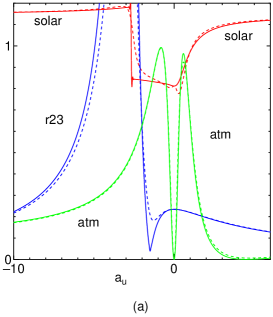
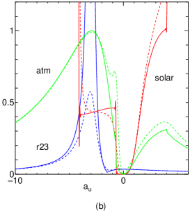
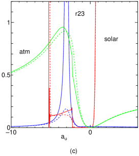
Figure 1: $\sqrt{m_{c}/m_{t}}$, $\tan^{2}\theta_{solar}$, and $\sin^{2}2\theta_{atm}$ versus a parameter $a_{u}$ for typical parameter values $a_{e}=3$ (Fig. 1 (a)), $a_{e}=30$ (Fig. 1 (b)), and $a_{e}=100$ (Fig. 1 (c)) with $\alpha_{u}=0^{\circ}$ (solid curves) and $\alpha_{u}=15^{\circ}$ (dashed curves). Curves “r23”, “solar”, and “atm” denote “r23”$=\sqrt{m_{c}/m_{t}}\times 10$, “solar”$=\tan^{2}\theta_{solar}$, and “atm”$=\sin^{2}2\theta_{atm}$, respectively.

As seen in Fig. 1, we can find that (i) the value of $\sqrt{m_{c}/m_{t}}$ takes a maximum value at $a_{u}\sim-3$ insensitively to the values of $a_{e}$ and $\alpha_{u}$; (ii) since the maximum value of $\sin^{2}2\theta_{atm}$ shows $\sin^{2}2\theta_{atm}\simeq 1$ which is in favor of the observed value, we must search for a parameter set $(a_{e},a_{u},\alpha_{u})$ which gives a maximum value of $\sin^{2}2\theta_{atm}$; (iii) a case with a small value of $a_{e}$ gives a large value of $\tan^{2}\theta_{solar}$ compared with the observed value $\tan^{2}\theta_{solar}\sim 0.5$ (see Fig. 1 (a)), so that such a case is ruled out; on the other hand, a case with a large value of $a_{e}$ gives a small $\tan^{2}\theta_{solar}$ (see Fig. 1 (c)), so that such a case is also ruled out; (iv) as a result, a region of $(a_{e},a_{u})$ which can give $\sin^{2}2\theta_{atm}\simeq 1$ and $\tan^{2}\theta_{solar}\sim 0.5$ is $(a_{e},a_{u})\sim(30,-3)$.

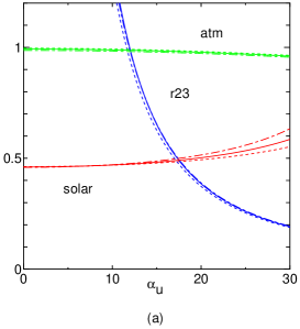
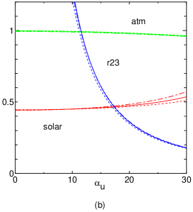
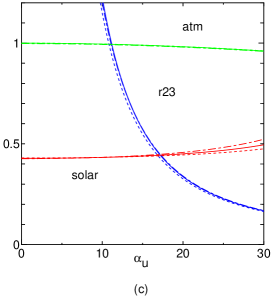
Figure 2: $\sqrt{m_{c}/m_{t}}$, $\tan^{2}\theta_{solar}$, and $\sin^{2}2\theta_{atm}$ versus a parameter $\alpha_{u}$ for typical parameter values $a_{e}=26$ (Fig. 2 (a)), $a_{e}=28$ (Fig. 2 (b)), and $a_{e}=30$ (Fig. 2 (c)) with $a_{u}=-2.9$ (dashed curves), $a_{u}=-3.0$ (solid curves), and $a_{u}=-3.1$ (dot-dashed curves). Curves “r23”, “solar”, and “atm” denote “r23”$=\sqrt{m_{c}/m_{t}}\times 10$, “solar”$=\tan^{2}\theta_{solar}$, and “atm”$=\sin^{2}2\theta_{atm}$, respectively.

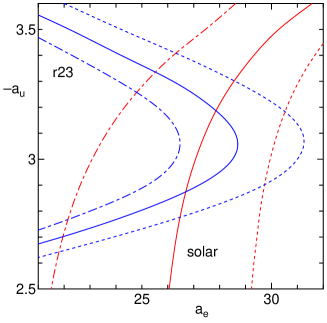
Figure 3: Contour lines of $\sqrt{m_{c}/m_{t}}$ and $\tan^{2}\theta_{solar}$ in the $(a_{e},a_{u})$ plane in the case of $\alpha_{u}=15^{\circ}$. As input values, $\sqrt{m_{c}/m_{t}}=0.0600^{+0.0045}_{-0.0047}$ and $\tan^{2}\theta_{solar}^{obs}=0.47^{+0.05}_{-0.03}$ have been used. Curves with dot-dash, solid, and dash denote the upper, center, and lower observed values, respectively. Curves “r23” and “solar” denote “r23”$=\sqrt{m_{c}/m_{t}}\times 10$ and “solar”$=\tan^{2}\theta_{solar}$, respectively.

Next, in order to determine parameter values $(a_{e},a_{u},\alpha_{u})$, let us illustrate, in Fig. 2, the $\alpha_{u}$ behaviors of $\sqrt{m_{c}/m_{t}}$, $\tan^{2}\theta_{solar}$ and $\sin^{2}2\theta_{atm}$ at $a_{e}\sim 28$ and $a_{u}\sim-3$. From Fig. 2, we search for the value $\alpha_{u}$ which gives the observed value [8] $\sqrt{m_{c}/m_{t}}=0.0600^{+0.0045}_{-0.0047}$ at $\mu=m_{Z}$. We find that the value $\alpha_{u}\simeq 15^{\circ}$ can give a reasonable fit $\sqrt{m_{c}/m_{t}}=0.0600$ insensitively to the other parameters.

Therefore, by fixing the value $\alpha_{u}=15^{\circ}$, we illustrate the contour lines of $\sqrt{m_{c}/m_{t}}$ and $\tan^{2}\theta_{solar}$ in the $(a_{e},a_{u})$ plane in Fig. 3. The curves denote $(a_{e},a_{u})$ which gives the observed values $\sqrt{m_{c}/m_{t}}=0.0600^{+0.0045}_{-0.0047}$ [8] and $\tan^{2}\theta_{solar}^{obs}=0.47^{+0.05}_{-0.03}$ [9]. As seen in Fig. 3, we have two intersection points of the curves of $\sqrt{m_{c}/m_{t}}$ and $\tan^{2}\theta_{solar}$. For the center values $\sqrt{m_{c}/m_{t}}=0.060$ and $\tan^{2}\theta_{solar}=0.47$, the solutions $(a_{e},a_{u},\alpha_{u})$ are

$$(26.7,-2.88,15^{\circ}),\ \ \ \ (27.9,-3.18,15^{\circ}).$$

We list our prediction values for these parameter solutions in Table 1. Of the two solutions obtained from the input data $\sqrt{m_{c}/m_{t}}$ and $\tan^{2}\theta_{solar}$, Table 2 suggests that we should take the former one considering the observed value of $R_{\nu}$ [9]

$$R_{\nu}\equiv\frac{\Delta m^{2}_{solar}}{\Delta m^{2}_{atm}}=(3.12^{+0.27}_{-0.23})\times 10^{-2}.$$

For reference, we also illustrate the behavior of predicted values for input values $(a_{e},a_{u},\alpha_{u})$ around the parameter solutions (3.9) in Fig. 4. As seen in Fig. 4, the predicted values $\sin^{2}2\theta_{atm}$ and $\tan^{2}\theta_{solar}$ are insensitive to the parameter values $a_{e}$, $a_{u}$, and $\alpha_{u}$ around the values $(a_{e},a_{u},\alpha_{u})=(26.7,-2.88,15^{\circ})$. However, $\sqrt{m_{c}/m_{t}}$ and $|U_{13}|^{2}$ (and also $R_{\nu}$) are somewhat dependent on these parameters. Since these parameter values are mainly obtained by taking the input value $\sqrt{m_{c}/m_{t}}=0.0600$, if the input value changes, then the predicted values will also change.

Input $(a_{e},a_{u},\alpha_{u})$	$\sqrt{m_{c}/m_{t}}$	$\tan^{2}\theta_{solar}$	$\sin^{2}2\theta_{atm}$	$\sin^{2}2\theta_{13}$	$R_{\nu}$
$(26.7,-2.88,15^{\circ})$	$0.0603$	$0.470$	$0.990$	$0.015$	$0.0303$
$(27.9,-3.18,15^{\circ})$	$0.0601$	$0.469$	$0.980$	$0.011$	$0.0204$
upper	$+0.0045$	$+0.05$			$+0.0027$
Observed value	$0.0600$	$0.47$	$>0.92$ [9]	$<0.15$ [9]	$0.0312$
lower	$-0.0047$	$-0.03$			$-0.0023$

Table 2: Predicted values for the parameter values $(a_{e},a_{u},\alpha_{u})$.

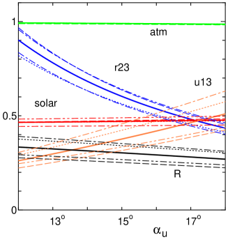
Figure 4: Predicted values versus a parameter $\alpha_{u}$ for $a_{e}=26.7$ and $a_{u}=-2.88$. Curves “r23”, “solar”, “atm”, “u13”, and “R” denote “r23”$=\sqrt{m_{c}/m_{t}}\times 10$, “solar”$=\tan^{2}\theta_{solar}$, “atm”$=\sin^{2}2\theta_{atm}$, “u13”$=|U_{13}|^{2}\times 100$, and “R”$=R_{\nu}\times 10$, respectively. For reference, curves for $(a_{e},a_{u})=(26.7,-3.00)$ (dash curve), $(26.7,-2.80)$ (dot curve), $(29,-2.88)$ (dot dash curve), and $(25,-2.88)$ (2-dot dash curve) are illustrated in addition to the curve (solid) for $(26.7,-2.88)$.

So far, we have not discussed the value of $m_{u}/m_{c}$. In the present model, the value of $m_{u}/m_{c}$ is always adjustable by the parameter $\zeta_{u}$ given in Eq.(2.13) without affecting other predicted values. In order to fit the predicted value of $\sqrt{m_{u}/m_{c}}$ to the observed value [8] $\sqrt{m_{u}/m_{c}}=0.0453^{+0.012}_{-0.010}$, we choose $\zeta_{u}$ as $\zeta_{u}=3.8\times 10^{-7}$. As seen in Table 3, the value of $\zeta_{u}$ almost does not change the numerical predictions given in Table 2.

In conclusion, we take the parameter set

$$(a_{e},a_{u},\alpha_{u},\zeta_{u})=(26.7,-2.88,15^{o},3.8\times 10^{-7}).$$

Then, we predict neutrino masses

$$m_{\nu 1}\simeq 0.012\ {\rm eV},\ \ m_{\nu 2}\simeq 0.015\ {\rm eV},\ \ m_{\nu 3}\simeq 0.051\ {\rm eV},$$

by using the input value $\Delta m^{2}_{32}\simeq 0.0024$ eV². We also predict the effective Majorana mass $\langle m_{ee}\rangle$ in the neutrinoless double beta decay [10]

$$\langle m_{ee}\rangle=\left|m_{1}U_{e1}^{2}+m_{2}U_{e2}^{2}+m_{3}U_{e3}^{2}\right|\simeq 0.0039\ {\rm eV}.$$

It is worthwhile noticing approximately degenerate neutrino masses $m_{\nu 1}\sim m_{\nu 2}$.

Input $\zeta_{u}$	$\sqrt{m_{u}/m_{c}}$	$\sqrt{m_{c}/m_{t}}$	$\tan^{2}\theta_{solar}$	$\sin^{2}2\theta_{atm}$	$\sin^{2}2\theta_{13}$	$\delta_{CP}$ ($J$)	$R_{\nu}$
$0$	$0.0180$	$0.0603$	$0.470$	$0.990$	$0.015$	$-102.5^{\circ}$ ($-0.0139$)	$0.0303$
$3.8\times 10^{-7}$	$0.0454$	$0.0602$	$0.470$	$0.990$	$0.015$	$-102.5^{\circ}$ ($-0.0139$)	$0.0303$

Table 3: Predicted values versus $\zeta_{u}$ parameter. Other parameters $(a_{e},a_{u},\alpha_{u})$ have taken the same values $(26.7,-2.88,15^{\circ})$ as those in Table 2.

4 Concluding remarks

In this paper we have found out a special form of the neutrino mass matrix $M_{\nu}$ based on a yukawaon model with U(3) family symmetry, which has quite few free parameters. With this form of $M_{\nu}$, the $M_{\nu}$ can give reasonable predictions in spite of having no adjustable parameters, i.e. the $M_{\nu}$ is simply given by the form (1.15), and the mass matrices $M_{e}$ and $M_{u}$ include parameters $a_{e}$ and $a_{u}$, respectively, which are fixed by their observed mass ratios. In this yukawaon model, the yukawaon VEV matrices are described in terms of a new fundamental VEV matrix $\langle\bar{\Phi}_{0}\rangle$. For example, the yukawaon VEV matrix $\langle\bar{Y}_{e}\rangle$ for the charged leptons is given by (2.10) which has the structure of $({\bf 1}+a_{e}S_{2})$ with a new parameter $a_{e}$. This structure in $\langle\bar{Y}_{e}\rangle$ has been chosen from a phenomenological point of view and there is no reason why $\langle\bar{Y}_{e}\rangle$ takes such a form. Nevertheless if we accept the form (2.10), then we can obtain a simple form of VEV matrix $\langle\bar{Y}_{R}\rangle$ for right-handed neutrinos without introducing the somewhat strange VEV matrix $P_{u}$ and $\xi_{\nu}$ term that were introduced in the O(3) model to get the observed nearly tribimaximal neutrino mixing [11].

The new model has only four parameters $(a_{e},a_{u},\alpha_{u},\zeta_{u})$ as far as the up-quark and lepton sectors are concerned. on the other hand, we have 12 observable quantities (2 up-quark mass ratios, 4 lepton mass ratios, and 4+2 lepton mixing parameters). The parameter $\zeta_{u}$ affects only the prediction of $m_{u}/m_{c}$, so that we have fixed it by the observed value of $r^{u}_{12}=\sqrt{m_{u}/m_{c}}$. The parameter $\alpha_{u}$ is sensitive only to $m_{c}/m_{t}$, so that we have fixed by the observed value of $r^{u}_{23}=\sqrt{m_{c}/m_{t}}$ as seen in Fig. 2 (b). The parameter $a_{e}$ is determined from the cross point of the predicted values of $r^{u}_{23}$ and $\tan^{2}\theta_{solar}$ in the $a_{e}$-$a_{u}$ plane. Note that we have used only the observed values of $r^{u}_{23}$ and $\tan^{2}\theta_{solar}$ in order to fix the three parameters $(a_{e},a_{u},\alpha_{u})$. Although we have tacitly used $\sin^{2}2\theta_{atm}\sim 1$, we have not used the observed value of $\sin^{2}2\theta_{atm}$ explicitly.

On the other hand, for the remaining 2 down-quark mass ratios and 4 CKM mixing parameters, we have additional 2 parameters ($a_{d}$ and $\alpha_{d}$). Regrettably, we cannot obtain reasonable predictions with the two parameters, although we can fit the values of down-quark mass ratios and $V_{us}$. The situation is the same as in the previous O(3) model. We must introduce a phase matrix $P_{d}$ with two parameters $(\phi_{1},\phi_{2})$ and a common mass shift term $m_{0d}{\bf 1}$. Then, five parameters can fit six observables barely. Therefore, the model is not so attractive for down-quark sector. In this paper, we did not demonstrate the explicit numerical fitting for down-quark mass rations and CKM mixing parameters.

The present U(3) model have the following interesting features in the lepton sector:

(i) The model predicts $\sin^{2}2\theta_{13}\sim 0.015$. In the previous O(3) model, the predicted value of $|U_{13}|^{2}$ was invisibly small, i.e. $|U_{13}|^{2}\sim 10^{-4}$. The T2K experiment [12] put a constraint $0.03<\sin^{2}2\theta_{13}<0.28$ ($90\%$ C.L.) for $\delta_{CP}=0$ and a normal hierarchy. Our predicted value $\sin^{2}2\theta_{13}=0.015$ seems to be somewhat lower than the experimental lower bound. However, as seen in Table 3, our prediction on $\delta_{CP}$ gives $\delta_{CP}=-103^{\circ}$, which decreases the lower bound $0.03$ of the T2K result to $0.02$. Besides, the Double CHOOZ experiment [13] has reported that $\sin^{2}2\theta_{13}=0.085\pm 0.029\pm 0.042$ at $68\%$ CL. The lower value is $\sin^{2}2\theta_{13}=0.014$. Therefore, we consider that the predicted value $\sin^{2}2\theta_{13}=0.015$ is yet not ruled out, although the status is considerably severe.

(ii) It also predicts a reasonable value of $R_{\nu}\equiv\Delta m^{2}_{solar}/\Delta m^{2}_{atm}\sim 0.03$ in contrast to the case of the O(3) model in which we could not predict $R_{\nu}$. (In the previous model, the value of $R_{\nu}$ needed to adjust the additional free parameter $m_{0\nu}^{-1}$ in Eq.(1.4).)

(iii) The present model gives approximately degenerate neutrino masses $m_{\nu 1}\sim m_{\nu 2}$. The predicted value for the effective Majorana mass $\langle m_{ee}\rangle\simeq 0.0039$ eV in the neutrinoless double beta decay will be within our reach of the future experiments.

The big ansatz is the existence of the $X_{2}$ term in the charged lepton sector (1.12). At present, there is no idea on this term. Besides, it seems that the present lepton mass structure is ill matched with the charged lepton mass relation [14]

$$\frac{m_{e}+m_{\mu}+m_{\tau}}{(\sqrt{m_{e}}+\sqrt{m_{\mu}}+\sqrt{m_{\tau}})^{2}}=\frac{2}{3}.$$

The purpose in the early stage of the yukawaon model was to predict the charged lepton mass relation (4.1). The bilinear form (1.2) for the charged lepton mass matrix was indispensable to predict [15] the relation (4.1). If we adopt the present scenario, we must reconsider the origin of the charged lepton mass spectrum. However, in this paper, we do not use the relation (4.1), but only use the observed charged lepton mass values as input values. Therefore the bilinear form such as (1.2) is not necessarily required in this paper. Nevertheless, the formula (4.1) is still attractive. On the other hand, it is also attractive that we can predict 12 observables (2+2+2 lepton and up-quark mass ratios, and 4+2 PMNS mixing parameters) under 4 adjustable parameters $(a_{e},a_{u},\alpha_{u},\zeta_{u})$ if once we accept this ansatz (1.12). It is a future task how to understand the existence of $X_{2}$ term.

In conclusion, although the form $M_{\nu}$ is, at present, not one which is derived from a rigid theoretical ground, the form will offer a suggestive hint for a unification model of quark and lepton mass matrices.

Acknowledgment

One of the authors (YK) is supported by JSPS (No. 21540266).

Appendix A: $R$ charge assignments

In the present model, as well as in the O(3) model, we construct a model without introducing a yukawaon $Y_{\nu}$ by replacing $Y_{\nu}$ by $Y_{e}$. The simple way to guarantee that the yukawaon $Y_{e}$ couples not only to the charged lepton sector but also to the Dirac neutrino sector is to introduce the following $R$ charge assignment,

$$R(\nu^{c})=R(e^{c})\equiv r_{e},$$

$$R(H_{u})=R(H_{d})=1.$$

The $R$ charge of $(\bar{E}_{u}E^{u})$ is free parameter in the form (2.8). For simplicity, we take

$$R(\bar{E}_{u}E^{u})=R(\Theta_{8+1})=1.$$

Hereafter, we will denote $R(\bar{E}_{u})$ and $R(E^{u})$ as $\bar{r}_{E}$ and $1-\bar{r}_{E}$, respectively. Each yukawaon is distinguished from other yukawaons by the $R$ charges. If we define a parameter $n$ as

$$n\equiv 2[R(\bar{Y}_{R})-R(\bar{Y}_{e})],$$

then, we can express the $R$ charges of the other fields from Eq.(2.2) as follows:

$$R(\ell)=r_{e}+\frac{1}{2}(n-2),$$

$$R(\bar{Y}_{e})=\frac{1}{2}(4-n)-2r_{e},$$

$$R(\bar{Y}_{R})=2-2r_{e},$$

$$R(\bar{Y}_{u})=n-1+\bar{r}_{E},$$

$$R(\bar{Y}_{d})=\frac{1}{2}(n-2)+\bar{r}_{E},$$

$$R(u^{c})+R(q)=2-n-\bar{r}_{E},$$

$$R(d^{c})+R(q)=2-\frac{1}{2}n-\bar{r}_{E}.$$

From Eqs.(2.6) and (2.7), we obtain

$$R(\bar{Y}_{u})=2R(\bar{\Phi}_{u})+R(E^{u}),$$

$$R(\bar{Y}_{R})=R(\bar{\Phi}_{u})+R(\bar{Y}_{e})+R(E^{u}),$$

respectively. From Eqs.(A.12) and (A.13), we obtain a relation

$$R(\bar{Y}_{u})=n-R(E^{u})=n-1+\bar{r}_{E}.$$

The relation (A.14) leads to

$$R(\bar{Y}_{u}\Theta^{u})=(n-1)R(\bar{E}_{u}E^{u})+R(\bar{E}_{u}\Theta^{u}).$$

Only when the value $n$ is a positive integer, Eq.(A.15) means that an additional term

$$\frac{\lambda_{0u}}{\Lambda^{2n-1}}{\rm Tr}[(\bar{E}_{u}E^{u})^{n-1}\bar{E}\Theta^{u}],$$

can appear in the expression (2.6). Note that if $n$ is not a positive integer, the factor $(\bar{E}_{u}E^{u})^{n-1}$ does not have a physical meaning, because a term with $(E^{u})^{-1}$ cannot appear in the superpotential terms. Therefore, the $n$ defined in Eq.(A.4) is allowed only for $n=1,2,\cdots$.

As we see in Eqs.(A.5) - (A.11), these $R$ charges are described by four parameters $r_{e}$, $R(q)$, $\bar{r}_{E}$ and $n$. Therefore, in order to fix these $R$ charge values, we have to assume four constraints for these $R$ charges. On the other hand, the fields $\bar{Y}_{e}$, $\bar{Y}_{R}$, $\bar{Y}_{u}$, $\bar{Y}_{d}$, $\bar{\Phi}_{u}$, and $\bar{E}_{u}$ are gauge singlets, so that they must be distinguished only by $R$ charges. We can choose a suitable parameter set $(n,r_{e},r_{q},\bar{r}_{E})$. Here, let us demonstrate an example of $R$ charge assignments, although it is not the purpose of the present paper to give such an explicit $R$ charge assignment.

For example, we put the following working hypothesis:

$$R(\bar{Y}_{\nu})+R(\bar{Y}_{e})=0,\ \ \ R(\bar{Y}_{u})+R(\bar{Y}_{d})=0,$$

$$R(u^{c})+R(d^{c})=0,\ \ \ R(\nu^{c})+R(e^{c})=0.$$

The constraint (A.17) is an analogy that the Yukawa coupling constants in the standard model do not have $R$ charges. The constraints (A.17) and (A.18) leads to the relation $R(\ell)=R(q)=1$. Of course, since the yukawaon $\bar{Y}_{\nu}$ has been replaced by $\bar{Y}_{e}$ in the present model, the first constraint in Eq.(A.17) reads as $R(\bar{Y}_{e})=0$, and since $R(\nu^{c})=R(e^{c})$ in the model, the second constraint in Eq.(A.6) reads as $R(e^{c})=0$. Since $R(\bar{Y}_{e})$ is given by Eq.(A.7), the requirement $R(\bar{Y}_{e})=0$ together with $R(e^{c})=0$ requires $n=4$. Thus, the constraints (A.17) and (A.18) fix the parameters $(n,r_{e},r_{q},\bar{r}_{E})$ as

$$n=4,\ \ R(e^{c})=0,\ \ R(q)=1,\ \ R(\bar{E}_{u})=-2.$$

The explicit values of these $R$ values are listed in Table 1. Since the $R$ charges of $\bar{\Phi}_{0}$, $X^{\prime}$ and $X$ are still free parameters, we take $R(\bar{\Phi}_{0})=\frac{1}{2}$ for simplicity. As we see in Table 1, the fields $\bar{Y}_{e}$, $\bar{Y}_{R}$, $\bar{Y}_{u}$, $\bar{Y}_{d}$ and $\bar{E}_{u}$ can safely have different $R$ charges from each other.

Thus, the assumption can lead to plausible $R$ charge values (A.19), so that we consider that the assumption is reasonable. Now we have an additional term,

$$\frac{\lambda_{0u}}{\Lambda^{5}}{\rm Tr}[(\bar{E}_{u}E^{u})^{3}\bar{E}_{u}\Theta^{u}],$$

which should be included in $M_{u}$ given in Eq.(2.6).

Appendix B: Rotation from $S_{3}$ into $S_{2}$

We define

$$S_{3}=\frac{1}{3}\left(\begin{array}[]{ccc}1&1&1\\ 1&1&1\\ 1&1&1\end{array}\right),\ \ \ \ S_{2}=\frac{1}{2}\left(\begin{array}[]{ccc}1&1&0\\ 1&1&0\\ 0&0&0\end{array}\right),$$

which are invariant under permutation symmetries S₃ and $S_{2}$, respectively. A rotation matrix $R$ which transforms the matrix $S_{3}$ into $S_{2}$ has been discussed in Ref.[16]. The rotation matrix $R$ is given by

$$RS_{3}R^{T}=S_{2},$$

where $R$ is defined as follows:

$$R=R_{3}(-\frac{\pi}{4})\,T\,R_{3}(\theta)\,A,$$

$$R_{3}(\theta)=\left(\begin{array}[]{ccc}\cos\theta&\sin\theta&0\\ -\sin\theta&\cos\theta&0\\ 0&0&1\end{array}\right),$$

$$T=\left(\begin{array}[]{ccc}0&0&1\\ 0&1&0\\ 1&0&0\end{array}\right),$$

$$A=\left(\begin{array}[]{ccc}\frac{1}{\sqrt{2}}&-\frac{1}{\sqrt{2}}&0\\ \frac{1}{\sqrt{6}}&\frac{1}{\sqrt{6}}&-\frac{2}{\sqrt{6}}\\ \frac{1}{\sqrt{3}}&\frac{1}{\sqrt{3}}&\frac{1}{\sqrt{3}}\end{array}\right).$$

The matrix $A$ is known as a matrix which diagonalizes the matrix $S_{3}$ into

$$A\,S_{3}\,A^{T}=\left(\begin{array}[]{ccc}0&0&0\\ 0&0&0\\ 0&0&1\end{array}\right)\equiv Z_{3},$$

and also

$$TA\,S_{3}\,(TA)^{T}=\left(\begin{array}[]{ccc}1&0&0\\ 0&0&0\\ 0&0&0\end{array}\right)\equiv Z_{1}.$$

The explicit form of $R$ is given by

$$R=\left(\begin{array}[]{ccc}\frac{1}{\sqrt{6}}-\frac{c}{2\sqrt{3}}+\frac{s}{2}&\frac{1}{\sqrt{6}}-\frac{c}{2\sqrt{3}}-\frac{s}{2}&\frac{1}{\sqrt{6}}+\frac{c}{\sqrt{3}}\\ \frac{1}{\sqrt{6}}+\frac{c}{2\sqrt{3}}-\frac{s}{2}&\frac{1}{\sqrt{6}}+\frac{c}{2\sqrt{3}}+\frac{s}{2}&\frac{1}{\sqrt{6}}-\frac{c}{\sqrt{3}}\\ \frac{c}{\sqrt{2}}+\frac{s}{\sqrt{6}}&-\frac{c}{\sqrt{2}}+\frac{s}{\sqrt{6}}&-\frac{2s}{\sqrt{6}}\end{array}\right),$$

where $s=\sin\theta$ and $c=\cos\theta$.

In the expression (B.9) of $R$, when we define

$$\begin{array}[]{l}z_{1}=\frac{1}{\sqrt{6}}-\frac{c}{2\sqrt{3}}+\frac{s}{2},\\ z_{2}=\frac{1}{\sqrt{6}}-\frac{c}{2\sqrt{3}}-\frac{s}{2},\\ z_{3}=\frac{1}{\sqrt{6}}+\frac{c}{\sqrt{3}},\end{array}$$

the rotation matrix $R$ is expressed as follows:

$$R=\left(\begin{array}[]{ccc}z_{1}&z_{2}&z_{3}\\ \sqrt{\frac{2}{3}}-z_{1}&\sqrt{\frac{2}{3}}-z_{2}&\sqrt{\frac{2}{3}}-z_{3}\\ \sqrt{\frac{2}{3}}(z_{3}-z_{2})&\sqrt{\frac{2}{3}}(z_{1}-z_{3})&\sqrt{\frac{2}{3}}(z_{2}-z_{1})\end{array}\right).$$

Here, $z_{i}$ ($i=1,2,3$) satisfies

$$z_{1}^{2}+z_{2}^{2}+z_{3}^{2}=1,$$

and we can choose $z_{i}$ such as

$$z_{1}+z_{2}+z_{3}=\sqrt{\frac{3}{2}}.$$

Suggested from the charged lepton mass relation (4.1), if we choose $z_{i}$ as

$$z_{i}=\frac{\sqrt{m_{ei}}}{\sqrt{m_{e1}+m_{e2}+m_{e3}}},$$

where $(m_{e1},m_{e2},m_{e3})=(m_{e},m_{\mu},m_{\tau})$, then, the matrix $R$ satisfies

$$R\left(\begin{array}[]{c}z_{1}\\ z_{2}\\ z_{3}\end{array}\right)=\left(\begin{array}[]{c}1\\ 0\\ 0\end{array}\right).$$

Since

$$ZS_{3}Z=\frac{1}{3}\left(\begin{array}[]{ccc}z_{1}^{2}&z_{1}z_{2}&z_{1}z_{3}\\ z_{1}z_{2}&z_{2}^{2}&z_{2}z_{3}\\ z_{1}z_{3}&z_{2}z_{3}&z_{3}^{2}\end{array}\right),$$

where

$$Z=\left(\begin{array}[]{ccc}z_{1}&0&0\\ 0&z_{2}&0\\ 0&0&z_{3}\end{array}\right),$$

the following relation holds:

$$RZS_{3}ZR^{T}=\frac{1}{3}Z_{1},$$

where $Z_{1}$ is defined by Eq.(B.8). However, note that, from Eqs.(B.8) and (B.18), we cannot conclude $RZ=(1/\sqrt{3})TA$.

Thus, it seems the rotation matrix $R$ from $S_{3}$ into $S_{2}$ is deeply related to the charged lepton mass relation (4.1), but it is not clear why the form $S_{2}$ appears in the charge lepton sector. This is still an open question at present.

References

[1] Y. Koide, Phys. Rev. D 79, 033009 (2009).
[2] C. D. Froggatt and H. B. Nielsen, Nucl. Phys.
B 147, 277 (1979).
[3]
Y. Koide, Phys. Lett. B 680, 76 (2009).
[4] H. Nishiura and Y. Koide, Phys. Rev. D 83,
035010 (2011).
[5]
N. Cabibbo, Phys. Rev. Lett. 10, 531 (1963);
M. Kobayashi and T. Maskawa, Prog. Theor. Phys. 49, 652 (1973).
[6] H. Fritzsch, Phys. Lett. 73B, 317 (1978);
85B, 81 (1979); Nucl. Phys. B155, 189 (1979).
[7] B. Pontecorvo, Zh. Eksp. Teor. Fiz. 33, 549
(1957) and 34, 247 (1957);
Z. Maki, M. Nakagawa and S. Sakata, Prog. Theor. Phys. 28,
870 (1962).
[8] Z.-z. Xing, H. Zhang and S. Zhou,
Phys. Rev. D 77, 113016 (2008).
And also see, H. Fusaoka and Y. Koide, Phys. Rev.
D 57, 3986 (1998).
[9] Particle Data Group, K. Nakamura, et al.,
J. Phys. G 37, 075021 (2010).
[10] M. Doi, T. Kotani, H. Nishiura, K. Okuda, and E. Takasugi,
Phys. Lett. B103, 219 (1981) and B113, 513 (1982).
[11] P. F. Harrison, D. H. Perkins and W. G. Scott,
Phys. Lett. B 458, 79 (1999);
Phys. Lett. B 530, 167 (2002);
Z.-z. Xing, Phys. Lett. B 533, 85 (2002);
P. F. Harrison and W. G. Scott, Phys. Lett. B 535, 163 (2002);
Phys. Lett. B 557, 76 (2003);
E. Ma, Phys. Rev. Lett. 90, 221802 (2003);
C. I. Low and R. R. Volkas, Phys. Rev. D 68, 033007 (2003).
[12] K. Abe, et al. (T2K Collaboration),
Phys. Rev. Lett. 107, 041801 (2011).
[13] H. De Kerret, a talk at Low Nu, Seoul, Nov. 2011:
http://www.dchooz.org/DocDB
/0033/003393/003/DCAtLowNu11_Kerret111109_Official.pdf.
[14] Y. Koide, Lett. Nuovo Cimento 34, 201
(1982); Phys. Lett. B120, 161 (1983);
Phys. Rev. D28, 252 (1983).
[15] Y. Koide, Mod. Phys. Lett. A5, 2319 (1990).
[16] Y. Koide and H. Fusaoka, Phys.Rev. D 66,
113004 (2002).