A giant glitch in PSR J1718$-$3718

Abstract

Radio timing observations of the high-magnetic-field pulsar PSR J1718$-$3718 have shown that it suffered a large glitch with $\Delta\nu_{g}/\nu=(33.25\pm 0.01)\times 10^{-6}$ between 2007 September (MJD 54336) and 2009 January (MJD 54855). This is the largest pulsar glitch ever observed. As is common, there was a small increase in braking torque at the time of the glitch but, unlike all other pulsars, the braking torque has continued to increase over the two years since the glitch. Polarization observations show that the mean pulse profile has about 30% linear polarization with a smooth change of position angle through the pulse and give a rotation measure of $-160\pm 22$ rad m^-2. There was no detectable change in pulse profile at the time of the glitch. The timing observations also gave an improved dispersion measure of $371.1\pm 1.7$ cm^-3 pc.

1 Introduction

PSR J1718$-$3718 was discovered in the Parkes multibeam pulsar survey (PMPS) by Hobbs et al. (2004); it is distinguished by its long period, $P\sim 3.378$ s and very high period derivative, $\dot{P}\sim 1.598\times 10^{-12}$. Assuming magnetic dipole braking, these parameters imply a relatively low characteristic age $\tau_{c}\sim 34,000$ yr and a very high surface dipole magnetic field $B_{s}\sim 7.4\times 10^{13}$ G, one of the highest known for radio pulsars, putting it close to the magnetars, i.e., anomalous X-ray pulsars (AXPs), and soft gamma-ray repeaters (SGRs), on the $P-\dot{P}$ diagram. In fact, X-ray emission at a similar level to that from quiescent AXPs was detected in Chandra data from a position consistent with that of the pulsar by Kaspi & McLaughlin (2005). More recent Chandra observations have revealed that this X-ray source is pulsed at PSR J1718$-$3718’s period (Zhu et al., 2011), confirming the association. A spectral analysis showed that the X-ray emission is thermal with a black-body temperature higher than normal for rotation-powered pulsars of similar age, strengthening the arguments that PSR J1718$-$3718 is a quiescent magnetar.

Radio timing of this pulsar using the Parkes 64-m radio telescope commenced soon after the pulsar’s discovery in 1999 and continued with some gaps until 2007 September. In order to provide contemporaneous timing data for the Chandra X-ray observations reported by Zhu et al. (2011), timing observations recommenced in 2009 January. It was immediately obvious that the pulsar had suffered a massive glitch since the earlier observations. In this paper we report on the characteristics of this glitch. We also give an improved dispersion measure (DM) for the pulsar and discuss 3.1 GHz (10 cm) pulse polarization results including the pulsar’s rotation measure (RM).

2 Timing observations and analysis

Following the pulsar discovery, timing observations were made using the center beam of the 20-cm Multibeam receiver and the analogue filterbank (AFB) system used in the PMPS (Manchester et al., 2001). The AFB system has a bandwidth of 288 MHz centered at 1374 MHz and observations were typically of 10 – 20 min duration. These observations ceased in 2007 February. In 2005 December, several timing observations were made using the Parkes digital filterbank system PDFB1 with the 10-cm receiver; this receiver has a bandwidth of 1024 MHz centered at 3100 MHz. Several observations of pulsar were also made with the 20-cm system and PDFB1 between 2007 July and 2007 September. Regular 10-cm timing observations, mainly using PDFB4, commenced in 2009 January. This system gives 1024 bins across the profile and 1024 channels across the 1024 MHz bandwidth. The 20-cm PDFB1 observations were of 10 – 15 min duration and those at 10 cm of 10 min duration. All PDFB observations were preceded by a 1-min observation of a pulsed calibration signal injected into the feed which enables calibration of the system gain and phase response (see van Straten et al., 2010). Observations of Hydra A were used to place the data on a flux density scale. Data were processed using the psrchive pulsar analysis system (Hotan et al., 2004) and the timing analysis was done using Tempo2 package (Hobbs et al., 2006; Edwards et al., 2006). The Solar-System ephemeris DE405 (Standish, 1998) was used to convert pulse times of arrival (ToAs) at the Observatory to the Solar-System barycenter. There were no significant offsets between the ToAs from the different observing systems. Results are quoted in the barycentric dynamical time (TDB) system referenced to TT(TAI) and quoted uncertainties are one standard deviation. In this paper, we discuss data up to 2011 March 28.

Figure 1 shows the variations in pulse frequency $\nu=P^{-1}$ and frequency derivative $\dot{\nu}$ through the observed data span, obtained from independent fits to short sections of data. The top panel clearly shows the large step in $\nu$ resulting from the glitch (the approximate glitch epoch is indicated by the vertical dashed line) and the middle and lower panels show that $|\dot{\nu}|$ increased significantly after the glitch. More interestingly, there appears to be a significant downward trend in the $\dot{\nu}$ values after the glitch, that is, an increase in $|\ddot{\nu}|$.

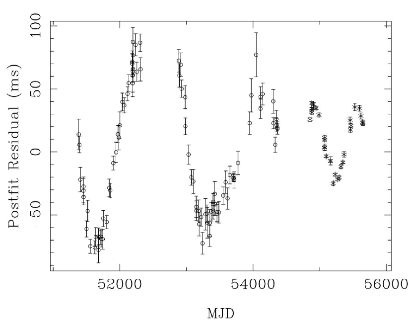
Figure 2: Timing residuals for PSR J1718$-$3718 after fitting for pulse frequency $\nu$ and its first and second time derivatives and for the jumps in these quantities at the time of the glitch using the Cholesky method. The glitch occurred in the gap between the higher-quality PDFB4 data and the earlier AFB data at about MJD 54600.

The changes in $\nu$ and its derivatives can be quantified by timing fits to the pre-glitch and post-glitch data spans; results from such fits are given in Table 1. Uncertainties ($1\sigma$) in the last quoted digit are given in parentheses. This pulsar exhibits a substantial amount of timing noise and, for both the pre-glitch and post-glitch data, the timing parameters were obtained after whitening of the post-fit residuals by fitting of high-order frequency derivatives as indicated in Table 1. A timing position was determined from the whitened pre-glitch data: RA(J2000) 17^h 18^m 09$\fs$5(6), $-37\arcdeg$ $18\arcmin$ $49\farcs 7(23)$. This position is consistent with but less precise than the Chandra X-ray position reported by Zhu et al. (2011); we therefore adopt the latter for the subsequent timing analyses. The changes in the pulse frequency and its derivatives at the time of the glitch ($\Delta\nu_{g}$, $\Delta\dot{\nu}_{g}$ and $\Delta\ddot{\nu}_{g}$) can be estimated from the pre- and post-glitch solutions. It is also possible to fit directly for them in a timing solution for the whole data span. Rather than deal with the timing noise by fitting of frequency derivatives, we have chosen to use the “Cholesky method” (Coles et al., 2011) which is implemented in Tempo2. This method explicity includes a model for the “red” timing noise and gives more realistic estimates of the parameter uncertainties. For PSR J1718$-$3718, a fit to the power spectrum of the timing residuals showed that it is well-modelled by a $f^{-3}$ power-law with a cut-off at 0.2 cycles yr^-1 and this was assumed in the Cholesky fit. Results from this fit are given in the last column of Table 1. A glitch epoch midway between the last pre-glitch and the first post-glitch ToA was assumed and its quoted uncertainty covers the gap in the data. Post-fit timing residuals are shown in Figure 2. The resulting values of $\Delta\nu_{g}$, $\Delta\dot{\nu}_{g}$ and $\Delta\ddot{\nu}_{g}$ are consistent with the differences in $\nu$, $\dot{\nu}$ and $\ddot{\nu}$ between the post-glitch and pre-glitch solutions given in Table 1 when referred to the assumed glitch epoch. Figure 2 shows that the next term in the Taylor series, $\dddot{\nu}$, appears to have changed sign from negative before the glitch to positive afterward. Further observations are required to verify that this is a glitch-related change.

Comparison of ToAs from 20-cm AFB data and 10 cm PDFB1 data recorded between 2005 June and 2006 February allowed a more accurate determination of the pulsar’s DM. To compensate for the effects of interstellar scattering, zero phase of the 20cm template profile was placed on the leading edge of the profile at about 60% of the peak amplitude, leading the peak by 0.005 in phase. The DM value resulting from the Tempo2 fit is given in Table 2.

3 Polarization observations and analysis

All post-glitch 10-cm PDFB4 observations recorded full Stokes parameter data. A total of 19 such observations were summed to give a total integration time of approximately 3.1 h. After calibration for instrumental gain and phase, the observations were summed in time and then summed in frequency with a range of rotation measures (RMs) from $-2000$ rad m^-2 to $+2000$ rad m^-2 in steps of 40 rad m^-2. A clear peak in the linearly polarized intensity $L=(Q^{2}+U^{2})^{1/2}$ was observed at about $-155$ rad m^-2. Using this RM, the data were summed to form profiles for two frequency bands. The weighted mean position angle (PA) difference between the two bands across the pulse profile and a corresponding $\Delta$RM were then computed. This process was iterated until convergence to give the final RM value given in Table 2.

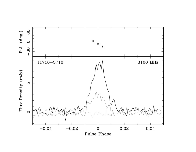
Figure 3: Polarization profiles at 10 cm (3100 MHz) for PSR J1718$-$3718. In the lower part of the figure the heavier full line is the total intensity (Stokes $I$), the lighter full line is the linearly polarized intensity ($L=(Q^{2}+U^{2})^{1/2}$) and the dotted line is the circularly polarized intensity (Stokes $V$). The upper part of the figure shows the position angle of the linearly polarized part ($\psi=0.5\tan^{-1}(U/Q)$).

The final 10-cm polarization profiles shown in Figure 3 were then formed by summing in frequency using the final RM and DM. Table 2 gives the mean flux density of the pulsed emission, the pulse width at 50% of the peak intensity and the fractional polarizations, where the $\langle\rangle$ represents a mean value over the pulse profile. Noise biases in $\langle L\rangle$ and $\langle|V|\rangle$ have been subtracted (see Yan et al., 2011). There is no evidence for any change in the 10-cm pulse profile at the time of the glitch (cf., Weltevrede et al., 2011) but, because of the low S/N ratio, a small change cannot be ruled out.

4 Discussion

The fractional pulse frequency change for this glitch, $\Delta\nu_{g}/\nu=(33.25\pm 0.01)\times 10^{-6}$, is the largest ever observed for any pulsar, magnetars included. The largest previously known was for PSR B2334+61 which had a glitch with $\Delta\nu_{g}/\nu\sim 20.5\times 10^{-6}$ in 2005 (Yuan et al., 2010a) and for magnetars, the largest glitch so far observed is for 1E 1048.1$-$5937 (PSR J1048$-$5937) with $\Delta\nu_{g}/\nu\sim 16.3\times 10^{-6}$ (Dib et al., 2009). As Figure 1 and the glitch parameters in Table 1 show, there was a step change in both $\dot{\nu}$ and $\ddot{\nu}$ at the time of the glitch. The observed value of $\Delta\dot{\nu}_{g}/\dot{\nu}\sim(6.0\pm 0.7)\times 10^{-3}$ is a little less than values typically observed in other large glitches, but certainly within the observed range (e.g., Yuan et al., 2010b; Espinoza et al., 2011).

Typically, after a large glitch, the spin-down rate relaxes back toward the pre-glitch value $\dot{\nu}_{0}$ approximately following the relation

$$\dot{\nu}(t)=\dot{\nu}_{0}(t)+\Delta\dot{\nu}_{p}+\Delta\dot{\nu}_{d}e^{-t/\tau_{d}}$$ (1)

where $\Delta\dot{\nu}_{p}$ is a quasi-permanent change to $\dot{\nu}$ at the time of the glitch and $\Delta\dot{\nu}_{d}$ is the amplitude of a component which decays away on a timescale $\tau_{d}$ (see, e.g., Yuan et al., 2010a; Espinoza et al., 2011). In some cases the $\Delta\dot{\nu}_{p}$ is not really permanent but slowly decays in an approximately linear fashion (e.g., Shemar & Lyne, 1996; Yuan et al., 2010b) and in other cases there is little or no exponential decay. If present, the exponential term implies an increase in $\ddot{\nu}$ at the time of the glitch which decays with the same time constant.

The post-glitch behaviour of PSR J1718$-$3718 was very different to the types of relaxation described above, all of which imply both $\Delta\ddot{\nu}_{g}\geq 0$ and a post-glitch value of $\ddot{\nu}\geq 0$. For PSR J1718$-$3718 there was a significant decrease in $\ddot{\nu}$ at the time of the glitch and no evidence for any exponential recovery. The step decrease in $\ddot{\nu}$ at the time of the glitch is shown by the post-glitch downward trend in $\dot{\nu}$ seen in Figure 1, by the difference in the fitted $\ddot{\nu}$ values given in Table 1 for the pre- and post-glitch data spans and by the value of $\Delta\ddot{\nu}_{g}$ from the glitch fit. It is possible that there was an exponential decay in $\dot{\nu}$ that we missed because of the large data gap around the time of the glitch but, since we see no evidence for it in the post-glitch data, its decay time constant would have to be $\stackrel{{\scriptstyle<}}{{{}_{\sim}}}250$ d. The change in $\ddot{\nu}$ has persisted for more than 700 days and seems quite distinct from the period fluctuations observed prior to the glitch (Figure 1). None of the 32 large glitch events discussed by Espinoza et al. (2011) show this type of post-glitch behaviour.

Glitches in AXPs tend to have unusual properties compared to those in normal radio pulsars (e.g., Dib et al., 2008; Livingstone et al., 2011). With its relatively long period, strong implied surface dipole magnetic field and X-ray emission, PSR J1718$-$3718 has been identified as a possible quiescent AXP (Kaspi & McLaughlin, 2005; Zhu et al., 2011). The unique post-glitch timing behaviour of this pulsar may be yet another example of these unusual properties.

The recoveries observed after most large glitches are attributed to the changing torque on the neutron-star crust as differential rotations of the internal superfluids and the crust relax back toward their equilibrium values (e.g. Alpar et al., 1993; Andersson & Comer, 2006). However in the case of PSR J1718$-$3718 we do not have a relaxation, we have the opposite — the effective braking torque increased by a small amount at the time of the glitch and has continued to increase since then. The continued increase implies a negative braking index — the post-glitch effective braking index is about $-150$ whereas before the glitch it was approximately $-15$. The characteristic timescale for the increase in torque is relatively short: $\dot{\nu}/\ddot{\nu}\sim 450$ yr.

A secular increase in the post-glitch braking torque is not predicted by standard glitch models. In the superfluid model it implies that the differential rotation of the crust and superfluid interior, decreased by the glitch, continues to decrease despite the secular slowing of the crustal rotation rate. The short characteristic timescale for the post-glitch increase in braking (or equivalently, the large negative value of the post-glitch braking index) implies that the effect is not purely electromagnetic. If the glitch resulted in, or was caused by, a crustal shift as envisaged by Ruderman (1991), then it is possible that complex interactions in the interior of the star (Ruderman et al., 1998) could result in an increasing braking torque. Another possibility is that a heat pulse associated with the glitch could result in an increasing particle flow in the magnetosphere as the surface temperature increases. Such thermal flows can have a timescale of years (Larson & Link, 2002). However Zhu et al. (2011) found no evidence for any increase in the X-ray flux associated with the glitch. Recent studies of neutron-star superfluidity (Peralta et al., 2006; Andersson et al., 2007; Link, 2011) have shown that the onset of turbulence in the interior superfluid can modify the spin behaviour of pulsars following a glitch. Specifically, the tangled vortices result in an increase in the frictional coupling between the superfluid and the rest of the star and hence a decrease in the relative velocity of the two components. If such turbulence were induced by this large glitch, then it is possible that the enhanced dissipation could further decrease the differential velocity resulting in an increasing effective braking torque.

Table 1: Timing parameters for PSR J1718$-$3718

	Pre-glitch	Post-glitch	All data
R.A. (J2000)	17h 18m 09$\fs$83	17h 18m $09\fs 83$	17h 18m $09\fs 83$
Dec. (J2000)	$-37\arcdeg$ $18\arcmin$ $51\farcs 5$	$-37\arcdeg$ $18\arcmin$ $51\farcs 5$	$-37\arcdeg$ $18\arcmin$ $51\farcs 5$
Pulse Frequency $\nu$ (Hz)	0.29600178047(8)	0.29598283922(3)	0.29599421091(13)
Freq. 1st deriv. $\dot{\nu}$ (10-15 Hz2)	$-$139.937(3)	$-$141.360(4)	$-$139.922(4)
Freq. 2nd deriv. $\ddot{\nu}$ (10-24 Hz3)	$-$1.1(3)	$-$9.86(16)	0.49(6)
Nr of frequency derivatives	8	3	2
Epoch of pulse freq. (MJD)	52874	55250	53500
Data span (MJD)	51383 – 54366	54855 – 55649	51383 – 55649
Rms timing residual (ms)	8.9	2.9	43.8
Reduced $\chi^{2}$/d.o.f.	2.3/83	4.3/26	$\cdots$
Glitch epoch (MJD)	$\cdots$	$\cdots$	54610(244)
$\Delta\nu_{g}$ (Hz)	$\cdots$	$\cdots$	$9.842(3)\times 10^{-6}$
$\Delta\dot{\nu}_{g}$ (10-15 Hz2)	$\cdots$	$\cdots$	$-0.84(9)$
$\Delta\ddot{\nu}_{g}$ (10-24 Hz3)	$\cdots$	$\cdots$	$-10.6(16)$

Table 2: Interstellar and profile parameters for PSR J1718$-$3718

Parameter	Value
Dispersion measure (cm-3 pc)	371.1(17)
Rotation Measure (rad m2)	$-$160(22)
Mean flux density at 3100 MHz $\langle I\rangle$ (mJy)	0.30
Pulse width at 50% of peak (ms)	41
Fractional linear polarization $\langle L\rangle/\langle I\rangle$ (%)	29
Fractional circular polarization $\langle V\rangle/\langle I\rangle$ (%)	5
Fractional abs. circular polarization $\langle|V|\rangle/\langle I\rangle$ (%)	7

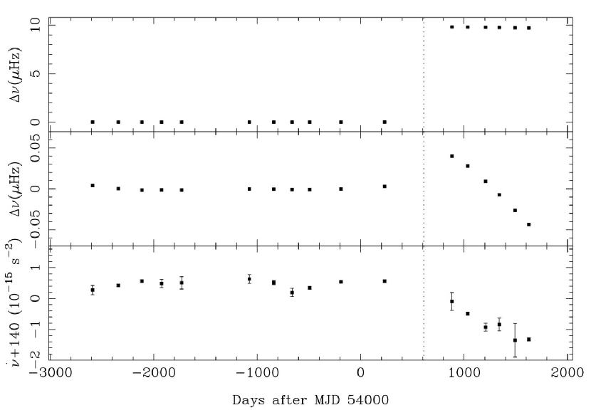
Figure 1: Variations of pulse frequency $\nu$ and frequency derivative $\dot{\nu}$ for PSR J1718$-$3718. In the middle plot, the mean post-glitch frequency has been subtracted to show more detail.

References

- Alpar et al. (1993) Alpar, M. A., Chau, H. F., Cheng, K. S., & Pines, D. 1993, ApJ, 409, 345
- Andersson & Comer (2006) Andersson, N. & Comer, G. L. 2006, Classical and Quantum Gravity, 23, 5505
- Andersson et al. (2007) Andersson, N., Sidery, T., & Comer, G. L. 2007, MNRAS, 381, 747
- Coles et al. (2011) Coles, W., Hobbs, G., Champion, D. J., Manchester, R. N., & Verbiest, J. P. W. 2011, MNRAS, submitted
- Dib et al. (2008) Dib, R., Kaspi, V. M., & Gavriil, F. P. 2008, ApJ, 673, 1044
- Dib et al. (2009) —. 2009, ApJ, 702, 614
- Edwards et al. (2006) Edwards, R. T., Hobbs, G. B., & Manchester, R. N. 2006, MNRAS, 372, 1549
- Espinoza et al. (2011) Espinoza, C. M., Lyne, A. G., Stappers, B. W., & Kramer, M. 2011, MNRAS, in press (ArXiv:1102.1743)
- Hobbs et al. (2004) Hobbs, G., Faulkner, A., Stairs, I. et al. 2004, MNRAS, 352, 1439
- Hobbs et al. (2006) Hobbs, G. B., Edwards, R. T., & Manchester, R. N. 2006, MNRAS, 369, 655
- Hotan et al. (2004) Hotan, A. W., van Straten, W., & Manchester, R. N. 2004, PASA, 21, 302
- Israel et al. (2007) Israel, G. L., Campana, S., Dall’Osso, S., Muno, M. P., Cummings, J., Perna, R., & Stella, L. 2007, ApJ, 664, 448
- Kaspi & McLaughlin (2005) Kaspi, V. M. & McLaughlin, M. A. 2005, ApJ, 618
- Larson & Link (2002) Larson, M. B. & Link, B. 2002, MNRAS, 333, 613
- Link (2011) Link, B. 2011, ArXiv:1105.4654
- Livingstone et al. (2011) Livingstone, M. A., Ng, C., Kaspi, V. M., Gavriil, F. P., & Gotthelf, E. V. 2011, ApJ, 730, 66
- Manchester et al. (2001) Manchester, R. N., Lyne, A. G., Camilo, F. et al. 2001, MNRAS, 328, 17
- Peralta et al. (2006) Peralta, C., Melatos, A., Giacobello, M., & Ooi, A. 2006, ApJ, 651, 1079
- Ruderman (1991) Ruderman, M. 1991, ApJ, 382, 587
- Ruderman et al. (1998) Ruderman, M., Zhu, T., & Chen, K. 1998, ApJ, 492, 267
- Shemar & Lyne (1996) Shemar, S. L. & Lyne, A. G. 1996, MNRAS, 282, 677
- Standish (1998) Standish, E. M. 1998, JPL Planetary and Lunar Ephemerides, DE405/LE405, Memo IOM 312.F-98-048 (Pasadena: JPL), http://ssd.jpl.nasa.gov/iau-comm4/de405iom/de405iom.pdf
- van Straten et al. (2010) van Straten, W., Manchester, R. N., Johnston, S., & Reynolds, J. E. 2010, PASA, 27, 104
- Weltevrede et al. (2011) Weltevrede, P., Johnston, S., & Espinoza, C. M. 2011, MNRAS, 411, 1917
- Woods et al. (2011) Woods, P. M., Kaspi, V. M., Gavriil, F. P., & Airhart, C. 2011, ApJ, 726, 37
- Yan et al. (2011) Yan, W., Manchester, R. N., van Straten, W. et al. 2011, MNRAS, in press (ArXiv:1102.2274)
- Yuan et al. (2010a) Yuan, J. P., Manchester, R. N., Wang, N., Zhou, X., Liu, Z. Y., & Gao, Z. F. 2010a, ApJ, 719, L111
- Yuan et al. (2010b) Yuan, J. P., Wang, N., Manchester, R. N., & Liu, Z. Y. 2010b, MNRAS, 404, 289
- Zhu et al. (2011) Zhu, W. W., Kaspi, V. M., McLaughlin, M. A., et al. 2011, ApJ, in press (ArXiv:1011.5697)