Sparse Inverse Covariance Estimation via an Adaptive Gradient-Based Method

Abstract

We study the problem of estimating from data, a sparse approximation to the inverse covariance matrix. Estimating a sparsity constrained inverse covariance matrix is a key component in Gaussian graphical model learning, but one that is numerically very challenging. We address this challenge by developing a new adaptive gradient-based method that carefully combines gradient information with an adaptive step-scaling strategy, which results in a scalable, highly competitive method. Our algorithm, like its predecessors, maximizes an $\ell_{1}$-norm penalized log-likelihood and has the same per iteration arithmetic complexity as the best methods in its class. Our experiments reveal that our approach outperforms state-of-the-art competitors, often significantly so, for large problems.

1 Introduction

A widely employed multivariate analytic tool is a Gaussian Markov Random Field (GMRF), which in essence, simply defines Gaussian distributions over an undirected graph. GMRFs are enormously useful; familiar applications include speech recognition [4], time-series analysis, semiparametric regression, image analysis, spatial statistics, and graphical model learning [17, 29, 31].

In the context of graphical model learning, a key objective is to learn the structure of a GMRF [29, 31]. Learning this structure often boils down to discovering conditional independencies between the variables, which in turn is equivalent to locating zeros in the associated inverse covariance (precision) matrix $\Sigma^{-1}$—because in a GMRF, an edge is present between nodes $i$ and $j$, if and only if $\Sigma^{-1}_{ij}\neq 0$ [29, 17]. Thus, estimating an inverse covariance matrix with zeros is a natural task, though formulating it involves two obvious, but conflicting goals: (i) parsimony and (ii) fidelity.

It is easy to acknowledge that fidelity is a natural goal; in the GMRF setting it essentially means obtaining a statistically consistent estimate (e.g. under mild regularity conditions a maximum-likelihood estimate [22]). But parsimony too is a valuable target. Indeed, it has long been recognized that sparse models are more robust and can even lead to better generalization performance [9]. Furthermore, sparsity has great practical value, because it: (i) reduces storage and subsequent computational costs (potentially critical to settings such as speech recognition [4]); (ii) leads to GMRFs with fewer edges, which can speed up inference algorithms [20, 31]; (iii) reveals interplay between variables and thereby aids structure discovery, e.g., in gene analysis [10].

Achieving parsimonious estimates while simultaneously respecting fidelity is the central aim of the Sparse Inverse Covariance Estimation (SICE) problem. Recently, d’Aspremont et al. [8] formulated SICE by considering the penalized Gaussian log-likelihood [8] (omitting constants)

$$\log\det(X)-\operatorname{Tr}(SX)-\rho\sum\nolimits_{ij}|x_{ij}|,$$

where $S$ is the sample covariance matrix and $\rho>0$ is a parameter that trades-off between fidelity and sparsity. Maximizing this penalized log-likelihood is a non-smooth concave optimization task that can be numerically challenging for high-dimensional $S$ (largely due to the positive-definiteness constraint on $X$). We address this challenge by developing a new adaptive gradient-based method that carefully combines gradient information with an adaptive step-scaling strategy. And as we will later see, this care turns out to have a tremendous positive impact on empirical performance. However, before describing the technical details, we put our work in broader perspective by first enlisting the main contributions of this paper, and then summarizing related work.

1.1 Contributions

This paper makes the following main contributions:

1. It develops and efficient new gradient-based algorithm for SICE.

2. It presents associated theoretical analysis, formalizing key properties such as convergence.

3. It illustrates empirically not only our own algorithm, but also competing approaches.

Our new algorithm has $O(n^{3})$ arithmetic complexity per iteration like other competing approaches. However, our algorithm has an edge over many other approaches, because of three reasons: (i) the constant within the big-Oh is smaller, as we perform only one gradient evaluation per iteration; (ii) the eigenvalue computation burden is reduced, as we need to only occasionally compute positive-definiteness; and (ii) the empirical convergence turns out to be rapid. We substantiate the latter observation through experiments, and note that state-of-the-art methods, including the recent sophisticated methods of Lu [18, 19], or the simple but effective method of [11], are both soundly outperformed by our method.

Notation:

We denote by $\mathcal{S}^{n}$ and $\mathcal{S}_{+}^{n}$, the set of $n\times n$ symmetric, and semidefinite ($\succeq 0$) matrices, respectively. The matrix $S\in\mathcal{S}_{+}^{n}$ denotes the sample covariance matrix on $n$ dimensional data points. We use $|X|$ to denote the matrix with entries $|x_{ij}|$. Other symbols will be defined when used.

1.2 Related work, algorithmic approaches

Dempster [9] was the first to formally investigate SICE, and he proposed an approach wherein certain entries of the inverse covariance matrix are explicitly set to zero, while the others are estimated from data. Another old approach is based on greedy forward-backward search, which is impractical as it requires $O(n^{2})$ MLEs [29, 17]. More recently, Meinshausen and Bühlmann [21] presented a method that solves $n$ different Lasso subproblems by regressing variables against each other: this approach is fast, but approximate, and it does not yield the maximum-likelihood estimator [13, 8].

An $\ell_{1}$-penalized log-likelihood maximization formulation of SICE was considered by [8] who introduced a nice block-coordinate descent scheme (with $O(n^{4})$ per-iteration cost); their scheme formed the basis of the graphical lasso algorithm [13], which is much faster for very sparse graphs, but unfortunately has unknown theoretical complexity and its convergence is unclear [18, 19]. There exist numerous other approaches to SICE, e.g., the Cholesky-decomposition (of the inverse covariance) based algorithm of [28], which is an expensive $O(n^{4})$ per-iteration method. There are other Cholesky-based variants, but these are either heuristic [15], or limit attention to matrices with a known banded-structure [3]. Many generic approaches are also possible, e.g., interior-point methods [24] (usually too expensive for SICE), gradient-projection [27, 2, 11, 5, 19], or projected quasi-Newton [6, 30].

Due to lack of space we cannot afford to give the various methods a survey treatment, and restrict our attention to the recent algorithms of [18, 19] and of [11], as these seem to be over a broad range of inputs the most competitive methods. Lu [18] optimizes the dual (7) by applying Nesterov’s techniques [23], obtaining an $O(1/\sqrt{\epsilon})$ iteration complexity algorithm (for $\epsilon$-accuracy solutions), that has $O(n^{3})$ cost per iteration. He applies his framework to solve (1) (with $R=\rho ee^{T}$), though to improve the empirical performance he derives a variant with slightly weaker theoretical guarantees. In [19], the author derives two “adaptive” methods that proceed by solving a sequence of SICE problems with varying $R$. His first method is based on an adaptive spectral projected gradient [5], while second is an adaptive version of his Nesterov style method from [18]. Duchi et al. [11] presented a simple, but surprisingly effective gradient-projection algorithm that uses backtracking line-search initialized with a “good” guess for the step-size (obtained using second-order information). We remark, however, that even though Duchi et al.’s algorithm [11] usually works well in practice, its convergence analysis has a subtle problem: the method ensures descent, but not sufficient descent, whereby the algorithm can “converge” to a non-optimal point. Our express goal is the paper is to derive an algorithm that not only works better empirically, but is also guaranteed to converge to the true optimum.

1.3 Background: Problem formulation

We begin by formally defining the SICE problem, essentially using a formulation derived from [8, 11]:

$$\min_{X\succ 0}\quad\mathcal{F}(X)=\operatorname{Tr}(SX)-\log\det(X)+\operatorname{Tr}(R|X|).$$ (1)

Here $R\in\mathcal{S}^{n}$ is an elementwise non-negative matrix of penalty parameters; if its $ij$-entry $r_{ij}$ is large, it will shrink $|x_{ij}|$ towards zero, thereby gaining sparsity. Following [19] we impose the restriction that $S+\operatorname{Diag}(R)\succ 0$, where $\operatorname{Diag}(R)$ is the diagonal (matrix) of $R$. This restriction ensures that (1) has a solution, and subsumes related assumptions made in [8, 11]. Moreover, by the strict convexity of the objective, this solution is unique.

Instead of directly solving (1), we also (like [8, 11, 18, 19]) focus on the dual as it is differentiable, and has merely bound constraints. A simple device to derive dual problems to $\ell_{1}$-constrained problems is [16]: introduce a new variable $Z=X$ and a corresponding dual variable $U$. Then, the Lagrangian is

$$L(X,Z,U)=\operatorname{Tr}(SZ)-\log\det(Z)+\|{R\odot X}\|_{1,1}+\operatorname{Tr}(U(Z-X)).$$ (2)

The dual function $g(U)=\inf_{X,Z}L(X,Z,U)$. Computing this infimum is easy as it separates into infima over $X$ and $Z$. We have

$$\inf_{Z}\quad\operatorname{Tr}(SZ)-\log\det(Z)+\operatorname{Tr}(UZ),$$ (3)

which yields

$$S-Z^{-1}+U=0,\quad\text{or}\quad Z=(S+U)^{-1}.$$ (4)

Next consider

$$\inf_{X}\quad\|{R\odot X}\|_{1,1}-\operatorname{Tr}(UX)=\inf_{X}\quad\sum\nolimits_{ij}\rho_{ij}|x_{ij}|-\sum\nolimits_{ij}u_{ij}x_{ij},$$ (5)

which is unbounded unless $|u_{ij}|\leq\rho_{ij}$, in which case it equals zero. This, with (4) yields the dual function

$$g(U)=\begin{cases}\operatorname{Tr}((S+U)Z)-\log\det(Z)&|u_{ij}|\leq\rho_{ij},\\ -\infty&\text{otherwise}.\end{cases}$$ (6)

Hence, the dual optimization problem may be written as (dropping constants)

$$\begin{split}\min_{U}\quad&-\log\det(S+U)\\ \text{s.t.}\quad&|u_{ij}|\leq\rho_{ij},\quad i,j\in[n].\end{split}$$ (7)

Observe that $-\nabla\mathcal{G}=(S+U)^{-1}=X$; so we easily obtain the primal optimal solution from the dual-optimal. Defining, $X_{U}=(S+U)^{-1}$, the duality gap may be computed as

$$\mathcal{F}(X_{U})-\mathcal{G}(U)=\operatorname{Tr}(SX_{U})+\operatorname{Tr}(R|X_{U}|)-n.$$ (8)

Given this problem formalization we are now ready to describe our algorithm.

2 Algorithm

Broadly viewed, our new adaptive gradient-based algorithm consists of three main components: (i) gradient computation; (ii) step-size computation; and (iii) “checkpointing” for positive-definiteness. Computation of the gradient is the main $O(n^{3})$ cost that we (like other gradient-based methods), must pay at every iteration. Even though we compute gradients only once per iteration, saving on gradient computation is not enough. We also need a better strategy for selecting the step-size and for handling the all challenging positive-definiteness constraint. Unfortunately, both are easier said than done: a poor choice of step-size can lead to painfully slow convergence [2], while enforcing positive-definiteness requires potentially expensive eigenvalue computations. The key aspect of our method is a new step-size selection strategy, which helps greatly accelerate empirical convergence. We reduce the unavoidable cost of eigenvalue computation by not performing it at every iteration, but only at certain “checkpoint” iterations. Intuitively, at a checkpoint the iterate must be tested for positive-definiteness, and failing satisfaction an alternate strategy (to be described) must be invoked. We observed that in practice, most intermediate iterates generated by our method usually satisfy positive-definiteness, so the alternate strategy is triggered only rarely. Thus, the simple idea of checkpointing has a tremendous impact on performance, as borne through by our experimental results. Let us now formalize these ideas below.

We begin by describing our stepsize computation, which is derived from the well-known Barzilai-Borwein (BB) stepsize [1] that was found to accelerate (unconstrained) steepest descent considerably [1, 25, 7]. Unfortunately the BB stepsizes do not work out-of-the-box for constrained problems, i.e., naiïvely plugging them into gradient-projection does not work [7]. For constrained setups the spectral projected gradient (SPG) algorithm [5] is a popular method based on BB stepsizes combined with a globalization strategy such as non-monotone line-searches [14]. For SICE, very recently Lu [19] exploited SPG to develop a sophisticated, adaptive SPG algorithm for SICE. For deriving our BB-style stepsizes, we first recall that for unconstrained convex quadratic problems, steepest-descent with BB is guaranteed to converge [12]. This immediately suggests using an active-set idea, which says that if we could identify variables active at the solution, we could reduce the optimization to an unconstrained problem, which might be “easier” to solve than its constrained counterpart. We thus arrive at our first main idea: use the active-set information to modify the computation of the BB step itself. This simple idea turns out to have a big impact on empirical consequences; we describe it below.

We partition the variables into active and working sets, and carry out the optimization over the working set alone. Moreover, since gradient information is also available, we exploit it to further refine the active-set to obtain the binding set; both are formalized below.

Definition 1.

Given dual variable $U$, the active set $\mathcal{A}(U)$ and the binding set $\mathcal{B}(U)$ are defined as

$$\mathcal{A}(U) =\big{\{}(i,j)\ \big{|}\ \left|U_{ij}\right|=\rho_{ij}\big{\}},,$$ (9)

$$\mathcal{B}(U) =\big{\{}(i,j)\ \big{|}\ U_{ij}=-\rho_{ij},\ \partial_{ij}\mathcal{G}(U)>0,\quad\text{or}\quad U_{ij}=\rho_{ij},\ \partial_{ij}\mathcal{G}(U)<0\big{\}},$$ (10)

where $\partial_{ij}\mathcal{G}(U)$ denotes the $(i,j)$ component of $\nabla\mathcal{G}(U)$. The role of the binding set is simple: variables bound at the current iteration are guaranteed to be active at the next. Specifically, let $\mathcal{U}=\left\{{U\ \big{|}\ \left|U_{ij}\right|=\rho_{ij}}\right\}$, and denote orthogonal projection onto $\mathcal{U}$ by $\mathrm{P}_{\mathcal{U}}\left(\cdot\right)$, i.e.,

$$\mathrm{P}_{\mathcal{U}}\left(U_{ij}\right)=\mathrm{mid}\{U_{ij},\ -\rho_{ij},\ \rho_{ij}\}.$$ (11)

If $(i,j)\in\mathcal{B}(U^{k})$ and we iterate $U^{k+1}=\mathrm{P}_{\mathcal{U}}\left(U^{k}-\gamma^{k}\nabla\mathcal{G}(U^{k})\right)$ for some $\gamma^{k}>0$, then since

$$\left|U^{k+1}_{ij}\right|=\left|\mathrm{P}_{\mathcal{U}}\left(U^{k}_{ij}-\gamma^{k}\partial_{ij}\mathcal{G}(U^{k})\right)\right|=\rho_{ij},$$

the membership $(i,j)\in\mathcal{A}(U^{k+1})$ holds. Therefore, if we know that $(i,j)\in\mathcal{B}(U^{k})$, we may discard $U_{ij}^{k}$ from the update. We now to employ this idea in conjunction with the BB step, and introduce our new modification: first compute $\mathcal{B}(U^{k})$ and then confine the computation of the BB step to the subspace defined by $(i,j)\notin\mathcal{B}(U^{k})$. The last ingredient that we need is safe-guard parameters $\sigma_{\min},\sigma_{\max}$, which ensure that the BB-step computation is well-behaved [19, 14, 26]. We thus obtain our modified computation, which we call modified-BB (MBB) step:

Definition 2 (Modified BB step).

$$\begin{split}\tilde{\sigma}=\frac{\|{\Delta\tilde{U}^{k-1}}\|_{F}^{2}}{\sum_{i}\sum_{j}{\Delta\tilde{U}^{k-1}_{ij}\cdot\Delta\tilde{\mathcal{G}}^{k-1}_{ij}}}\cdots&\cdots(a),\qquad\text{or}\qquad\tilde{\sigma}=\frac{\sum_{i}\sum_{j}{\Delta\tilde{U}^{k-1}_{ij}\cdot\Delta\tilde{\mathcal{G}}^{k-1}_{ij}}}{\|{\Delta\tilde{\mathcal{G}}^{k-1}}\|_{F}^{2}}\cdots\cdots(b),\\ \sigma^{k}&=\mathrm{mid}\{\sigma_{min},\ \tilde{\sigma},\ \sigma_{max}\}.\end{split}$$ (12)

where $\Delta\tilde{U}^{k-1}$ and $\Delta\tilde{\mathcal{G}}^{k-1}$ are defined by over only non-bound variables by the following formulas:

$$\Delta\tilde{U}^{k-1}_{ij} =\left\{\begin{array}[]{cl}[U^{k-1}-U^{k-2}]_{ij},&\text{if}\quad(i,j)\notin\mathcal{B}(U^{k}),\\ 0,&\text{otherwise}.\end{array}\right.$$ (15)

$$\Delta\tilde{\mathcal{G}}^{k-1}_{ij} =\left\{\begin{array}[]{cl}[\nabla\mathcal{G}^{k-1}-\nabla\mathcal{G}^{k-2}]_{ij},&\text{if}\quad(i,j)\notin\mathcal{B}(U^{k}),\\ 0,&\text{otherwise}.\end{array}\right.$$ (18)

Assume for the moment that we did not have the positive-definite constraint. Even then, our MBB steps derived above, are not enough to ensure convergence. This is not surprising since even for the unconstrained general convex objective case, ensuring convergence of BB-step-based methods, globalization (line-search) strategies are needed [14, 26]; the problem is only worse for constrained problems too, and some line-search is needed to ensure convergence [12, 5, 14]. The easy solution for us too would be invoke a non-monotone line-search strategy. However, we observed that MBB step alone often produces converging iterates, and even lazy line-search in the style of [7, 14] affects it adversely. Here we introduce our second main idea: To retain empirical benefits of subspace steps while still guaranteeing convergence, we propose to scale the MBB stepsize using a diminishing scalar sequence, but not out-of-the-box; instead we propose to relax the application of diminishing scalars by introducing an “optimistic” diminishment strategy. Specifically, we scale the MBB step (12) with some constant scalar $\delta$ for a fixed number, say $M$, of iterations. Then, we check whether a descent condition is satisfied. If the current iterate passes the descent test, then the method continues for another $M$ iterations with the same $\delta$; if it fails to satisfy the descent, then we diminish the scaling factor $\delta$. This diminishment is “optimistic” because even when the method fails to satisfy the descent condition that triggered diminishment, we merely diminish $\delta$ once, and continue using it for the next $M$ iterations. We remark that superficially this strategy might seem similar to occasional line-search, but it is fundamentally different: unlike line-search our strategy does not enforce monotonicity after failing to descend for a prescribed number of iterations. We formalize this below.

Suppose that the method is at iteration $c$, and from there, iterates with a constant $\delta^{c}$ for the next $M$ iterations, so that from the current iterate $U^{c}$, we compute

$$U^{k+1}=\mathrm{P}_{\mathcal{U}}\left(U^{k}-\delta^{c}\cdot\sigma^{k}\nabla\mathcal{G}(U^{k})\right),$$ (19)

for $k=c,c+1,\cdots,c+M-1$, where $\sigma^{k}$ is computed via (12)-(a) and (12)-(b) alternatingly. Now, at the iterate $U^{c+M}$, we check the descent condition:

Definition 3 (Descent condition).

$$\mathcal{G}(U^{c})-\mathcal{G}(U^{c+M})\geq\kappa\sum_{i}\sum_{j}\partial_{ij}\mathcal{G}(U^{c})\cdot[U^{c}-U^{c+M}]_{ij},$$ (20)

for some fixed parameter $\kappa\in(0,1)$.

If iterate $U^{c+M}$ passes the test (20), then we reuse $\delta^{c}$ and set $\delta^{c+M}=\delta^{c}$; otherwise we diminish $\delta^{c}$ and set $\delta^{c+M}\leftarrow\eta\cdot\delta^{c}$, for some fixed $\eta\in(0,1)$. After adjusting $\delta^{c+M}$ the method repeats the update (19) for another $M$ iterations. Finally, we measure the duality gap every $M$ iterations to determine termination of the method. Explicitly, given a stopping threshold $\epsilon>0$, we define:

Definition 4 (Stopping criterion).

$$\mathcal{F}(-\nabla\mathcal{G}(U))-\mathcal{G}(U)=\mathcal{F}(X_{U})-\mathcal{G}(U)=\operatorname{Tr}(SX_{U})+\operatorname{Tr}(R\left|X_{U}\right|)-n<\epsilon.$$ (21)

Algorithm 1 encapsulates all the above details, and presents pseudo-code of our algorithm SICE.

Given $U^{0}$ and $U^{1}$;

for $i=1,\cdots$ until the stopping criterion (21) met do

       $\tilde{U}^{0}\leftarrow U^{i-1}$ and $\tilde{U}^{1}\leftarrow U^{i}$;

       for $j=1,\cdots,M$ do /* Modified BB */

             Compute $\mathcal{B}(\tilde{U}^{j})$ then compute $\sigma^{j}$ using (12)-(a) and -(b) alternatingly;

             $\tilde{U}^{j+1}\leftarrow\mathrm{P}_{\mathcal{U}}\left(\tilde{U}^{j}-\delta^{i}\cdot\sigma^{j}\nabla\mathcal{G}(\tilde{U}^{j})\right)$;

            

      if Is $S+\tilde{U}\succ 0$ then

            if $\tilde{U}^{M}$ satisfies (20) then

                   $U^{i+1}\leftarrow\tilde{U}^{M},$ and $\delta^{i+1}\leftarrow\delta^{i}$ ;

                  

            else /* Diminish Optimistically */

                   $\delta^{i+1}\leftarrow\eta\delta^{i}$, where $\eta\in(0,1)$;

                  

            

      else

            Enforce posdef;

             $\tilde{U}^{M}\leftarrow$;

             if $\tilde{U}^{M}$ satisfies (20) then

                  $U^{i+1}\leftarrow\tilde{U}^{M},$ and $\delta^{i+1}\leftarrow\delta^{i}$;

            else /* Diminish Optimistically */

                  $\delta^{i+1}\leftarrow\eta\delta^{i}$, where $\eta\in(0,1)$;

            

      

Algorithm 1 Sparse Inverse Covariance Estimation (SICE).

3 Analysis

In this section we analyze theoretical properties of SICE. First, we establish convergence, and then briefly discuss some other properties.

For clarity, we introduce some additional notation. Let $M$ be the fixed number of modified-BB iterations, i.e., descent condition (20) is checked only every $M$ iterations. We index these $M$-th iterates with $\mathcal{K}=\{1,\ M+1,\ 2M+1,\ 3M+1,\ \cdots\}$, and then consider the sequence $\{U^{r}\},\ r\in\mathcal{K}$ generated by SICE. Let $U^{*}$ denote the optimal solution to the problem. We first show that such an optimal exists.

Theorem 5 (Optimal).

If $R>0$, then there exists an optimal $U^{*}$ to (7) such that

$$X^{*}(S+U^{*})=\bm{I},\quad\text{and}\quad\operatorname{Tr}(X^{*}U^{*})=\operatorname{Tr}(R|X^{*}|).$$

Proof.

From [19, Proposition 2.2] (or the supplementary material), We know that Problem (1) has a unique optimal solution $X^{*}\in\mathcal{S}_{++}^{n}$. On the other hand, from [11, Lemma 1], there exists a feasible point $U\in\text{int}(\mathcal{U})$, thereby Slater’s constraint qualification guarantees that the theorem holds. ∎

We remind the reader that when proving convergence of iterative optimization routines, one often assumes Lipschitz continuity of the objective. We, therefore begin our discussion by stating the fact that the dual objective function $\mathcal{G}(U)$ is indeed Lipschitz continuous.

Proposition 6 (Lipschitz constant [18]).

The dual gradient $\nabla\mathcal{G}(U)$ is Lipschitz continuous on $\mathcal{U}$ with Lipschitz constant $L=\lambda_{\max}^{2}(X^{*})(\max_{ij}r_{ij})^{2}$.

We now prove that $\{U^{r}\}\rightarrow U^{*}$ as $r\rightarrow\infty$. To that end, suppose that the diminishment step $\delta^{c+M}\leftarrow\eta\cdot\delta^{c}$ is triggered only a finite number of times. Then, there exists a sufficiently large $K$ such that for all $r\in\mathcal{K},\ r\geq K$,

$$\mathcal{G}(U^{r})-\mathcal{G}(U^{r+1})\geq\kappa\sum_{i}\sum_{j}\partial_{ij}\mathcal{G}(U^{r})\cdot[U^{r}-U^{r+1}]_{ij}.$$

In such as case, we may view the sequence $\{U^{r}\}$ as if it were generated by an ordinary gradient projection scheme, whereby the convergence $\{U^{r}\}\to U^{*}$ follows using standard arguments [2]. Therefore, to prove the convergence of the entire algorithm, it suffices to discuss the case where the diminishment occurs infinitely often. Corresponding to an infinite sequence $\{U^{r}\}$, there is a sequence $\{\delta^{r}\}$, which by construction is diminishing. Hence, if we impose the following unbounded sum condition on this sequence, following [2], we can again ensure convergence.

Definition 7 (Diminishing with unbounded sum).

$$\text{(i)}\ \lim_{r\to\infty}\delta^{r}=0,\quad\text{and}\quad\text{(ii)}\ \lim_{r\to\infty}\sum\nolimits_{i=1}^{r}\delta^{i}=\infty.$$

Since in our algorithm, we scale the MBB step (12) $\sigma^{r}$ by a diminishing scalar $\delta^{r}$, we must ensure that the resulting sequence $\delta^{r}\alpha^{r}$ also satisfies the above condition. This is easy, but for the reader’s convenience formalized below.

Proposition 8.

In Algorithm 1, the stepsize $\delta^{r}\cdot\sigma^{r}$ satisfies the condition 7.

Proof.

Since $\lim_{r\to\infty}\delta^{r}=0$ and $\lim_{r\to\infty}\sum\nolimits_{i=1}^{r}\delta^{i}=\infty$ by construction,

$$\lim_{r\to\infty}\delta^{r}\cdot\sigma^{r}\ \leq\ \sigma_{\max}\cdot\lim_{r\to\infty}\delta^{r}=0\quad\text{and}\quad\lim_{r\to\infty}\sum_{i=1}^{r}\delta^{i}\cdot\sigma^{i}\ \geq\ \sigma_{\min}\cdot\lim_{r\to\infty}\sum_{i=1}^{r}\delta^{i}=\infty.\qed$$

Using this proposition we can finally state the main convergence theorem. Our proof is based on that of gradient-descent; we adapt it for our problem by showing some additional properties of $\{U^{r}\}$.

Theorem 9 (Convergence).

The sequence of iterates $(X^{k},U^{k})$ generated by Algorithm 1 converges to the optimum solution $(X^{*},U^{*})$.

Proof.

Consider the update (19) of Algorithm 1, we can rewrite it as

$$U^{r+1}=U^{r}+\delta^{r}\cdot\sigma^{r}D^{r},$$ (22)

where the descent direction $D^{r}$ satisfies

$$D_{ij}^{r}=\begin{cases}0,&\text{if}\ (i,j)\in\mathcal{B}(U^{r}),\\ -\mathrm{mid}\left\{\frac{\displaystyle U_{ij}^{r}-\rho_{ij}}{\displaystyle\delta^{r}\cdot\sigma^{r}},\ \frac{\displaystyle U_{ij}^{r}+\rho_{ij}}{\displaystyle\delta^{r}\cdot\sigma^{r}},\ \partial_{ij}\mathcal{G}(U^{r})\right\},&\text{otherwise}.\par\end{cases}$$ (23)

Using (23) and the fact that there exists at least one $\left|\partial_{ij}\mathcal{G}(U^{r})\right|>0$ unless $U^{r}=U^{*}$, we can conclude that there exists a constant $c_{1}>0$ such that

$$-\sum_{i}\sum_{j}\partial_{ij}\mathcal{G}(U^{r})\cdot D_{ij}^{r}\ \geq\ \sum_{(i,j)\notin\mathcal{B}(U^{r})}m_{ij}^{2}\ \geq\ c_{1}\|{\nabla\mathcal{G}(U^{r})}\|_{F}^{2}\ >\ 0,$$ (24)

where $m_{ij}=\mathrm{mid}\Big{\{}\frac{U_{ij}^{r}-\rho_{ij}}{\delta^{r}\cdot\sigma^{r}},\ \frac{U_{ij}^{r}+\rho_{ij}}{\delta^{r}\cdot\sigma^{r}},\ \partial_{ij}\mathcal{G}(U^{r})\Big{\}}$.
Similarly, we can also show that there exists $c_{2}>0$ such that

$$\|{D^{r}}\|_{F}^{2}\leq c_{2}\|{\nabla\mathcal{G}(U^{r})}\|_{F}^{2}.$$ (25)

Finally, using the inequalities (24) and (25), in conjunction with Proposition 6, 8, the proof is immediate from Proposition 1.2.4 in [2]. ∎

4 Numerical Results

We present numerical results on both synthetic as well as real-world data. We begin with the synthetic setup, which helps to position our method via-á-vis the other competing approaches. We compare against algorithms that represent the state-of-the-art in solving the SICE problem. Specifically, we compare the following 5 methods: (i) PG: the projected gradient algorithm of [11]; (ii) ASPG: the very recent adaptive spectral projected gradient algorithm [19]; (iii) ANES: an adaptive, Nesterov style algorithm from the ASPG paper [19]; (iv) SCOV: a sophisticated smooth optimization scheme built on Nesterov’s techniques [18]; and (v) SICE: our proposed algorithm.

We note at this point that although due to space limits our experimentation is not exhaustive, it is fairly extensive. Indeed, we also tried several other baseline methods such as: gradient projection with Armijo-search rule [2], limited memory projected quasi-Newton approaches [30, 6], among others. But all these approaches performed across wide range of problems similar to or worse than PG. Hence, we do not report numerical results against them. We further note that Lu [18] reports the SCOV method vastly outperforms block-coordinate descent (BCD) based approaches such as [8], or even the graphical lasso FORTRAN code of Friedman et al. [13]. Hence, we also omit BCD methods from our comparisons.

4.1 Synthetic Data Experiments

We generated random instances in the same manner as d’Aspremont et al. [8]; the same data generation scheme was also used by Lu [18, 19], and to be fair to them, we in fact used their Matlabcode to generate our data (this code is included in the supplementary material for the interested reader). First one samples a sparse, invertible matrix $S^{\prime}\in\mathcal{S}^{n}$, with ones on the diagonal, and having a desired density $\delta$ obtained by randomly adding $+1$ and $-1$ off-diagonal entries. Then one perturbs $S^{\prime}$ to obtain $S^{\prime\prime}=(S^{\prime})^{-1}+\tau N$, where $N\in\mathcal{S}^{n}$ is an i.i.d. uniformly random matrix. Finally, one obtains $S$, the random sample covariance matrix by shifting the spectrum of $S^{\prime\prime}$ by

$$S=S^{\prime\prime}-\min\left\{{\lambda_{\min}(S^{\prime\prime})-\varsigma,0}\right\}I,$$

where $\varsigma>0$ is a small scalar. The specific parameter values used were the same as in [18], namely: $\delta=.01$, $\tau=.15$, and $\varsigma=10^{-4}$. We generated matrices of size $100m\times 100m$, for $m\in[1\ldots 10]\cup\left\{{16,20}\right\}$.

$\epsilon$ PG ASPG ANES SCOV SICE 1E-01 8.46 38.97 48.05 21.75 2.28 1E-02 34.89 72.25 100.61 46.10 4.74 1E-03 127.37 142.47 214.56 98.73 7.61 1E-04 807.16 519.37 482.97 224.58 17.30 2E-05 - 1914.33 862.86 409.06 42.38 1E-05 - 2435.14 1149.04 548.34 52.29

$\epsilon$ PG ASPG ANES SCOV SICE 1E-01 128.61 1005.98 1818.00 1858.70 66.08 1E-02 358.90 1712.01 3173.55 3216.55 102.48 1E-03 833.86 3529.29 5411.49 5085.51 170.25 1E-04 1405.56 5008.81 9528.91 9046.04 234.18 2E-05 - 6420.18 15964.26 15428.23 307.67 1E-05 - 7562.52 19812.06 19621.27 336.25

Table 1: Time (secs) for reaching desired duality gap. Left, $S\in\mathcal{S}_{+}^{300}$, and right, $S\in\mathcal{S}_{+}^{1000}$. Since all algorithms decrease the duality-gap non-monotonically, we show the time-points when a prescribed $\epsilon$ is first attained.

Table 1 shows two sample results (more extensive results are available in the supplementary material). All the algorithms were run with a convergence tolerance of $\epsilon=2\cdot 10^{-5}$; this tolerance is very tight, as previously reported results usually used $\epsilon=.1$ or $.01$. Table 1 reveals two main results: (i) the advanced algorithms of [18, 19] are outperformed by both PG and SICE; and (ii) SICE vastly outperforms all other methods. The first result can be attributed to the algorithmic simplicity of PG and SICE, because ASPG, ANES, and SCOV employ a complex, more expensive algorithmic structure: they repeatedly use eigendecompositions. The second result, that is, the huge difference in performance between PG and SICE (see Table 1, second sub-table, fourth and fifth rows) is also easily explained. Although the step-size heuristic used by PG works very-well for obtaining low accuracy solutions, for slightly stringent convergence criteria its progress becomes much too slow. SICE on the other hand, exploits the gradient information to rapidly identify the active-set, and thereby exhibits faster convergence. In fact, SICE turns out to be even faster for low accuracy ($\epsilon=.1$) solutions.

The convergence behavior of the various methods is illustrated in more detail in Figure 1. The left panel plots the duality gap attained as a function of time, which makes the performance differences between the methods starker: SICE converges rapidly to a tight tolerance in a fraction of the time needed by other methods. The right panel summarizes performance profiles as the input matrix size $n\times n$ is varied. Even as a function of $n$, SICE is seen to be overall much faster (y-axis is on a log scale) than other methods.

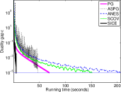
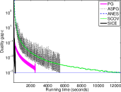
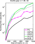
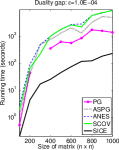
Figure 1: Left panel: duality gap attained as a function of running time (in seconds); Right panel: Time taken to reach a prescribed duality gap as a function of matrix $S$’s size.

5 Conclusions and future work

We developed, analyzed, and experimented with a powerful new algorithm for estimating the sparse inverse covariance matrices. Our method was shown to outperform all the competing state-of-the-art approaches. We attribute the speedup gains to our careful algorithmic design, which also shows that even though the spectral projected gradient method is fast and often successful, invoking it out-of-the-box can be a suboptimal approach in scenarios where the constraints were simple. In such as setup, our modified spectral approach turns out to afford significant empirical gains.

At this point several avenues of future work are open. We list them in order of difficulty: (i) Implementing our method in a multi-core or GPU setting; (ii) Extending our approach to handle more general constraints; (iii) Deriving an even more efficient algorithm that only occasionally computes gradients; (iv) Deriving a method for SICE that does not need to explicitly compute matrix inverses.

Appendix A Additional numerical results

$\epsilon$ PG ASPG ANES SCOV SICE 1E-01 0.09 0.51 0.74 0.51 0.12 1E-02 0.14 0.62 1.10 0.75 0.14 1E-03 0.26 0.94 1.73 1.16 0.16 1E-04 0.52 1.17 2.87 1.93 0.20 2E-05 0.70 1.23 3.77 2.52 0.20 1E-05 0.78 1.26 4.31 2.86 0.20	$\epsilon$ PG ASPG ANES SCOV SICE 1E-01 1.70 6.40 8.48 6.04 0.94 1E-02 7.15 13.23 18.33 13.21 1.82 1E-03 22.79 27.00 43.98 31.79 2.97 1E-04 45.38 38.91 90.84 65.76 4.44 2E-05 61.46 46.53 162.22 118.36 4.80 1E-05 68.50 46.69 206.81 151.32 4.81
$100\times 100$	$200\times 200$

$\epsilon$ PG ASPG ANES SCOV SICE 1E-01 8.46 38.97 48.05 21.75 2.28 1E-02 34.89 72.25 100.61 46.10 4.74 1E-03 127.37 142.47 214.56 98.73 7.61 1E-04 807.16 519.37 482.97 224.58 17.30 2E-05 - 1914.33 862.86 409.06 42.38 1E-05 - 2435.14 1149.04 548.34 52.29	$\epsilon$ PG ASPG ANES SCOV SICE 1E-01 16.27 84.71 109.95 109.04 5.42 1E-02 51.89 150.26 226.52 226.34 9.46 1E-03 139.73 338.29 471.29 473.33 15.59 1E-04 357.93 769.44 1020.82 1027.13 25.84 2E-05 529.69 997.44 1776.06 1793.75 28.43 1E-05 603.84 1099.55 2221.23 2106.44 30.52
$300\times 300$	$400\times 400$

$\epsilon$ PG ASPG ANES SCOV SICE 1E-01 25.28 153.41 209.90 218.42 9.55 1E-02 66.44 262.69 428.14 437.31 16.42 1E-03 307.73 731.48 901.46 911.02 29.82 1E-04 631.33 1318.33 1788.93 1828.57 45.81 2E-05 815.42 1615.56 3069.17 3117.44 61.81 1E-05 - 1719.70 3821.50 3853.45 66.20	$\epsilon$ PG ASPG ANES SCOV SICE 1E-01 28.36 275.36 391.94 379.74 16.02 1E-02 87.15 499.69 744.94 728.40 27.69 1E-03 244.11 1082.84 1446.27 1365.46 49.70 1E-04 570.52 2088.16 2777.44 2660.26 75.53 2E-05 848.27 2952.95 5049.04 4873.74 88.16 1E-05 972.13 3379.78 6383.01 6130.96 99.84
$500\times 500$	$600\times 600$

$\epsilon$ PG ASPG ANES SCOV SICE 1E-01 96.06 291.24 422.53 327.12 28.36 1E-02 271.98 520.65 796.86 618.35 54.58 1E-03 496.38 925.59 1480.13 1155.40 80.02 1E-04 863.83 1332.72 2878.07 2251.48 118.62 2E-05 1133.74 2042.25 4776.05 3736.78 134.46 1E-05 1162.10 2077.83 6106.81 4614.11 141.79	$\epsilon$ PG ASPG ANES SCOV SICE 1E-01 110.74 609.90 956.90 942.62 30.17 1E-02 320.52 880.04 1742.28 1720.76 46.54 1E-03 785.29 1742.65 3106.48 3099.92 73.06 1E-04 1742.95 3287.96 5931.33 5925.93 124.42 2E-05 2523.65 4557.51 10083.89 10018.28 175.97 1E-05 - 5470.64 12656.09 12494.52 199.07
$700\times 700$	$800\times 800$

$\epsilon$ PG ASPG ANES SCOV SICE 1E-01 88.40 635.09 1306.82 1217.88 32.21 1E-02 245.25 1153.18 2331.24 2158.39 63.42 1E-03 816.69 2862.34 4053.39 3869.56 108.35 1E-04 1604.22 5424.09 7216.28 7538.87 184.97 2E-05 2117.68 6974.25 11973.47 12710.25 211.80 1E-05 2117.68 7907.47 15083.79 15784.19 242.39	$\epsilon$ PG ASPG ANES SCOV SICE 1E-01 128.61 1005.98 1818.00 1858.70 66.08 1E-02 358.90 1712.01 3173.55 3216.55 102.48 1E-03 833.86 3529.29 5411.49 5085.51 170.25 1E-04 1405.56 5008.81 9528.91 9046.04 234.18 2E-05 - 6420.18 15964.26 15428.23 307.67 1E-05 - 7562.52 19812.06 19621.27 336.25
$900\times 900$	$1000\times 1000$

$n=100$	$n=200$

$n=300$	$n=400$

$n=500$	$n=600$

$n=700$	$n=800$

$n=900$	$n=1000$

References

- Barzilai and Borwein [1988] J. Barzilai and J. M. Borwein. Two-Point Step Size Gradient Methods. IMA Journal of Numerical Analysis, 8(1):141–148, 1988.
- Bertsekas [1999] D. P. Bertsekas. Nonlinear Programming. Athena Scientific, second edition, 1999.
- Bickel and Levina [2008] P. J. Bickel and E. Levina. Regularized estimation of large covariance matrices. Ann. Statist., 36(1):199–227, 2008.
- Bilmes [2000] J. A. Bilmes. Factored sparse inverse covariance matrices. In IEEE ICASSP, 2000.
- Birgin et al. [2000] E. G. Birgin, J. M. Martínez, and M. Raydan. Nonmonotone Spectral Projected Gradient Methods on Convex Sets. SIAM Journal on Optimization, 10(4):1196–1211, 2000.
- Byrd et al. [1995] R. Byrd, P. Lu, J. Nocedal, and C. Zhu. A Limited Memory Algorithm for Bound Constrained Optimization. SIAM J. Sci. Comp., 16(5):1190–1208, 1995.
- Dai and Fletcher [2005] Y. H. Dai and R. Fletcher. Projected Barzilai-Borwein Methods for Large-scale Box-constrained Quadratic Programming. Numerische Mathematik, 100(1):21–47, 2005.
- d’Aspremont et al. [2008] A. d’Aspremont, O. Banerjee, and L. E. Ghaoui. First-order methods for sparse covariance selection. SIAM J. Matrix Anal. Appl., 30(1):56–66, 2008.
- Dempster [1972] A. P. Dempster. Covariance selection. Biometrics, 28(1):157–175, 1972.
- Dobra et al. [2004] A. Dobra, C. Hans, B. Jones, J. R. Nevins, and M. West. Sparse graphical models for exploring gene expression data. Journal of Multivariate Analysis, 90:196–212, 2004.
- Duchi et al. [2008] J. Duchi, S. Gould, and D. Koller. Projected subgradient methods for learning sparse Gaussians. In Proc. Uncertainty in Artificial Intelligence, 2008.
- Friedlander et al. [1995] A. Friedlander, J. M. Martínez, and M. Raydan. A New Method for Large-scale Box Constrained Convex Quadratic Minimization Problems. Optimization Methods and Software, 5:55–74, 1995.
- Friedman et al. [2008] J. Friedman, T. Hastie, and R. Tibshirani. Sparse inverse covariance estimation with the graphical lasso. Biostatistics, 9:432–441, 2008.
- Grippo and Sciandrone [2002] L. Grippo and M. Sciandrone. Nonmonotone Globalization Techniques for the Barzilai-Borwein Gradient Method. Computational Optimization and Applications, 23:143–169, 2002.
- Huang et al. [2006] J. Z. Huang, N. Liu, M. Pourahmadi, and L. Liu. Covariance matrix selection and estimation via penalised normal likelihood. Biometrika, 93(1):85–98, 2006.
- Kim et al. [2007] S. Kim, K. Koh, M. Lustig, S. Boyd, and D. Gorinevsky. An Interior-Point Method for Large-Scale -Regularized Least Squares. IEEE J. Selected Topics in Signal Processing, 1:606–617, Dec. 2007.
- Lauritzen [1996] S. L. Lauritzen. Graphical Models. OUP, 1996.
- Lu [2009] Z. Lu. Smooth optimization approach for sparse covariance selection. SIAM J. Optim. (SIOPT), 19(4):1807–1827, 2009.
- Lu [2010] Z. Lu. Adaptive first-order methods for general sparse inverse covariance selection. SIAM J. Matrix Analysis and Applications (SIMAX), 31(4):2000–2016, 2010.
- Malioutov et al. [2006] D. M. Malioutov, J. K. Johnson, and A. S. Willsky. Walk-Sums and Belief Propagation in Gaussian Graphical Models. JMLR, 7:2031–2064, 2006.
- Meinshausen and Bühlmann [2006] N. Meinshausen and P. Bühlmann. High-dimensional graphs and variable selection with the lasso. The Annals of Statistics, 34(3):1436–1462, 2006.
- Mood et al. [1974] A. M. Mood, F. A. Graybill, and D. C. Boes. Introduction to the theory of statistics. McGraw-Hill, 1974.
- Nesterov [2005] Y. Nesterov. Smooth minimization of non-smooth functions. Math. Program., Ser. A, 103:127–152, 2005.
- Nesterov and Nemirovski [1994] Y. E. Nesterov and A. S. Nemirovski. Interior-Point Polynomial Algorithms in Convex Programming: Theory and Applications. SIAM, 1994.
- Raydan [1993] M. Raydan. On the Barzilai and Borwein Choice of the Steplength for the Gradient Method. IMA Journal on Numerical Analysis, 13:321–326, 1993.
- Raydan [1997] M. Raydan. The Barzilai and Borwein gradient method for the large scale unconstrained minimization problem. SIAM J. Opt., 7(1):26–33, 1997.
- Rosen [1960] J. B. Rosen. The Gradient Projection Method for Nonlinear Programming. Part I. Linear Constraints. Journal of the Society for Industrial and Applied Mathematics, 8(1):181–217, 1960.
- Rothman et al. [2008] A. J. Rothman, P. J. Bickel, E. Levina, and J. Zhu. Sparse permutation invariant covariance estimation. Electron. J. Statist., 2:494–515, 2008.
- Rue and Held [2005] H. Rue and L. Held. Gaussian Markov Random Fields. Chapman and Hall/CRC, 2005.
- Schmidt et al. [2009] M. Schmidt, E. van den Berg, M. Friedlander, and K. Murphy. Optimizing Costly Functions with Simple Constraints: A Limited-Memory Projected Quasi-Newton Algorithm. In AISTATS, 2009.
- Wainwright and Jordan [2008] M. J. Wainwright and M. I. Jordan. Graphical Models, Exponential Families, and Variational Inference. Found. Trends Mach. Learn., 1(1-2):1–305, 2008.