Warm H₂O and OH disk emission in V1331 Cyg

Abstract

We present high resolution ($R=24,000$) $L$-band spectra of the young intermediate mass star V1331 Cyg obtained with NIRSPEC on the Keck II telescope. The spectra show strong, rich emission from water and OH that likely arises from the warm surface region of the circumstellar disk. We explore the use of the new BT2 (Barber et al., 2006) water line list in fitting the spectra, and we find that it does a much better job than the well-known HITRAN (Rothman et al., 1998) water line list in the observed wavelength range and for the warm temperatures probed by our data. By comparing the observed spectra with synthetic disk emission models, we find that the water and OH emission lines have similar widths (FWHM $\simeq 18\,{\rm km}\,{\rm s}^{-1}$). If the line widths are set by disk rotation, the OH and water emission lines probe a similar range of disk radii in this source. The water and OH emission are consistent with thermal emission for both components at a temperature $\sim 1500$ K. The column densities of the emitting water and OH are large, $\sim 10^{21}\,\rm\,cm^{-2}$ and $\sim 10^{20}\,\rm\,cm^{-2}$, respectively. Such a high column density of water is more than adequate to shield the disk midplane from external UV irradiation in the event of complete dust settling out of the disk atmosphere, enabling chemical synthesis to continue in the midplane despite a harsh external UV environment. The large OH-to-water ratio is similar to expectations for UV irradiated disks (e.g., Bethell & Bergin, 2009), although the large OH column density is less easily accounted for.

1 Introduction

Near-infrared ro-vibrational emission lines of water and OH are probes of the physical and chemical conditions in the warm inner regions of gaseous disks surrounding young stars (e.g., Carr et al., 2004; Najita et al., 2007). Water emission has been detected previously in the $K$-band from high accretion rate systems ($>10^{-7}M_{\odot}\,{\rm yr}^{-1}$), ranging from low mass objects such as SVS 13 (Carr et al., 2004) and DG Tau (Najita et al., 2000), to higher mass objects such as V1331 Cyg (Najita et al., 2009) and [BKH2005] 08576nr292 (Thi & Bik, 2005). The water emission in these systems is accompanied by $2.3~{}\mu$m CO overtone emission that also arises from the inner disk. In the lower mass objects in which water emission is detected, the emission arises from within $\sim 0.5$ AU. In all systems the emission column densities are large ($\sim$10¹⁸–10${}^{21}\rm\,cm^{-2}$) and the temperature of the emitting gas is high ($\sim$1500 K).

These observations complement studies of water emission made at mid-infrared wavelengths with the Spitzer Space Telescope and ground-based facilities (Carr & Najita, 2011, 2008; Pontoppidan et al., 2010a; Salyk et al., 2011, 2008; Pontoppidan et al., 2010b; Knez et al., 2007) and longer wavelength studies with the Herschel Space Telescope (e.g., Sturm et al., 2010), which measure cooler water, probably arising at larger disk radii on average. The mid-infrared water emission arises from systems spanning a wide range of accretion rates, including typical T Tauri stars such as AA Tau (Carr & Najita, 2008, $\lesssim 10^{-8}\,M_{\odot}\,{\rm yr}^{-1}$) and high accretion rate T Tauri stars such as DR Tau and AS 205A (Salyk et al., 2008, $\gtrsim 10^{-7}\,M_{\odot}\,{\rm yr}^{-1}$). Perhaps because the mid-infrared water emission can arise under a wide range of conditions, it appears commonly in Spitzer spectra of T Tauri stars (Carr & Najita, 2011; Salyk et al., 2011; Pontoppidan et al., 2010a).

Ro-vibrational OH emission is also believed to arise from the inner regions of gaseous disks. OH emission in the $L$-band has been previously reported from V1331 Cyg and SVS 13 (Najita et al., 2007), and from DR Tau and AS 205A (Salyk et al., 2008). All of these sources also show H₂O emission in their $L$-band spectra. OH emission has also been detected from Herbig stars; the $L$-band spectra of these sources is notably lacking in water emission (Mandell et al., 2008; Fedele et al., 2011). The $L$-band OH emission in the Mandell sources has temperatures of 650–1000 K, and column densities of $\sim$ 10¹⁴–10${}^{17}\rm\,cm^{-2}$.

Here we present high-resolution $L$-band spectra of V1331 Cyg (LkHa 120), a young star in the L988 dark cloud complex. Previous studies of this source have suggested a spectral type (A8–G5, Kuhi, 1964; Chavarría, 1981; Hamann & Persson, 1992) that is intermediate between those of Herbig Ae stars and typical T Tauri stars. There are various estimates of the distance to the source (for a summary see Herbig & Dahm, 2006), with extinction studies of the region toward the L988 dark clouds suggesting a distance of $\sim 550$ pc. The accretion rate of V1331 Cyg is high. The Br$\gamma$ line flux measured by Eisner et al. (2007) corresponds to an accretion luminosity of $8.5L_{\odot}$ at a distance of 550 pc, putting the accretion rate at $>3\times 10^{-7}M_{\odot}\,{\rm yr}^{-1}$.

As noted above, OH emission from V1331 Cyg has been previously reported, based on a small portion of the $L$-band spectrum (Najita et al., 2007). The data presented here cover a much larger wavelength range, allowing us to constrain the properties of the molecular emission in this spectral region. This study complements our earlier study of CO overtone and water emission in the $K$-band spectrum of V1331 Cyg (see also Najita et al., 2009; Carr, 1989).

In our previous studies of water emission, we used a water line list that was constructed from the Partridge & Schwenke (1997) and HITRAN line lists and refined empirically in the small portion of the $K$-band that we studied (Carr et al., 2004). Here we explore the use of the new BT2 water line list (Barber et al., 2006) in modeling a much larger wavelength region.

2 Observations

2.1 Spectroscopy

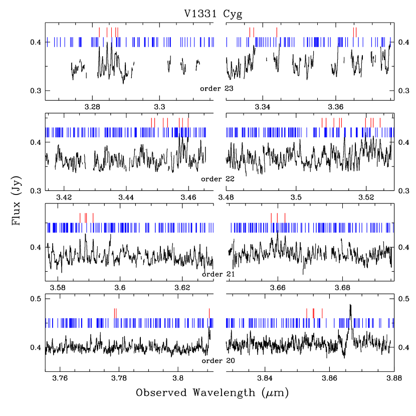
Figure 1: High signal-to-noise (SNR $>$150), high resolution ($R\equiv\lambda/\Delta\lambda=24,000$) spectra of V1331 Cyg spanning 4 $L$-band orders observed with NIRSPEC at two grating settings. Emission lines of water (lower ticks, blue) and OH (upper ticks, red) are evident throughout these $L$-band spectra. Lines within 10% of the strongest line in the BT2 list for each order were selected here. Wavelength regions where the telluric transmission was poor (i.e., $\leq$ 80%) have been excised from the plots.

High resolution $L$-band spectra of V1331 Cyg were taken on 11 July 2001 with NIRSPEC (McLean et al., 1998), the multi-order cryogenic echelle facility spectrograph on Keck II. The data were obtained by one of us (JRG) through time granted to our NASA/Keck proposal. The spectra cover most of the $L$-band at a resolution of $R\equiv\lambda/\delta\lambda$ = 24,000 ($12.5\,{\rm km}\,{\rm s}^{-1}$) using the 0.432$\arcsec$ (3-pixel wide) slit. The echelle orders overfill the detector in the dispersion direction, and therefore wavelength coverage of most of the $L$-band was achieved in two grating setups. In the first setup (hereafter L1), the echelle and cross disperser angles were oriented at $62.2^{\circ}$ and $33.15^{\circ}$, respectively. In the second setup (hereafter L2), the echelle and cross disperser angles were oriented at $64.3^{\circ}$ and $33.29^{\circ}$, respectively. Both grating setups imaged separate portions of orders 20–25 onto the 1024 $\times$ 1024 InSb detector array through the KL filter. Poor telluric transmission in orders 24 and 25 (at $3.2~{}\mu$m and $3.1~{}\mu$m) prevented our using any data at these grating settings, thus our analysis used the spectra we obtained in orders 23–20 (3.27–3.88$~{}\mu$m, Fig. 1).

To obtain both object and sky spectra, we nodded the telescope along the $24\arcsec$ long slit in three positions in an ABC nod pattern, with one position centered on the slit and the two others offset by $-8\arcsec$ and $+8\arcsec$ relative to the slit center. Single exposures of V1331 Cyg were 30 seconds $\times$ 4 co-adds at each nod position, resulting in 12 minutes of total integration time in $\sim 0\farcs 5$ seeing (FWHM $L$-band) within an airmass range of 1.35–1.45. During the observations, the instrument image rotator was kept in stationary mode, keeping the slit physically stationary and thus allowing it to slowly rotate on the sky as the alt-az mounted Keck II telescope tracked.

To remove telluric absorption features, spectra of an early type star (HR 7610, A1 IV) were taken immediately following the V1331 Cyg observations using the same two grating configurations successively over a similar airmass range (1.3–1.4). Spectra of the NIRSPEC internal continuum lamp were used for flat-fielding. We used telluric absorption lines identified in the spectra of our target and calibration stars for wavelength calibration.

2.2 Data Reduction

Initially, bad pixels present in the raw object, telluric, and calibration frames were identified and removed by interpolation using the fixpix algorithm within the REDSPEC reduction package (a custom echelle reduction package developed by Prato, Kim, and McLean).

Standard IRAF packages (Massey et al., 1992, 1997) were used to reduce the data. Pairs of exposures taken at different nod positions closest in time were differenced then divided by the normalized internal continuum lamp frame for adequate sky subtraction and flatfielding. Each echelle order on the array was then rectified using selected bright sky emission lines (typically 9–12 lines) present in the object frame, summed over all nod positions. Exposures taken at the same nod position were summed after accounting for any slight spatial offsets (to within a single pixel).

Object and telluric calibration spectra at each nod position in each echelle order were then extracted from a spatial profile that was $\gtrsim$ 10% of the profile peak (i.e., 3–4 pixels), using a background aperture off the peak (e.g., $\pm$ 8–28 pixels) for residual background correction. Each extracted object and telluric spectrum was wavelength calibrated using selected telluric absorption lines identified from the HITRAN database (Rothman et al., 1998).

Telluric features in each of the three nod positions of V1331 Cyg were removed by dividing by the spectrum of the telluric standard taken at the same nod position along the slit. An optimal telluric cancellation in V1331 Cyg was achieved using the IRAF package telluric, which allowed the strengths of the telluric lines to be scaled to account for a slight difference in the airmass of the hot standard star before normalization and division with the target spectra.

We put our V1331 Cyg spectra on a flux scale using photometry from the literature. We constructed an SED for V1331 Cyg, using the near-IR and optical photometry of 2MASS and Chavarría (1981), respectively. The 2MASS $K$-band photometric point is in good agreement with the flux calibrated $K$-band spectra from Najita et al. (2009). We fit the near-IR photometry with a low order function to interpolate the expected flux in different $L$-band orders. We then rescaled our NIRSPEC observations so that the flux average in each observed order matched the interpolated value from the SED ($\sim$ 0.35–0.41 Jy across 3.291–3.854 $\mu$m).

3 Analysis

The resulting $L$-band spectra of V1331 Cyg reveal emission features that are strong, numerous, and relatively narrow (Fig. 1). The narrow line widths are an advantage in deconstructing such a rich emission spectrum. The coincidence between the observed emission features and the wavelengths of lines of OH (red ticks) and water (blue ticks) suggest that the observed spectra are dominated by emission from water and OH. As we show below, the spectra are consistent with OH and water emission from the atmosphere of the inner disk of V1331 Cyg (Figs. 2a–h). From the line widths and strengths, we characterize the physical conditions in the disk where the water and OH emission arises.

3.1 Disk Emission Model

The radial velocity of the observed features has a topocentric value of –27.6 ${\rm km}\,{\rm s}^{-1}$, in agreement with the radial velocity of the C¹⁸O (2-1) emission from the envelope which provides an estimate of the radial velocity of the system (v${}_{\rm LSR}=-1.3\,{\rm km}\,{\rm s}^{-1}$, McMuldroch, 1993). The lack of a velocity offset with respect to the systemic velocity is consistent with an origin for the emission in a rotating circumstellar disk.

We therefore modeled the observed spectra of V1331 Cyg by combining contributions from the stellar continuum, a disk veiling continuum, and emission lines of H₂O and OH from a disk atmosphere. The disk line emission model, which follows the approach described in Carr et al. (2004), assumed the geometry of a plane parallel slab of gas in a Keplerian disk that is in vertical hydrostatic equilibrium. The parameters describing the slab are the gas temperature ($T$), column density ($N$), and intrinsic line broadening, the inner and outer radii of the emission ($R_{\rm in}$, $R_{\rm out}$), and the line-of-sight disk rotational velocity at the inner radius of the emission ($v\sin i$).

The molecular emission spectrum can be used to constrain these parameters in the following schematic way. The relative strengths of the emission features constrain the temperature ($T$) and column density ($N$) of the emission. The large number of transitions in the spectrum and the wide range in their intrinsic strengths ($gf$-values) and energy levels are assets in this regard. The flux level of the emission spectrum constrains the projected emitting area for the emission, which is a function of $R_{\rm in}$ and $R_{\rm out}$, the inclination, and the assumed distance to the system.

The V1331 Cyg emission lines are resolved, narrow, and centrally peaked. Because the emission lines are resolved, we have a further constraint on the emitting radii. The maximum velocity of the emission profile (i.e., the velocity extent of the profile) constrains the projected velocity at the inner radius of the emission ($v\sin i$). The values of $R_{\rm in}$ and $v\sin i$, along with an assumed stellar mass, specify the inclination of the system.

The shape of the emission profile constrains the outer radius of the emission ($R_{\rm out}$), e.g., a small ratio of $R_{\rm out}/R_{\rm in}$ produces a double-peaked profile, whereas a large ratio produces a centrally-peaked profile. In modeling the spectrum we find that the centrally peaked profile cannot be fit with $R_{\rm out}/R_{\rm in}<2.0$; therefore the emission must arise over a range of radii and not from a narrow annulus.

The temperature and column density may also vary with radius and can affect the detailed line profile shape. Because the line profiles are only marginally resolved in our data, our ability to diagnose these properties is limited. We therefore assume a constant temperature and column density for the emitting region in the modeling carried out here.

Thus our strategy was to search for a combination of temperature and column density that fit the relative line strengths and then choose an emitting area (i.e., an outer radius) that matched the overall flux of the lines for the assumed distance. The combination of an observed $v\sin i$, an emitting area inferred from the emission flux, and a constraint on $R_{\rm out}/R_{\rm in}$ from the line profile then allowed us to constrain the model parameters $R_{\rm out}$, $R_{\rm in}$, and the inclination $i$. We required that the model provide a decent fit to all four of the orders observed with the L1 and L2 grating settings.

The additional parameters in the modeling are the stellar mass and the distance and extinction to the source. For consistency with our earlier study of the $K$-band water and CO emission from this source (Najita et al., 2009), we adopted a distance of 550 pc (Shevchenko et al., 1991; Alves et al., 1998), a stellar mass of $1.8M_{\odot}$, and no $K$-band extinction along the line of sight. Also consistent with our earlier study, we assumed a stellar radius and temperature of $2.2R_{\odot}$ and $7200$ K, respectively, and we estimated the underlying stellar $L$-band continuum assuming a blackbody function. As noted in Najita et al. (2009), the stellar properties are not well known.

We constructed separate syntheses for the OH and water emission, and then combined the models additively. This is an acceptable approach because there is little overlap between the lines from the water and OH line lists to within several ${\rm km}\,{\rm s}^{-1}$, despite the high density of water lines in the BT2 list. To determine the strength of the disk veiling continuum, we started with the stellar contribution to the $L$-band continuum and added the synthesized water emission spectrum. Disk continuum emission was then added to bring the model emission up to the observed level of the emission in each order. The required amount of disk continuum emission increased monotonically from $\sim 0.26$ Jy to $\sim 0.37$ Jy across $L$-band orders 23 to 20, consistent with the SED shape of V1331 Cyg ($\S$2.2). Since most of the $L$-band continuum is dominated by the excess disk emission (i.e., veiling of approximately 10 in the $L$-band), no stellar spectral features would be detectable in our data. As the last step, a synthetic OH emission spectrum was added to produce the final model spectrum (Figs. 2a–h).

3.2 Molecular Linelists

A successful model requires good line lists. Our OH line list comes from the HITRAN database (Rothman et al., 1998), an empirically determined list based on absorption in the Earth’s atmosphere. Many of the OH emission lines in our $L$-band spectra are prominent and mostly isolated from one another, allowing us to identify the transitions present in our data.

For water, we use a new theoretical line list, BT2 (Barber et al., 2006), which includes over 500 million transitions. We trimmed the line list to a parameter range that is relevant for the present application, by sorting lines based on their relative strengths at 1500K, the approximate temperature we found in fitting the $K$-band water emission of V1331 Cyg. Here the relative strength is the product of the absorption cross section and the fractional population in the lower energy level of the transition. We excluded lines that had relative strengths $<0.001\%$ of the strongest line in each order. The resulting line list included $\sim$4600 to $\sim$6700 lines in each of our $L$-band orders.

3.3 Water and OH emission in the $L$-band

We find that we can fit the water emission line profile and reproduce much of the water emission structure we observe with a temperature of $\sim 1500$ K, a line-of-sight H₂O column density of $\sim 2\times 10^{21}\rm\,cm^{-2}$, an emitting area extending from $R_{\rm in}=5.5R_{\odot}$ to $R_{\rm out}=3.5R_{\rm in}$ (i.e., 0.03–0.09 AU), and $v\sin i=14\,{\rm km}\,{\rm s}^{-1}$ at $R_{\rm in}$. The resulting emission profile is convolved with the 3-pixel NIRSPEC slit resolution of $12.5\,{\rm km}\,{\rm s}^{-1}$. We refer to the model with these parameters as our “reference model” for the water emission (Figs. 2a–h). As the fits demonstrate, the line emission is dominated by water in all observed $L$-band orders. The water lines detected in the various $L$-band orders span a broad range from optically thin to thick (e.g., $\tau_{H_{2}O}\sim 10^{-3}$ to $10^{2}$ for the reference model).

These values for the water temperature and column density are similar to the fit we found previously to the $K$-band water emission observed in V1331 Cyg (Najita et al., 2009). The emitting area we derive for the $L$-band water emission is somewhat smaller than ($\sim$ 50% of) the size of the $K$-band emitting area found in the earlier study. This difference does not mean that the results are in conflict, because the $K$- and $L$-band observations were taken at different epochs and the line emission strength may vary. But it is also unclear whether variability is indicated because the present data were flux calibrated using data from the literature rather than contemporaneous observations ($\S$2).

An inner radius of 5.5$R_{\odot}$ is 2.5 times larger than the stellar radius of 2.2$R_{\odot}$ ($\S$3.1). For a stellar mass of $1.8M_{\odot}$ ($\S$3.1), the adopted values of $v\sin i$ and $R_{\rm in}$ correspond to an inclination of 3 degrees. The inclination and the range of emission radii are consistent with the values we found in modeling the $K$-band water emission from this source (Najita et al., 2009).

The inferred values for $R_{\rm in},$ $R_{\rm out}$, and inclination depend on the assumed distance to the source and the stellar mass, neither of which are well known. The distance has been variously estimated in the range 500–800 pc (Najita et al. 2009), allowing for larger values than we assumed. A larger distance would require a larger disk emitting area to produce the same flux. For those larger disk emitting radii, a larger inclination would be needed to produce the same $v\sin i$ at a fixed stellar mass. However, a larger distance would also affect the estimate of the stellar mass based on the SED, with further consequences for the $R_{\rm in}$, $R_{\rm out}$, and inclination. Because of these uncertainties, the values of $R_{\rm in}$, $R_{\rm out}$, and inclination are not well constrained by our modeling. Nevertheless, the modeling shows that the notional values of stellar mass and distance from the literature do allow for a simple disk model for the molecular emission.

To estimate the range of column density (or temperature) that would produce a reasonable fit to the water emission, we held temperature (or column density) fixed at the value of the reference model and allowed column density (or temperature) to vary with emitting area as a free parameter. The emitting area was determined by fitting the spectrum in L1 order 21, and the value was kept the same for all other orders. L1 order 21 was chosen since it contained a mix of optically thick and thin lines and is a spectral region with relatively good telluric transmission. We determined the value of the emitting area by minimizing the sum of the absolute values of the pixel differences between the observed spectrum and the model in L1 order 21 (Branham, 1982). Regions with poor telluric transmission (i.e., $<$ 80%) were excluded in this estimate.

Figure 3a shows the resulting fits to L1 order 21 at a fixed temperature (T=1500 K) for the reference model (middle spectrum) and for column densities 10 times lower (upper spectrum) and 10 times higher (lower spectrum). The low column density model is more optically thin and has larger peak-to-trough variation, while the high column density model has much less contrast. The peak-to-trough variation in the reference model more closely resembles that of the observed spectrum. Figure 3b shows the model results for a neighboring order (L1 order 22) obtained with the same emitting area used in L1 order 21. The low and high column density models fit much worse than in L1 order 21 because the emitting area was not optimized for this order. These model fits are clearly worse than the reference model in fitting the observed spectrum.

Figure 4a shows fits to L1 order 21 for the reference model temperature (middle spectrum) and for lower (upper spectrum) and higher (lower spectrum) temperatures. The lower temperature model has too large a peak-to-trough variation, while the higher temperature model has too little, compared with the reference model case (1500 K). This same trend is evident in another order (L1 order 22, Fig. 4b). In both figures, the high and low temperature models are clearly worse than the reference model case. Therefore, for the water emission it appears that we can rule out column densities $\leq 2\times 10^{20}$ and $\geq 2\times 10^{22}\rm\,cm^{-2}$ and temperatures $\leq 1200$ K and $\geq 2000$ K.

We adopted a similar approach in fitting the OH emission. We found that the OH emission lines in our $L$-band data can be fit with a temperature of $\sim 1500$ K and a line-of-sight OH column density of $\sim 1\times 10^{20}\rm\,cm^{-2}$, and a larger emitting area (2.1 times larger) than the water emission, with radii extending from $R_{\rm in}=5.5R_{\odot}$ to $R_{\rm out}=5R_{\rm in}$, and $v\sin i=14\,{\rm km}\,{\rm s}^{-1}$ at $R_{\rm in}$. We refer to the model with these parameters as our “reference model” for the OH emission (Fig. 2a–h). The difference between the emitting areas of water and OH in the reference model is not significant. If we assume the OH emission comes from the same range of radii as the water emission ($R_{\rm in}=5.5R_{\odot}$ to $R_{\rm out}=3.5R_{\rm in}$), then we find a similar fit to the OH emission at the same column density as above, but at a slightly higher temperature ($1850$ K). The OH lines in our spectra range from optically thin to thick, depending on the transition and model parameters (e.g., $\tau_{OH}\sim 0.1$ to $30$ for the reference model, Table 1). The OH transitions also span a range in excitation, including 1–0 lines with J = 11, 12, 14-18 and 2–1 lines with J = 8-18 (red ticks, Fig. 2a–h, see Table 1). Since the OH lines in our data span a range of optical depths and excitation levels, we can constrain the column density and temperature of the model fits.

By requiring a consistent fit to all orders we can exclude column densities $\leq 5\times 10^{19}$ and $\geq 10^{21}\rm\,cm^{-2}$ and temperatures $\leq 1200$ K and $\geq 2300$ K. Figure 5a compares observed spectral regions where OH is present (black histogram) with model fits that include H₂O and OH and adopt higher and lower OH column densities than the reference OH model at a fixed temperature (T=1500 K). The top panel compares the reference model (N=$1\times 10^{20}\rm\,cm^{-2}$, solid blue line) with a low column density fit (N=$5\times 10^{19}\rm\,cm^{-2}$; dotted red line). The low column density model overpredicts the flux of the lines at shorter wavelengths (3.282-3.287 $\mu$m). The bottom panel compares the reference model (N=$1\times 10^{20}\rm\,cm^{-2}$, solid blue line) with a high column density fit (N=$1\times 10^{21}\rm\,cm^{-2}$, dotted red line). The high column density model underpredicts the flux of the lines at shorter wavelengths (3.282-3.287 $\mu$m) and somewhat overpredicts the flux of the lines at longer wavelengths (3.776-3.780 $\mu$m). The reference model fits all the OH lines adequately well across a range of optical depths.

Similarly, Figure 5b compares selected OH lines (black histogram) with fits at higher and lower temperatures than the reference OH model at a fixed column density (N=$1\times 10^{20}\rm\,cm^{-2}$). The top panel compares the reference model (T=1500 K, solid blue line) with a low temperature fit (T=1200 K; dotted red line). The low temperature model overpredicts the flux of the low-J lines at shorter wavelengths (3.282-3.287 $\mu$m). The bottom panel compares the reference model (T=1500 K, solid blue line) with a high temperature fit (T=2300 K, dotted red line). The high temperature model overpredicts the flux of the high-J lines at longer wavelengths (3.776-3.780 $\mu$m). The low temperature model puts too much energy into the low-J lines (shorter wavelengths, top panel), and the high temperature model puts too much energy into the high-J lines (longer wavelengths, bottom panel). The reference model fits all the OH lines adequately well across a range of excitation levels.

The good agreement between the observed spectrum and the OH+H₂O model spectrum (Fig. 2) shows that it is possible to account for much of the spectral structure with our reference model of molecular emission from a rotating disk. The temperature of the water and OH emission fit by the reference models is the same ($\sim 1500$ K for both), while the OH column is $\sim 10$ times less than the water column. The range of emitting radii for both models overlaps, with the emission from both species arising from within 0.2 AU of the star. Some discrepancies between the observed and model spectra are noticeable and may be attributed to errors in the transition frequency and/or oscillator strength of some lines in the BT2 water line list (e.g., features at 3.485 $\mu$m, 3.492 $\mu$m, 3.499 $\mu$m, 3.505 $\mu$m, 3.514 $\mu$m; vertical arrows in Fig. 2c).

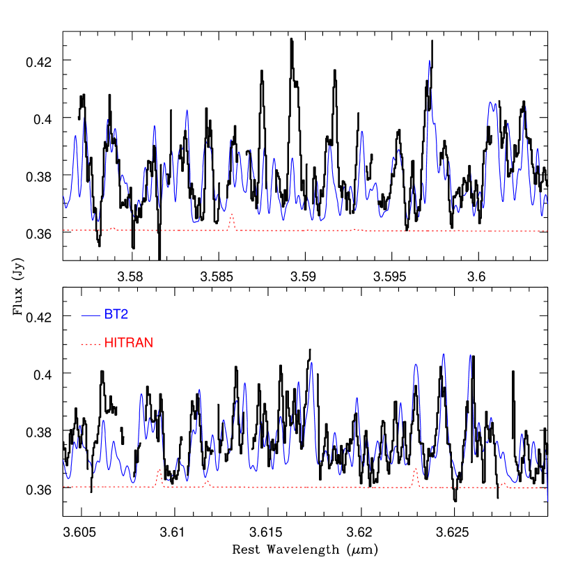
Figure 6: A comparison of synthetic spectra at the same temperature ($T=1500\,$K), H₂O column density ($2\times 10^{21}\rm\,cm^{-2}$), and emitting area (5.5 $<R_{\rm H_{2}O}/R_{\odot}<19$) as was found for the reference model to V1331 Cyg, but generated using different water line lists. The model using the BT2 water list (solid blue line) fits most of the observed structure in V1331 Cyg (black histogram), while the model from the HITRAN water line list (dotted red line) does a poor job fitting the data (thick black histogram), with very few emission features present arising from a depressed continuum level.

The advantage of using the BT2 list, compared to the more familiar HITRAN list, when studying warm water emission is apparent if we compare synthetic spectra produced with the two line lists at a temperature of 1500 K (Fig. 6). While the fit parameters are identical in both cases, the BT2 list clearly matches most of the observed structure in the data, while the HITRAN list misses most of it. This is because of the absence of high temperature lines in HITRAN, which are present in the BT2 list. For water emission at lower temperatures ($\sim 1000$ K) and in wavelength regions dominated by low excitation lines, the HITRAN list can do about as well as BT2, as in the case of the $2.9~{}\mu$m water emission observed in AS 205A and DR Tau (Salyk et al., 2008).

The line widths of individual OH and H₂O lines are difficult to measure directly from our data owing to the crowding of numerous H₂O lines throughout the $L$-band. In the absence of microturbulent broadening, the intrinsic line widths of the molecular emission we detect in our observations is determined by pure thermal broadening, which is $\sim$1 ${\rm km}\,{\rm s}^{-1}$ in our case for both H₂O and OH at 1500K, and 0.8 ${\rm km}\,{\rm s}^{-1}$ for CO at 1800 K. The modeling results show that the $L$-band ro-vibrational water and OH emission in this source have similar emission line profiles (FWHM $\sim$ 17–20 ${\rm km}\,{\rm s}^{-1}$), indicating that emission lines in both species arise from a similar range of disk radii. Thus it seems plausible that the two species probe similar gas temperatures. If this is the case, it implies that the ratio of OH and water column densities is $\sim 0.1$.

3.4 Water and CO emission in the $K$-band

Water and CO emission from V1331 Cyg has been previously reported in the $K$-band (Najita et al., 2009), based on an observation made in 1999, two years earlier than the observation date of the $L$-band data reported here. To determine how the OH and water emission properties in the $L$-band compare with those of CO and water reported in the $K$-band study, we re-analyzed the $K$-band data using the same simple slab model described in $\S$3.1. Our analysis here differs in several ways from the previous analysis (Najita et al., 2009) in that we report a single fixed temperature and column density for each species rather than using radial gradients, and chemical equilibrium is not assumed for either species. Our analysis also uses the new BT2 line list, compared with a previous water line list that was empirically calibrated but for a limited region near the 2–0 CO bandhead (i.e., Carr et al., 2004).

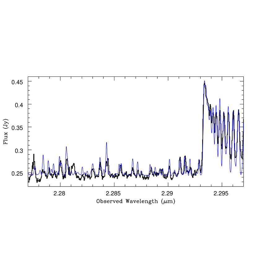
Figure 7: A fit to the $K$-band spectrum of V1331 Cyg observed in an earlier epoch (thick histogram, Najita et al. 2009), showing strong water emission blueward of the overtone CO emission bandhead. The model fit, a combination of water and CO emission (thin blue line), does a good job fitting the observed structure, highlighting the utility of the BT2 list in fitting warm $K$-band water emission. The fit parameters for the water emission in the $K$-band are the same as for the water in the $L$-band (i.e., Fig. 2), except for having an emitting area that is 1.6 times larger, which could be ascribed to time variable emission and/or uncertainties in the flux calibration between the two observational epochs. The CO model has a temperature of 1800 K, a column density of $6\times 10^{21}\rm\,cm^{-2}$, and an emitting area extending from $R_{\rm in}=2.3R_{\odot}$ to $R_{\rm out}=8R_{\rm in}$ (see Table 2).

We find a good fit to the water features in the $K$-band using the same parameters found for the $L$-band (i.e., $T_{\rm H_{2}O}=1500~{}$K and $N_{\rm H_{2}O}=2\times 10^{21}\rm\,cm^{-2}$), but with an emitting area that is 2 times larger (i.e., $R=5.5-26~{}R_{\odot}$). It is possible that the different values we find for the emitting area of water in V1331 Cyg over different observational epochs result from real time variability in the emission, but some fraction of the difference could also be accounted for by uncertainties in the flux calibration in either epoch. Guided by the previous fit values for CO, we found we could fit the CO emission reasonably well with a temperature of $T_{\rm CO}=1800$ K and a line-of-sight column density $N_{\rm CO}=6\times 10^{21}\rm\,cm^{-2}$, that emits over disk radii 2.3–18 $R_{\odot}$, with $v\sin~{}i=23\,{\rm km}\,{\rm s}^{-1}$ at $R_{\rm in}$ and turbulent broadening of $v_{\rm turb}=4\,{\rm km}\,{\rm s}^{-1}$ (Fig. 7). The BT2 list does a good job reproducing most of the emission structure observed blueward of the CO bandhead (Fig. 7), and discrepancies in the fit to the data may illustrate the need for empirical calibration of its line strengths and transition energies in the $K$-band as well. The inner radius for the emission may appear uncomfortably close to the stellar radius ($2.2R_{\odot}$; §3.1). We note that the inferred disk emitting radii are not well constrained by our modeling and larger emitting radii are possible, in principle, with a larger source distance (§3.3). A more complete modeling effort that explores the uncertainty in the source distance is needed to explore this possibility.

From our analysis of the $K$-band data, we find a CO-to-water column density ratio of $\sim$ 3–10, consistent with the results of Najita et al. (2009). The larger value would apply if the water emission has the same value of $v_{\rm turb}=4\,{\rm km}\,{\rm s}^{-1}$ as the CO emission. The smaller value would apply if the water emission has no turbulent broadening, as in the $L$-band modeling. The CO and water emission may experience different amounts of turbulent broadening if they are produced at different heights or radii in the disk atmosphere. We compare in Table 2 the results of the $K$-band modeling with the properties of the reference model for the $L$-band modeling. As shown in Table 2, the properties of the water emission observed in the $K$- and $L$-bands are quite similar.

4 Discussion

4.1 Comparison to other sources with disk emission

To date, gaseous water and OH emission have been reported in the near-IR spectra of only a handful of young stars (Carr et al., 2004; Najita et al., 2000; Thi & Bik, 2005; Salyk et al., 2008; Mandell et al., 2008; Najita et al., 2009; Fedele et al., 2011). As noted in $\S$3.3, the water emission temperature ($\sim 1500$ K) and column density ($\sim 10^{21}\,\rm\,cm^{-2}$) that we find for V1331 Cyg are similar to the water emission properties reported for V1331 Cyg based on its $K$-band spectrum (Najita et al., 2009). These properties are also similar to those found for the near-IR water emission detected from SVS 13 (Carr et al., 2004), for which the radii of emission are comparably small ($\lesssim 0.3$ AU). The water emission detected from the disk surrounding the high mass star 08576nr292 ($6M_{\odot}$) was also found to have a similar temperature but a significantly lower column density ($\sim 10^{18}\,\rm\,cm^{-2}$) emitting over a larger area from an inner radius of 2 AU to an outer radius of 4 AU (Thi & Bik, 2005).

In comparison to the T Tauri stars, AS 205 and DR Tau (Salyk et al., 2008), which also show water emission in the $L$-band, the emission spectrum of the more extreme T Tauri star V1331 Cyg, reported here, is much richer (i.e., has a higher density of emission lines), probably as a consequence of its higher water emission temperature and column density. Its spectrum is similar to that of SVS 13, which was previously reported by Najita et al. (2007).

The Herbig Ae stars AB Aur and MWC 758 (Mandell et al., 2008) also show OH emission in the $L$-band, but no water emission even at a signal-to-noise of $\sim 1000$. Mandell et al. (2008) find a temperature of $\sim 700$ K for the (optically thin) OH emission that they detect. Assuming that the gas is collisionally excited (and in LTE) and that the emitting region is constant in column density and extends out to $\sim 15$ AU, consistent with Herbig Ae disk atmosphere model of Kamp et al. (2005), the OH mass that they infer corresponds to a low OH column density of $\sim 10^{15}\rm\,cm^{-2}$. Lower column densities are inferred if the OH emission arises through fluorescence.

At Spitzer IRS wavelengths (10–40 $\mu$m), prominent water and OH emission is common among T Tauri stars but rare among Herbig stars (Pontoppidan et al., 2010a; Carr & Najita, 2011). Where it has been studied in detail, the water and OH emission detected with Spitzer is also characterized by larger radii and more modest temperatures and column densities than those found for V1331 Cyg. T Tauri water and OH emission temperatures are $\gtrsim 500$ K (Carr & Najita, 2008, 2011; Salyk et al., 2008, 2011), with column densities of $\sim 10^{18}\,\rm\,cm^{-2}$ for H₂O and $10^{15}-10^{17}\,\rm\,cm^{-2}~{}$(Salyk et al., 2011; Carr & Najita, 2011, respectively) for OH. The OH-to-water column density ratio of $\sim 0.13$ for the typical T Tauri star AA Tau (Carr & Najita, 2008) is similar to the ratio of $\sim 0.1$ found for V1331 Cyg. Thus, the temperature and, in particular, the column densities of the OH and water emission from V1331 Cyg are at the upper end among sources with detected water and/or OH emission.

Interestingly, V1331 Cyg does not show strong water emission at Spitzer wavelegnths (Carr & Najita, 2011) indicating that the disk atmosphere at larger radii than is probed by the $L$-band does not produce much water emission. Perhaps this is because little grain settling has taken place in the V1331 Cyg disk atmosphere at such radii, a situation that would limit line emission from the disk atmosphere (Salyk et al., 2011).

Bethell & Bergin (2009) have recently pointed out that because the UV photoabsorption cross-sections of OH and water are approximately continuous at $10^{-17}-10^{-18}{\rm cm}^{2}$ (Yoshino et al., 1996; van Dishoeck & Dalgarno, 1984), OH and water column densities of $\sim 10^{17}-10^{18}\rm\,cm^{-2}$ can begin to shield the disk midplane from UV irradiation in the event of complete dust settling out of the disk atmosphere, enabling chemical synthesis to continue in the midplane despite a harsh external UV environment. The high column densities of OH and water that are observed in V1331 Cyg and other sources are more than adequate for this purpose.

4.2 Disk Photochemistry

In the analysis of spectrally unresolved spectra (e.g., as observed with Spitzer IRS, Carr & Najita, 2008), the assumption is sometimes made that molecular species with similar excitation temperatures probe the same region of the disk. With that assumption, one can ratio the column density measured for each molecular species as a spatial average over the entire emitting region and obtain a rough estimate of the molecular abundances of the emitting gas. The derived abundances are uncertain, in part, because it is unclear whether the emission in the different molecular species arise from the same region of the disk. The emission in the different species may arise at different radii or vertical heights in the disk atmosphere. With high resolution spectra, as employed here, we can probe the column density of the molecular emission as a function of disk radius for each molecular species, thereby providing a more robust way to probe the molecular abundances of the emitting gas.

As described in section 3, we found that the $L$-band OH and water emission from V1331 Cyg probe a similar range of radii. Salyk et al. (2008) found a similar result in their $L$-band spectroscopy of the T Tauri disks DR Tau and AS 205A. Ratioing the column densities found for the OH and water emission from these sources yields column density ratios of OH/H₂O $\sim$ 0.05–0.3.

Thermal-chemical models of inner disk atmospheres that do not include UV irradiation typically predict much smaller OH/H₂O abundance ratios ($\sim 10^{-3}$, Glassgold et al., 2004, 2009). Including UV irradiation of the disk, which can photodissociate water to produce OH, can lead to OH/H₂O ratios more similar to those observed (Bethell & Bergin, 2009; Glassgold et al., 2009; Willacy & Woods, 2009). Perhaps UV irradiation is also responsible for the more extreme ratio of OH/H₂O found by Mandell et al. (2008) in their $L$-band spectroscopy of AB Aur and MWC 758, where a low column density of OH is detected in emission, but no water emission is detected. UV irradiation has been invoked to account for the water emission properties measured for the $6\,M_{\odot}$ source 08576nr292 (Thi & Bik, 2005). Pontoppidan et al. (2010a) also discuss the possible role of UV photodissociation in accounting for the low equivalent width of OH and water emission (often consistent with non-detection) in Spitzer spectra of Herbig AeBe stars.

In the scenario explored by Bethell & Bergin (2009), a disk irradiated by a stronger UV field will enhance the column density of OH in the disk atmosphere by photodissociating water. The maximum OH column density is predicted to be limited to that where the OH optical depth to FUV photons is close to unity or an OH column density of $\sim 2\times 10^{17}\,\rm\,cm^{-2}$. Since water can heat disk atmospheres through the absorption of FUV photons as well as provide a major coolant for disk atmospheres (Pontoppidan et al., 2010a), it may regulate the thermal structure of disk atmospheres where it is abundant. Bethell & Bergin (2009) suggest that the water emitting layer may therefore be limited to a column density at which water is optically thick to FUV photons, i.e., to a water column density of $<10^{18}\,\rm\,cm^{-2}$. These OH and water column densities are similar to those measured for some T Tauri disks (Carr & Najita, 2008; Salyk et al., 2008).

The much larger column densities of both water and OH that are found for V1331 Cyg and SVS 13, compared to these predictions, suggest that additional processes beyond FUV heating and simple photochemistry play a role in the thermal-chemical properties of disk atmospheres. Since both V1331 Cyg and SVS 13 are high accretion rate sources, one possibility is that non-radiative (accretion-related) mechanical heating deepens the disk temperature inversion region and leads to larger column densities of molecular emission compared to more typical T Tauri stars. In models of disk atmospheres of typical T Tauri stars, accretion-related mechanical heating has been found to enhance the column density of warm water at the disk surface up to the level observed with Spitzer at AU distances from the star (Glassgold et al., 2009). The models predict much larger column densities of warm water $\lesssim 0.25$ AU than at 1 AU (Najita et al. in prep.) and may explain, in part, the large water column we observe.

Another possibility is that at the higher average temperatures (and smaller disk radii, higher densities) from which the V1331 Cyg and SVS 13 emission originates, there are additional ionization or chemical processes that lead to enhanced OH and water column densities. Whether these, or other processes, can account for the water and OH column densities observed here is an important issue for the future.

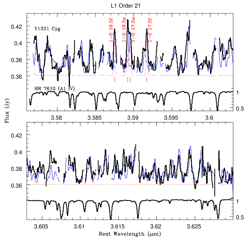
Figure 2a: A rich infrared spectrum is observed in V1331 Cyg (upper thick histogram, both panels) arising from emission by numerous water lines blended with OH lines (vertical red ticks, labeled). We model the emission across multiple $L$-band orders (Figs. 2a–2h), and find a good model fit (solid blue line) to the data by combining H₂O (dashed blue line) and OH (dotted red line) model spectra synthesized at $T=1500$ K with different column densities ($2\times 10^{21}$ and $1\times 10^{20}\rm\,cm^{-2}$, respectively) and disk emitting areas (5.5 $<R_{\rm H_{2}O}/R_{\odot}<19$ and 5.5 $<R_{\rm OH}/R_{\odot}<28$, respectively). Telluric absorption is indicated by the spectrum of the hot star, HR 7610 (lower thick histogram, both panels). Wavelength regions in the data and models where the telluric transmission is below 80% are not plotted. (A color version of the figure is available in the online journal)

Figure 2b: As in Fig. 2a but for the L2 order 21 wavelength region.

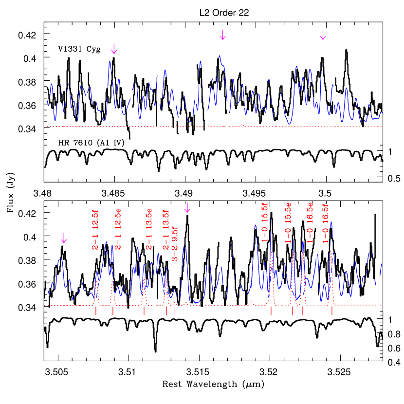
Figure 2c: As in Fig. 2a but for the L2 order 22 wavelength region. The OH line emission (red ticks, lower panel) is strong and optically thick, characterized by $\nu$ = 2–1 and 1–0 lines (see Table 1). While the combined H₂O+OH emission model (solid blue) fits much of the observed structure well, some wavelength offsets between the reference model and the data are discernible (vertical arrows) along with discrepancies in the strengths of some line groups. The vertical arrows illustrate some examples of water lines in this order that may need empirical adjustments to their theoretically computed transition wavelengths and/or oscillator strengths in the BT2 line list (see $\S$3.2).

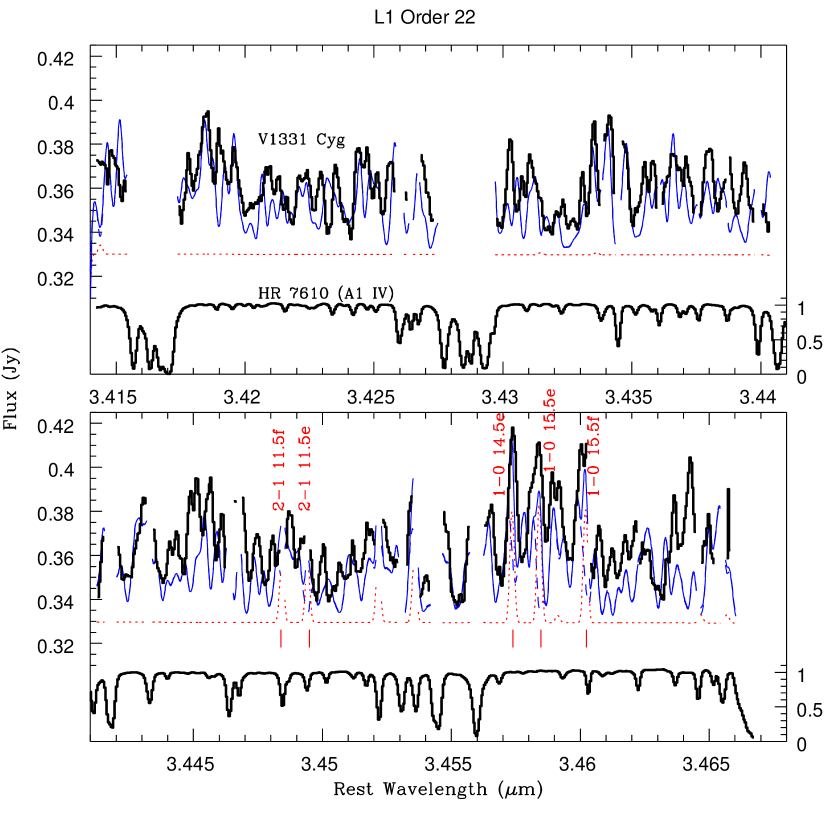
Figure 2d: As in Fig. 2a but for the L1 order 22 wavelength region.

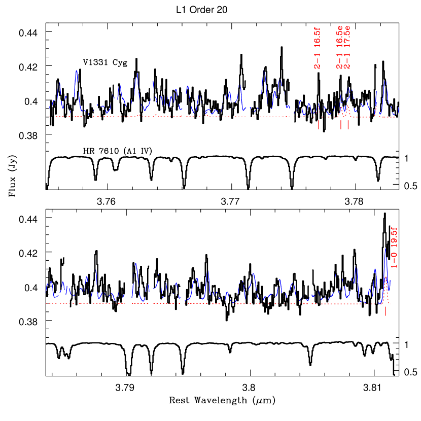
Figure 2e: As in Fig. 2a but for the L1 order 20 wavelength region.

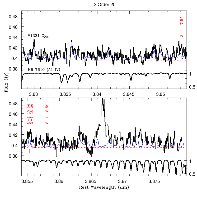
Figure 2f: As in Fig. 2a but for the L2 order 20 wavelength region. We observe an unknown strong emission feature at 3.8667 $\mu$m, which could be identified as a Mg I line ($\lambda_{\rm rest}=3.86748~{}\mu$m) that is blue shifted by 60 ${\rm km}\,{\rm s}^{-1}$ relative to the disk emission we detect, perhaps as part of an outflowing wind.

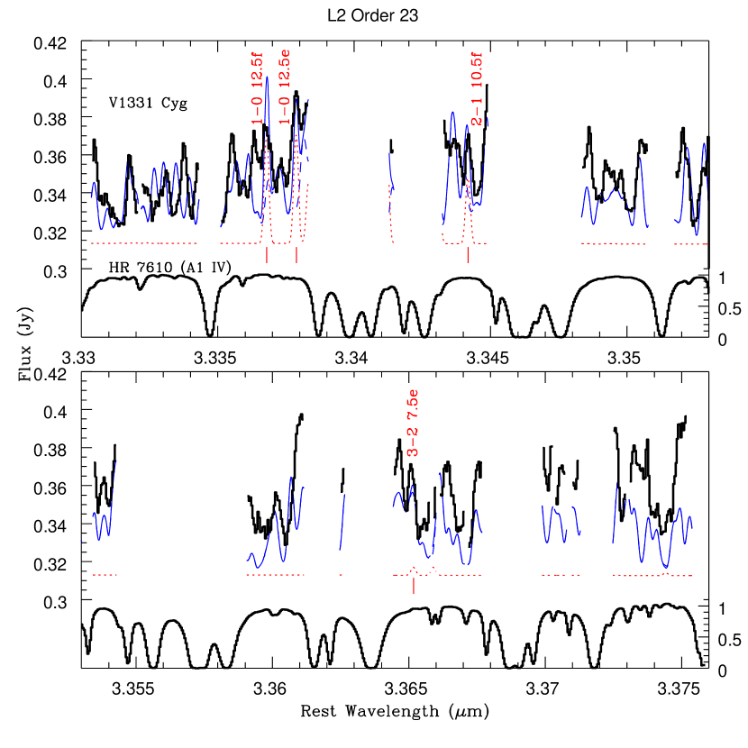
Figure 2g: As in Fig. 2a but for the L2 order 23 wavelength region.

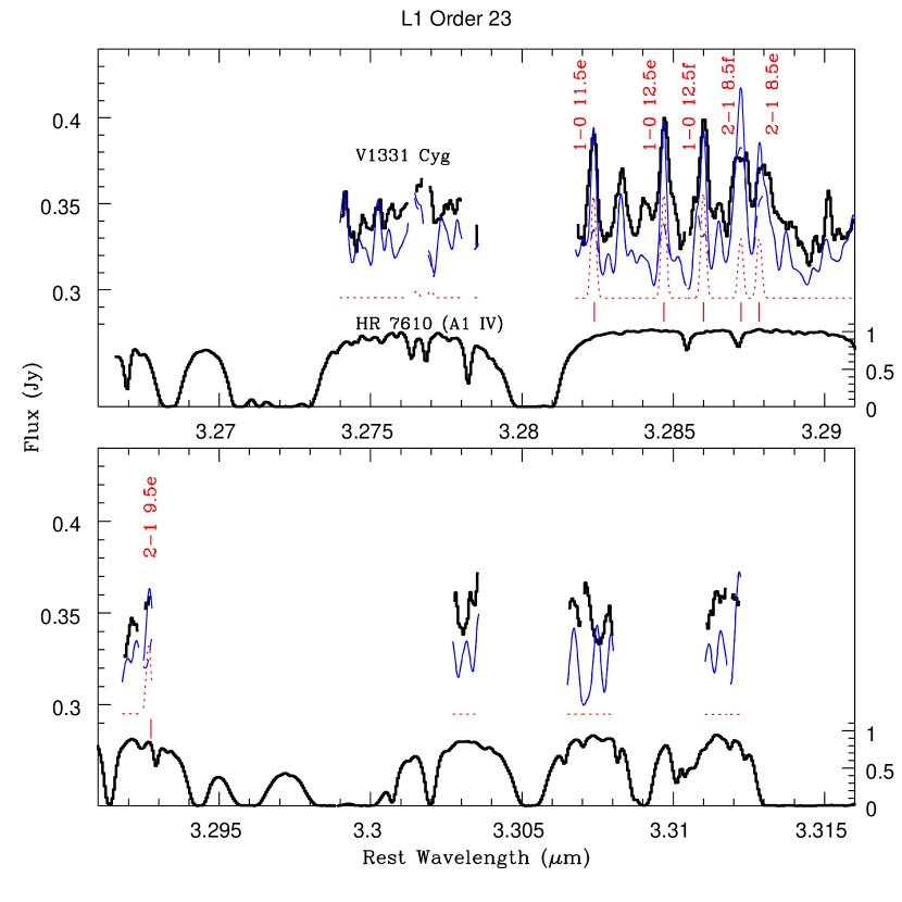
Figure 2h: As in Fig. 2a but for the L1 order 23 wavelength region.

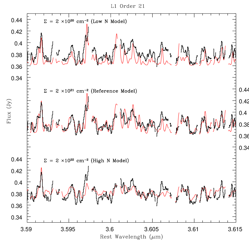
Figure 3a: Model fits of water emission to the data in a portion of the L1 order 21 region with different column density and emitting area values for a fixed temperature ($T=1500\,$K). The emitting area was chosen to optimize the fit to the model flux level in this order. The low column density case ($N_{\rm H_{2}O}$=$2.0\times 10^{20}\rm\,cm^{-2},R_{\rm out}=43R_{\odot}$, thin red line top panel) shows a poor fit to the data (black histogram), having too much contrast between the strengths of the strong and weak lines, indicating that the lines are too optically thin. In the high column density case ($N_{\rm H_{2}O}$=$2.0\times 10^{22}\rm\,cm^{-2},R_{\rm out}=12R_{\odot}$, thin red line lower panel), the fit to the data is also poor because the strong and weak lines do not show enough contrast, since they are much more optically thick. The center panel shows a good fit to the data ($N_{\rm H_{2}O}$=$2.0\times 10^{21}\rm\,cm^{-2},R_{\rm out}=19R_{\odot}$) having a mix of optically thin and thick lines that reproduce the strengths of both the strong and weak lines in this order.

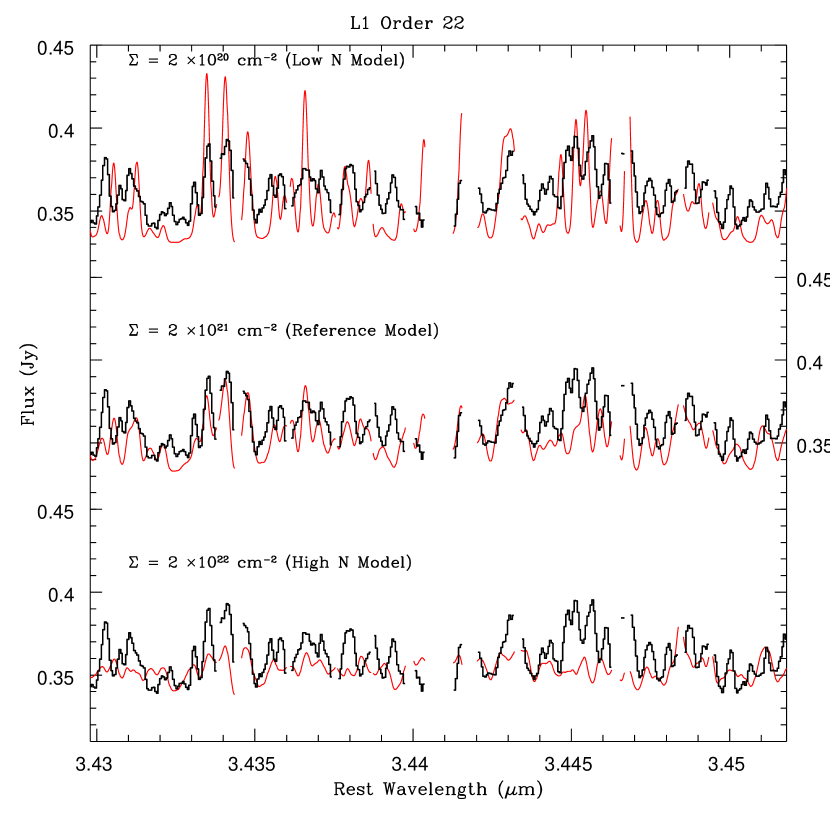
Figure 3b: As in Fig. 3a but for a portion of the L1 order 22 region. The high and low column density models fit the data more poorly here (compared to Fig. 3a) because the assumed emitting area is that chosen to optimize the fit to L1 order 21.

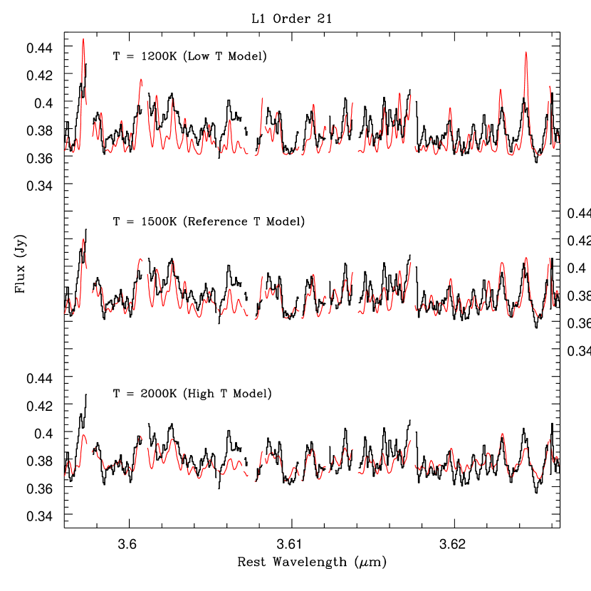
Figure 4a: Model fits of water emission to the data in a portion of the L1 order 21 region with temperature and emitting area values for a fixed column density ($N=2\times 10^{21}\rm\,cm^{-2}$). The low temperature case ($T=1200K,R_{\rm out}=35R_{\odot}$, thin red line top panel ) shows a poor fit to the data (thick black histogram), with the contrast between strengths of the strong and weak lines being too great. In the high temperature case ($T=2000K,R_{\rm out}=11R_{\odot}$, thin red line lower panel), the fit to the data is also poor because the strong and weak lines do not show enough contrast. The center panel shows a good fit to the data ($T=1500K,R_{\rm out}=19R_{\odot}$).

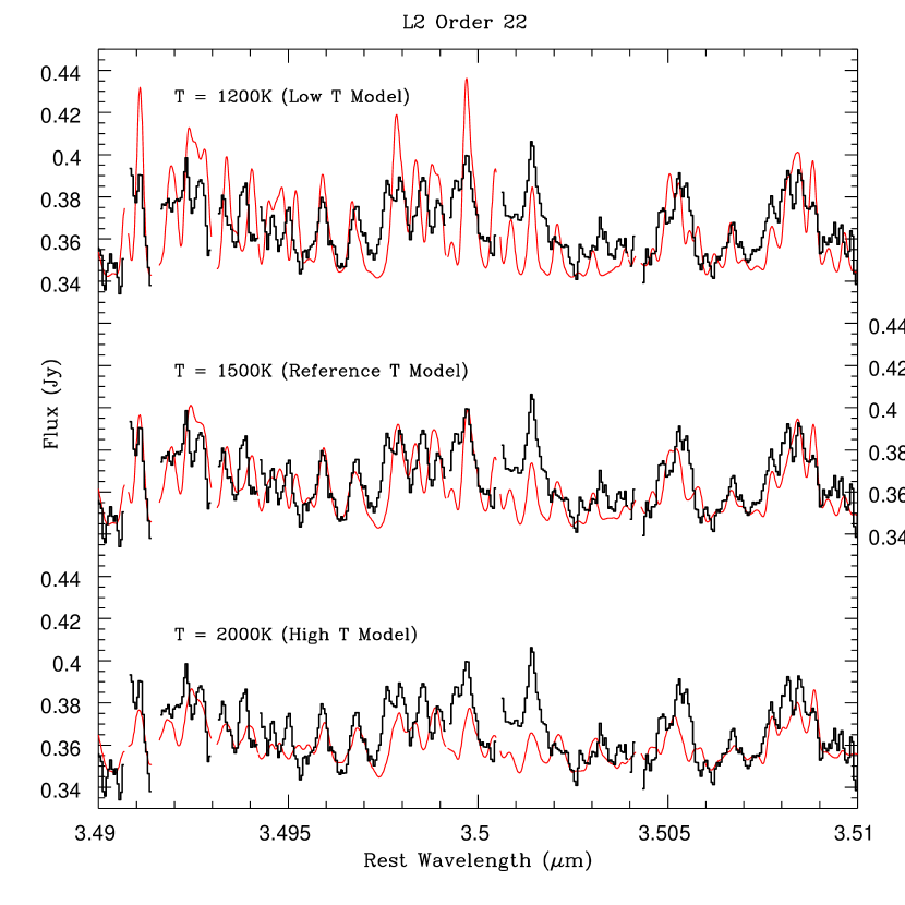
Figure 4b: As in Fig. 4a but for a portion of the L2 order 22 region.

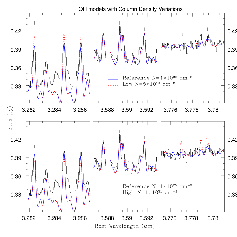
Figure 5a: OH model fits for higher and lower column densities than the reference OH model at a fixed temperature (T=1500 K) compared with the observed V1331 Cyg spectrum (black histogram). The top panel compares the reference OH model (N=$1\times 10^{20}\rm\,cm^{-2}$, solid blue line) with a low column density model (N=$5\times 10^{19}\rm\,cm^{-2}$; dotted red line). The low column density model overpredicts the flux of the lines at shorter wavelengths (3.282-3.287 $\mu$m). The bottom panel compares the reference model (N=$1\times 10^{20}\rm\,cm^{-2}$, solid blue line) with a high column density model (N=$1\times 10^{21}\rm\,cm^{-2}$, dotted red line). The high column density model underpredicts the flux of the lines at shorter wavelengths (3.282-3.287 $\mu$m) and somewhat overpredicts the flux of the lines at longer wavelengths (3.776-3.780 $\mu$m). The reference model fits all the OH lines (vertical ticks, see Table 1) adequately well across a range of optical depths.

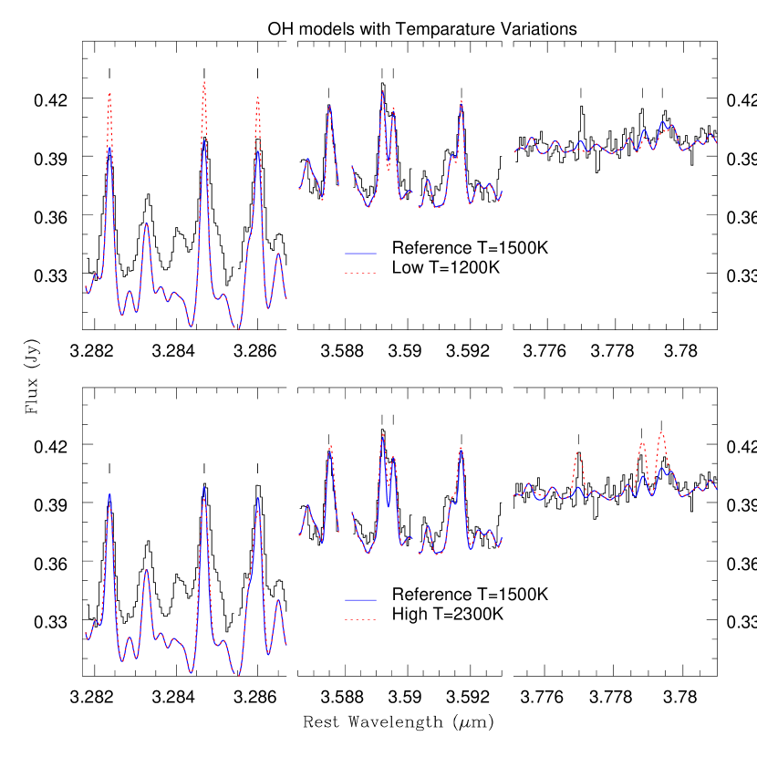
Figure 5b: OH model fits for higher and lower temperatures than the reference OH model at a fixed column density (N= $1\times 10^{20}\rm\,cm^{-2}$) compared with the observed V1331 Cyg spectrum (black histogram). The top panel compares the reference OH model (T=1500 K, solid blue line) with a low temperature model (T=1200 K; dotted red line). The low temperature model overpredicts the flux of the low-J lines at shorter wavelengths (3.282-3.287 $\mu$m). The bottom panel compares the reference model (T=1500 K, solid blue line) with a high temperature model (T=2300 K, dotted red line). The high temperature model overpredicts the flux of the high-J lines at longer wavelengths (3.776-3.780 $\mu$m). The low temperature model puts too much energy into the low-J lines (shorter wavelengths, top panel), and the high temperature model puts too much energy into the high-J lines (longer wavelengths, bottom panel). The reference model fits all the OH lines (vertical ticks, see Table 1) adequately well across a range of excitation levels.

Table 1: Physical properties of OH lines detected in our observations

$L$-band Order	Transition $\lambda$($\rm\AA$)	Line Transition Details	Model Line Opacity
L1 order 23	32823.671	$\nu$=1-0; J=11.5e	22.9
	32846.868	$\nu$=1-0; J=12.5e	26.0
	32859.990	$\nu$=1-0; J=12.5f	25.8
	32872.299	$\nu$=2-1; J=8.5f	2.5
	32878.437	$\nu$=2-1; J=8.5e	2.5
	32926.693	$\nu$=2-1; J=9.5e	2.9
L2 order 23	33367.886	$\nu$=1-0; J=12.5f	17.2
	33378.685	$\nu$=1-0; J=12.5e	17.0
	33441.684	$\nu$=2-1; J=10.5f	2.5
	33651.661	$\nu$=3-2; J=7.5e	0.16
L1 order22	34484.234	$\nu$=2-1; J=11.5f	1.4
	34494.249	$\nu$=2-1; J=11.5e	1.4
	34573.554	$\nu$=1-0; J=14.5e	8.4
	34584.036	$\nu$=1-0; J=15.5e	9.3
	34602.034	$\nu$=1-0; J=15.5f	9.2
L2 order 22	35077.159	$\nu$=2-1; J=12.5f	1.1
	35088.615	$\nu$=2-1; J=12.5e	1.1
	35110.880	$\nu$=2-1; J=13.5e	1.2
	35126.505	$\nu$=2-1; J=13.5f	1.2
	35132.676	$\nu$=3-2; J= 9.5f	0.11
	35201.132	$\nu$=1-0; J=15.5f	5.6
	35216.445	$\nu$=1-0; J=15.5e	5.5
	35223.349	$\nu$=1-0; J=16.5e	6.1
	35243.170	$\nu$=1-0; J=16.5f	6.0
L1 order 21	35874.842	$\nu$=1-0; J=16.5f	3.6
	35891.844	$\nu$=1-0; J=16.5e	3.5
	35895.358	$\nu$=1-0; J=17.5e	3.9
	35917.113	$\nu$=1-0; J=17.5f	3.8
L2 order 21	36582.769	$\nu$=1-0; J=17.5f	2.2
	36601.565	$\nu$=1-0; J=17.5e	2.2
	36601.815	$\nu$=1-0; J=18.5e	2.4
	36625.624	$\nu$=1-0; J=18.5f	2.4
L1 order 20	37788.009	$\nu$=2-1; J=16.5e	0.24
	37793.784	$\nu$=2-1; J=17.5e	0.27
	38109.260	$\nu$=1-0; J=19.5f	0.75
L2 order 20	38532.612	$\nu$=2-1; J=17.5f	0.16
	38552.724	$\nu$=2-1; J=17.5e	0.15
	38554.918	$\nu$=2-1; J=18.5e	0.17
	38580.509	$\nu$=2-1; J=18.5f	0.17

Table 2: Comparison of molecular gas parameters derived for V1331 Cyg

Obs. Date	$\lambda$	Molecule	$T$	$N$	Emitting Radii	$v_{\rm turb}$	$N_{\rm Mol}/N_{\rm H_{2}O}$
(UT)			(K)	($\times 10^{21}\rm\,cm^{-2}$)	($R_{\odot}$)	(${\rm km}\,{\rm s}^{-1}$)
1999 July 3	K	CO	1800	6	2.3 – 18	4	3–10
1999 July 3	K	H2O	1500	0.6	5.5 – 26	4	1
1999 July 3	K	H2O	1500	2	5.5 – 26	0	1
2001 July 11	L	H2O	1500	2	5.5 – 19	0	1
2001 July 11	L	OH	1500	0.1	5.5 – 28	0	0.05

References

- Agúndez et al. (2008) Agúndez, M., Cernicharo, J., & Goicoechea, J. R. 2008, A&A, 483, 831
- Alves et al. (1998) Alves, J., Lada, C. J., Lada, E. A., Kenyon, S. J., & Phelps, R. 1998, ApJ, 506, 292
- Balbus & Hawley (1991) Balbus, S. A., & Hawley, J. F. 1991, ApJ, 376, 214
- Bethell & Bergin (2009) Bethell, T., & Bergin, E. 2009, Science, 326, 1675
- Barber et al. (2006) Barber, R. J., Tennyson, J., Harris, G. J., & Tolchenov, R. N. 2006, MNRAS, 368, 1087 (BT2)
- Branham (1982) Branham, R. L., Jr. 1982, AJ, 87, 928
- Carr (1989) Carr, J. S. 1989, ApJ, 345, 522
- Carr et al. (2004) Carr, J. S., Tokunaga, A. T., & Najita, J. 2004, ApJ, 603, 213
- Carr & Najita (2008) Carr, J. S., & Najita, J. R. 2008, Science, 319, 1504
- Carr & Najita (2011) Carr, J. S., & Najita, J. R. 2011, accepted
- Chavarría (1981) Chavarría, C. 1981, A&A, 101, 105
- Eisner et al. (2007) Eisner, J. A., Hillenbrand, L. A., White, R. J., Bloom, J. S., Akeson, R. L., & Blake, C. H. 2007, ApJ, 669, 1072
- Fedele et al. (2011) Fedele, D., Pascucci, I., Brittain, S., Kamp, I., Woitke, P., Williams, J. P., Dent, W. R. F., & Thi, W. -. 2011, arXiv:1103.6039
- Glassgold et al. (2004) Glassgold, A. E., Najita, J., & Igea, J. 2004, ApJ, 615, 972
- Glassgold et al. (2009) Glassgold, A. E., Meijerink, R., & Najita, J. R. 2009, ApJ,701, 142
- Hamann & Persson (1992) Hamann, F., & Persson, S. E. 1992, ApJ, 394, 628
- Herbig & Dahm (2006) Herbig, G. H., & Dahm, S. E. 2006, AJ, 131, 1530
- Kamp et al. (2005) Kamp, I., Jonkheid, B., Augereau, J.-C., & van Dishoeck, E. 2005, Nearby Resolved Debris Disks, 15
- Knez et al. (2007) Knez, C., et al. 2007, BAAS, 38, 812
- Kuhi (1964) Kuhi, L. V. 1964, Ph.D. Thesis
- Levreault (1988) Levreault, R. M. 1988, ApJ, 330, 897
- Mandell et al. (2008) Mandell, A. M., Mumma, M. J., Blake, G. A., Bonev, B. P., Villanueva, G. L., & Salyk, C. 2008, ApJ, 681, L25
- McLean et al. (1998) McLean, I. S. et al. 1998, Proc. SPIE, 3354, 566
- Massey et al. (1992) Massey, P., Valdes, F., Barnes, J. 1992 A Users’s Guide to Reducing Slit Spectra with IRAF, National Optical Astronomy Observatory
- Massey et al. (1997) Massey, P. 1997 A User’s Guide to CCD reductions with IRAF, National Optical Astronomy Observatory
- McMuldroch (1993) McMuldroch, S., Sargent, A. I., & Blake, G. A. 1993, AJ, 106, 2477
- Najita et al. (1996) Najita, J., Carr, J. S., Glassgold, A. E., Shu, F. H., & Tokunaga, A. T. 1996, ApJ, 462, 919
- Najita et al. (2000) Najita, J. R., Edwards, S., Basri, G., & Carr, J. 2000, Protostars and Planets IV, 457
- Najita et al. (2003) Najita, J., Carr, J. S., & Mathieu, R. D. 2003, ApJ, 589, 931
- Najita et al. (2007) Najita, J. R., Carr, J. S., Glassgold, A. E., & Valenti, J. A. 2007, Protostars and Planets V, 507
- Najita et al. (2009) Najita, J. R., Doppmann, G. W., Carr, J. S., Graham, J. R., & Eisner, J. A. 2009, ApJ, 691, 738
- Partridge & Schwenke (1997) Partridge, H., & Schwenke, D. 1997, J. Chem. Phys., 106, 4618 (PS)
- Pontoppidan et al. (2005) Pontoppidan, K. M., Dullemond, C. P., van Dishoeck, E. F., Blake, G. A., Boogert, A. C. A., Evans, N. J., II, Kessler-Silacci, J. E., & Lahuis, F. 2005, ApJ, 622, 463
- Pontoppidan et al. (2008) Pontoppidan, K. M., et al. 2008, ApJ, 678, 1005
- Pontoppidan et al. (2010a) Pontoppidan, K. M., Salyk, C., Blake, G. A., Meijerink, R., Carr, J. S., & Najita, J. 2010, ApJ, 720, 887
- Pontoppidan et al. (2010b) Pontoppidan, K. M., Salyk, C., Blake, G. A., Käufl, H. U. 2010, ApJ, 722, L173
- Rothman et al. (1998) Rothman, L. S., et al. 1998, J. Quant. Spec. Radiat. Transf., 60, 665
- Salyk et al. (2011) Salyk, C., Pontoppidan, K. M., Blake, G. A., Najita, J. R., & Carr, J. S. 2011, arXiv:1104.0948 Salyk, C., et al. ApJ, submitted 2011
- Salyk et al. (2008) Salyk, C., Pontoppidan, K. M., Blake, G. A., Lahuis, F., van Dishoeck, E. F., & Evans, N. J., II 2008, ApJ, 676, L49
- Shevchenko et al. (1991) Shevchenko, V. S., Yakulov, S. D., Hambarian, V. V., & Garibjanian, A. T. 1991, AZh, 68, 275
- Sturm et al. (2010) Sturm, B., et al. 2010, A&A, 518, L129
- Thi & Bik (2005) Thi, W.-F., & Bik, A. 2005, A&A, 438, 557
- van Dishoeck & Dalgarno (1984) van Dishoeck, E. F., & Dalgarno, A. 1984, Icarus, 59, 305
- Willacy & Woods (2009) Willacy, K., & Woods, P. M. 2009, ApJ, 703, 479
- Yoshino et al. (1996) Yoshino, K., Esmond, J. R., Sun, Y., Parkinson, W. H., Ito, K.,& Matsui, T. 1996, J. Quant. Spec. Radiat. Transf., 55, 53