All scale-free networks are sparse

Abstract

We study the realizability of scale free-networks with a given degree sequence, showing that the fraction of realizable sequences undergoes two first-order transitions at the values 0 and 2 of the power-law exponent. We substantiate this finding by analytical reasoning and by a numerical method, proposed here, based on extreme value arguments, which can be applied to any given degree distribution. Our results reveal a fundamental reason why large scale-free networks without constraints on minimum and maximum degree must be sparse.

Many complex systems can be modeled as networks, i.e., as a set of connections (edges) linking discrete elements (nodes) Alb02 ; New03 ; Boc06 . A characteristic of a network that affects many physical properties is its degree distribution $P\left(k\right)$, the probability of finding a node with $k$ edges. Considerable attention has been paid to scale-free networks, in which the degree distribution follows a power-law, $P\left(k\right)\sim k^{-\gamma}$ Cal07 ; Pri65 ; Red98 ; AlbXX ; AmaXX ; New01 ; Vaz02 . In particular, scale-freeness has been shown to have important implications in the thermodynamic limit. For studying the properties of scale-free networks, several generative models have been proposed Alb02 ; New03 ; Boc06 ; Cal07 . However, no models creating networks with $\gamma<2$ have been found Dor00 ; Kra00 , and $\gamma<2$ is observed only in networks that are relatively small or in which the power-law behavior has some cutoff New01 . In this Letter, we explain the absence of large networks that exhibit a power-law with $0<\gamma<2$ in the tail of the distribution. Specifically, we show that fundamental constraints exist that prevent the realization of any such network.

It is well known that the mean degree of scale-free distributions with exponents $\gamma$ less than 2 diverges in the thermodynamic limit, i.e., when the number of nodes $N\rightarrow\infty$ New03 . Scale-free networks with $\gamma<2$ would therefore be called dense networks, whereas networks $\gamma>2$ are sparse. While sparseness is a common property, which is regularly exploited in data storage and algorithms, also many examples of dense networks are known Spi03 ; Ton04 ; Hag08 . It is thus reasonable to ask why there are no examples of dense scale-free networks. We answer this question by showing that dense networks with a power-law degree distribution must have $\gamma<0$. Calling such networks scale-free is at best dubious because they would not exhibit the characteristic properties commonly associated with scale-freeness for $N\rightarrow\infty$.

The absence of dense scale-free networks is explained by a discontinuous transition in the realizability of such networks. Below, we show numerically, analytically, and by a hybrid method proposed here, that the probability of finding a scale free-network with a given $\gamma$ is 0 for $0<\gamma<2$. We emphasize that these results are not contingent on a specific generative model, but arise directly from fundamental mathematical constraints.

The generation of scale-free networks with a given degree distribution can be considered as a two-step procedure. First, one creates a number of nodes and assigns to each node a number of connection “stubs” drawn from the degree distribution. The realization of the degree distribution that is thus created is called degree sequence. Second, one connects the stubs such that every stub on a given node links to a stub on a different node, without forming self-loops or double links. However, not every degree sequence can be realized in a network. Sequences that admit realizations as simple graphs are called graphical, and their realizability property is commonly referred to as graphicality Erd60 . Graphicality fails trivially if the number of stubs is odd, as one needs two stubs to form every link, or if the degree of any node is equal to or greater than the number of nodes, as it would be impossible to connect all its stubs to different nodes. Below we do not consider sequences for which graphicality is such trivially violated, but note that further conditions must be met for a sequence to be graphical Kim09 ; Del10 .

The main result used for testing the graphicality of a degree sequence is the Erdős-Gallai theorem, stated here as reformulated in Del10 using recurrence relations:

Theorem 1.

Let $\mathcal{D}=\left\{d_{0},d_{1},\dotsc,d_{N-1}\right\}$ be a non-increasing degree sequence on $N$ nodes. Define $x_{k}=\min\left\{i:d_{i}<k+1\right\}$ and $k^{\star}=\min\left\{i:x_{i}<i+1\right\}$. Then, $\mathcal{D}$ is graphical if and only if $\sum_{i=0}^{N-1}d_{i}$ is even, and

$$L_{k}\leqslant R_{k}\quad\forall\>0\leqslant k<N-1\>,$$ (1)

where $L_{k}$ and $R_{k}$ are given by the recurrence relations

$$L_{0} =d_{0}$$ (2)

$$L_{k} =L_{k-1}+d_{k}$$ (3)

and

$$R_{0} =N-1$$ (4)

$$R_{k} =\left\{\begin{array}[]{ll}R_{k-1}+x_{k}-1&\forall k<k^{\star}\\ R_{k-1}+2k-d_{k}&\forall k\geqslant k^{\star}\end{array}\right.\>.$$ (7)

This formulation of the theorem has the advantage over the traditional one Erd60 of allowing a very fast implementation of a graphicality test Del10 .

Equivalently, graphicality can be tested by a recursive application of the Havel-Hakimi theorem Hav55 ; Hak62 :

Theorem 2.

A non-increasing degree sequence $\mathcal{D}=\left\{d_{0},d_{1},\dotsc,d_{N-1}\right\}$ is graphical if and only if the sequence $\mathcal{D}^{\prime}=\left\{d_{1}-1,d_{2}-1,\dotsc,d_{d_{0}}-1,\dotsc,d_{N-1}\right\}$ is graphical.

To investigate the dependence of the graphicality of scale-free networks on the power-law exponent $\gamma$, we performed extensive numerics, generating ensembles of sequences of random power-law distributed integers with range between 1 and $N-1$ and $\gamma$ between $−2$ and 4. We tested each sequence for graphicality by applying Th. 1, and computed for each $\gamma$ the graphical fraction

$$g=\frac{G}{E}\>,$$

where $G$ is the total number of graphical sequences in the ensemble and $E$ is the number of sequences in the ensemble with an even degree sum. The results, plotted in Fig. 1, clearly show two graphicality transitions: For very large and very small exponents almost all sequences are graphical. However, at intermediate exponents there is a pronounced gap where almost no sequence is graphical. The transitions between the two phases become steeper and the transition points approach $\gamma=0$, and $\gamma=2$ as the system size is increased.

The dependence of $g$ on sequence length strongly suggests that both transitions are first-order. To verify their character, we studied Binder’s cumulants $U_{4}\equiv 1-\left\langle g^{4}\right\rangle/{\left\langle g^{2}\right\rangle}^{2}$ Bin81 ; Bin81_2 . For continuous transitions, the cumulants for different system sizes lie within a finite interval and cross at the critical point, whereas for first-order transitions the curves are flat, except for a diverging negative minimum whose position converges to the transition point with increasing system size Bin84 ; Vol93 ; Lan00 . In the present system the cumulants confirm that the graphicality transitions at $\gamma=0$ and $\gamma=2$ are first order.

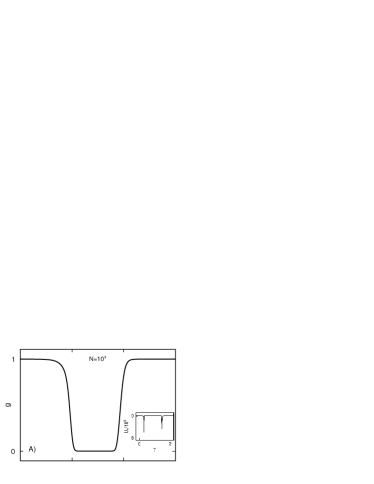
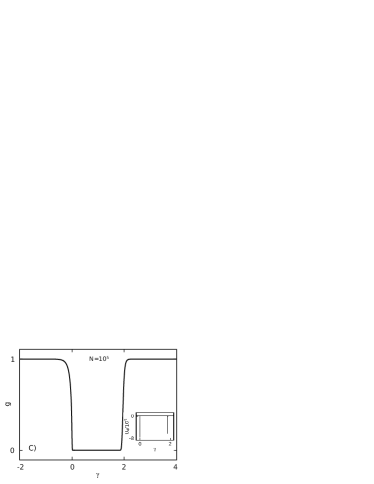
Figure 1: Graphicality transitions in scale-free networks. The plots of graphical fraction $g$ vs. exponent $\gamma$ show transitions at $\gamma=0$ and $\gamma=2$. Binder’s cumulants, in the insets, identify the character of the transitions and the transition points.

To understand the origin of the transitions, we focus on the scaling of the largest degrees and of the number of lowest degree nodes in the sequences. Below, we show that the first two largest degrees are of order $O\left(N\right)$ for $\gamma\leqslant 2$, while they grow sublinearly with $N$ for $\gamma>2$. Also, the number of nodes with degree of order $O\left(1\right)$ increases linearly with $N$ for $\gamma\geqslant 0$ and decreases like $N^{\gamma}$ for $\gamma<0$. Then, the transitions can be understood as follows: If we tried to construct a scale-free network with $\gamma$ between 0 and 2, following the Havel-Hakimi algorithm, $O\left(N\right)$ nodes with unitary degree would be used to place the connections involving the first node, and then there would be no way to place all the needed edges involving the node with the second largest degree. Conversely, when $\gamma<0$, all but a vanishingly small fraction of nodes have a degree of order $O\left(N\right)$, and for $N\rightarrow\infty$ all the nodes are able to form as many connections as needed.

To see this, calculate the expected maximum degree of a scale-free sequence

$$\widehat{d}=\max\left\{x:\ N\sum_{k=x}^{N-1}\frac{k^{-\gamma}}{H_{N-1,\gamma}}\geqslant 1\right\}\>,$$ (8)

where $H_{a,b}$ is the $a^{\mathrm{th}}$ generalized harmonic number of exponent $b$

$$H_{a,b}=\sum_{t=1}^{a}t^{-b}\>.$$

When $N\gg 1$, Eq. 8 becomes

$$N\int_{x}^{N-1}\frac{k^{-\gamma}}{H_{N-1,\gamma}}\mathrm{dk}=1\>.$$ (9)

Because of the dependence of the behavior of the generalized harmonic number on the exponent, we solve this equation for different values of $\gamma$.

Solving the integral for $\gamma>1$ gives

$$\frac{N}{\left(1-\gamma\right)H_{N-1,\gamma}}\left[\left(N-1\right)^{1-\gamma}-x^{1-\gamma}\right]=1\>.$$ (10)

Equation 10, for $N\gg 1$ implies

$$x=\left[\frac{N}{\left(\gamma-1\right)H_{N-1,\gamma}}\right]^{\frac{1}{\gamma-1}}\sim N^{\frac{1}{\gamma-1}}\>.$$

Because of the upper bound of the degrees of a sequence at $N-1$, if $1<\gamma\leqslant 2$, the value of the largest degree grows linearly with the number of nodes $N$.

For $\gamma=1$, the integral in Eq. 9 gives

$$\log\left(N-1\right)-\log\left(x\right)=\frac{H_{N-1}}{N}\>,$$

where $H_{N-1}=H_{N-1,1}$ is the $\left(N-1\right)^{\mathrm{th}}$ harmonic number. To solve the above equation note that the right-hand side vanishes in the limit of large $N$. This can be seen by an application of l’Hôpital’s rule, noticing that for $\gamma\geqslant 0$

$$\frac{\partial}{\partial\mathrm{N}}H_{N-1,\gamma}=\gamma\left[\zeta\left(\gamma+1\right)-H_{N-1,\gamma+1}\right]$$

and

$$\lim_{N\rightarrow\infty}H_{N,\gamma}=\zeta\left(\gamma\right)\>,$$

where $\zeta$ is Riemann’s zeta function. Then, the solution of the equation in the thermodynamic limit is $x\sim N$.

Next, for $0\leqslant\gamma<1$, Eq. 9 yields Eq. 10, hence

$$\left(N-1\right)^{1-\gamma}-x^{1-\gamma}=\frac{\left(1-\gamma\right)H_{N-1,\gamma}}{N}\>.$$ (11)

As in the previous case, the right hand side vanishes for large $N$, and the solution is that $x\sim N$.

Finally, for $\gamma<0$, from Eq. 10 one gets again Eq. 11. However, in this case the right-hand side grows as $N^{-\gamma}$. Since $\gamma$ is negative, one can rewrite Eq. 11 for large $N$ as

$$\left(N-1\right)^{1+\left|\gamma\right|}-x^{1+\left|\gamma\right|}=N^{\left|\gamma\right|}\>,$$

which implies again that $x\sim N$.

The same arguments can be applied to the scaling of the second largest degree, with identical results. Now, consider the number $A$ of nodes with unitary degree. For large $N$, $A=N/H_{N-1,\gamma}$. Thus, when $\gamma\geqslant 0$, $A\sim N$, whereas, if $\gamma<0$, then $A\sim N^{\gamma}$.

Then, to formally check the transition mechanism, explicitly write inequality 1 for $k=1$. The left-hand-side consists of the sum of the largest and the second largest degrees, which can be obtained using the same argument as above. To compute the right hand side, first notice that $k^{\star}\geqslant 2$. In fact, by definition it cannot be 0, as this would imply that the highest degree in the sequence would be 0. Moreover, in our case it cannot be 1, as this would imply that the second highest degree in the sequence would be 1, in contradiction with what demonstrated above. Also, by the definition of $x_{k}$, it follows that $x_{1}=N-A$. Thus, applying Eq. 7, the right hand side is simply $2N-2-A$. Therefore, the inequality reads

$$\left[\frac{\left(\gamma-1\right)H_{N-1,\gamma}}{N}+\left(N-1\right)^{1-\gamma}\right]^{\frac{1}{1-\gamma}}+\left[\frac{2\left(\gamma-1\right)H_{N-1,\gamma}}{N}+\left(N-1\right)^{1-\gamma}\right]^{\frac{1}{1-\gamma}}\leqslant 2N-2-\frac{N}{H_{N-1,\gamma}}\>.$$ (12)

A numerical solution shows that for $N\gg 1$ the above inequality is indeed satisfied only when $\gamma<0$ or $\gamma>2$, confirming the transition mechanism. Notice, however, that when $N\rightarrow\infty$ almost all the nodes are fully connected for $\gamma<0$, and thus it is not appropriate to refer to such networks as scale-free.

One can also study the inequality in the presence of a cutoff in the distribution, by replacing every instance of the natural upper bound on the degrees, $\left(N-1\right)$, with the cutoff value. Cutoffs have been observed in real-world networks AmaXX ; New01 , and are sometimes imposed for different purposes, such as making the degree-degree correlations uniform Mos02 ; Cat05 . Notably, their effect is making the inequality always satisfied, and the transitions disappear.

The above treatment indicates that, by applying extreme value arguments, one can build a finite length sequence $S=\left\{s_{0},s_{1},\dotsc,s_{N-1}\right\}$ for the purpose of studying the graphicality of infinite systems. A finite sequence maximizing the degrees of the nodes for a given degree distribution will best approximate the graphicality of an infinite sequence, especially since broken graphicality is always caused by an excess of stubs in some subset of nodes. Therefore, for a length $N$, and any degree distribution $P\left(d\right)$, the elements of the sequence are given by the family of functionals

$$s_{i}=\max\left\{s^{\star}:N\sum_{d=s^{\star}}^{d_{M}}P\left(d\right)\geqslant i+1\right\}\>,$$ (13)

where $d_{M}$ is the largest allowed degree. In general, $d_{M}=N-1$, but the full generality of its value allows cutoffs to be accounted for. Increasing the number of nodes in the representative sequence will improve the accuracy in the determination of transition points, as it will better approximate an infinitely large system.

We computed degree maximizing sequences for power-law distributions, and tested them for graphicality. The results, shown in Fig. 2, are consistent with the simulations and with the analytical treatment, showing once again transitions at $\gamma=0$ and $\gamma=2$.

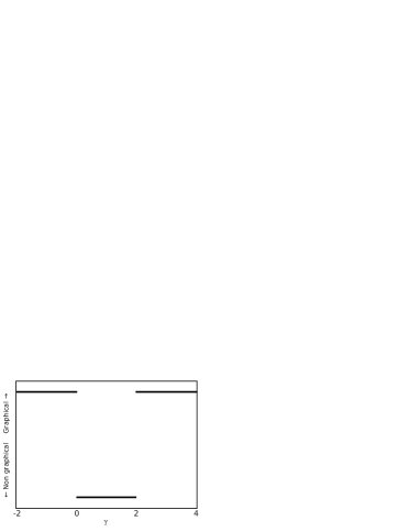
Figure 2: Graphicality of the degree maximizing sequence ($N=10^{6}$) given by Eq. 13 for scale-free distributions vs. exponent $\gamma$. The graphicality transitions points are correctly identified.

In conclusion, we showed that the graphicality of power-law degree sequences undergoes two discontinuous transitions at the values 0 and 2 of the exponent $\gamma$. In the limit of a large number of nodes, no network with an unbounded power-law degree distribution with $0<\gamma<2$ can exist. We emphasize that this result arises directly from mathematical constraints on the degrees of the nodes, and is thus independent of the specific procedure used for generating the network. It explains why the scale-free networks commonly observed in nature have $\gamma>2$ or have a cutoff. Established procedures may yield $0<\gamma<2$ when applied to data from a given finite network. However, when the network grows or more data is acquired either a cutoff must exist or $\gamma$ must increase above 2 (or decrease below 0). It is possible to generate large and dense networks with a power-law degree distribution with $\gamma<0$, but these networks should not be denoted as scale-free as they do not exhibit the properties that are commonly associated with scale-freeness. Any large scale-free network is thus sparse, either because $\gamma>2$ or because of the presence of a cutoff. This insight is reassuring as it implies that also numerical methods which are often needed for analyzing scale free networks will continue to scale favorably with increasing network size.

- (1) R. Albert and A.-L. Barabási, Rev. Mod. Phys. 74, 47 (2002).
- (2) M. E. J. Newman, SIAM Review 45, 167 (2003).
- (3) S. Boccaletti et al. Phys. Rep. 424, 175 (2006).
- (4) G. Caldarelli, Scale-free networks – complex webs in nature and technology (Oxford University Press, Oxford, United Kingdom, 2007).
- (5) D. J. de Solla Price, Science 149, 510 (1965).
- (6) S. Redner, Eur. J. Phys. B 4, 131 (1998).
- (7) R. Albert, H. Jeong, and A.-L. Barabási, Nature 401, 130 (1999); H. Jeong et al. Nature 407, 651 (2000); H. Jeong et al. Nature 411, 41 (2001).
- (8) L. A. N. Amaral et al. Proc. Natl. Acad. Sci. USA 97, 11149 (2000); F. Liljeros et al. Nature 411, 907 (2001).
- (9) M. E. J. Newman, Proc. Natl. Acad. Sci. USA 98, 404 (2001).
- (10) A. Vázquez, R. Pastor-Satorras, and A. Vespignani, Phys. Rev. E 65, 066130 (2002).
- (11) S. N. Dorogovtsev, J. F. F. Mendes, and A. N. Samukhin, Phys. Rev. Lett. 85, 4633 (2000).
- (12) P. L. Krapivsky, S. Redner, and F. Leyvraz, Phys. Rev. Lett. 85, 4629 (2000).
- (13) V. Spirin and L. A. Mirny, Proc. Natl. Acad. Sci. USA 100, 12123 (2003).
- (14) A. H. Y. Ton et al. Science 303, 808 (2004).
- (15) P. Hagmann et al. PLoS Biology 6, 1479 (2008).
- (16) H. Kim et al. J. Phys. A – Math. Theor. 42, 392001 (2009).
- (17) C. I. Del Genio et al. PLoS One 5, e10012 (2010).
- (18) P. Erdős and T. Gallai, Mat. Lapok 11, 477 (1960).
- (19) V. Havel, Časopis Pěst Mat 80, 477 (1955).
- (20) S. L. Hakimi, J. Soc. Ind. Appl. Math. 10, 496 (1962).
- (21) K. Binder, Z. Phys. B – Cond. Mat. 43, 119 (1981).
- (22) K. Binder, Phys. Rev. Lett. 47, 693 (1981).
- (23) K. Binder and D. P. Landau, Phys. Rev. B 30, 1477 (1984).
- (24) K. Vollmayr et al. Z. Phys. B 91, 113 (1993).
- (25) D. P. Landau and K. Binder, A guide to Monte Carlo simulations in statistical physics (Cambridge University Press, Cambridge, United Kingdom, 2000).
- (26) S. Mossa et al. Phys. Rev. Lett. 88, 138701 (2002).
- (27) M. Catanzaro, M. Boguñá, and R. Pastor-Satorras, Phys. Rev. E 71, 027103 (2005).