Critical Casimir forces for Ising films with variable boundary fields

Abstract

Monte Carlo simulations based on an integration scheme for free energy differences is used to compute critical Casimir forces for three-dimensional Ising films with various boundary fields. We study the scaling behavior of the critical Casimir force, including the scaling variable related to the boundary fields. Finite size corrections to scaling are taken into account. We pay special attention to that range of surface field strengths within which the force changes from repulsive to attractive upon increasing the temperature. Our data are compared with other results available in the literature.

I Introduction

Forces induced by thermal fluctuations can be very sensitive to tiny changes in temperature. This is exemplified by effective forces arising between two surfaces confining a fluid close to its critical point, for which a slight variation in temperature can lead to pronounced changes in their range and magnitude. The universal features of these so-called critical Casimir forces are captured by scaling functions FdG ; krech:99:0 ; dantchev ; they have been studied theoretically and experimentally for systems belonging to the bulk universality classes of the $XY$ and the Ising model krech:99:0 ; dantchev ; gambassi . The $XY$ model describes quantum fluids, such as liquid ⁴He close to its normal-superfluid phase transition or a ³He-⁴He mixture close to its tricritical point, whereas, e.g., a classical binary liquid mixture near its demixing point or a simple fluid close to a liquid-gas critical point belong to the Ising universality class.

In the systems studied so far experimentally, the measured critical Casimir forces have been either attractive or repulsive throughout the whole temperature range. (The addition of salt to a critical oil-water mixture presents a notable exception in that, under favorable conditions, on route to the critical demixing point the sign of the critical Casimir force can change twice soft_matter due to a coupling between the noncritical charge density and the critical order parameter field.) Here, we investigate simple systems which provide the possibility of changing the sign of the critical Casimir forces upon varying the temperature. Analytic studies and computer simulations indicate that the sign of the critical Casimir force is determined by the properties of the confining surfaces, i.e., by the boundary conditions (BCs) which they impose on the fluctuations of the order parameter characterizing the underlying second-order phase transition. Indirect measurements of the Casimir scaling function, inferred from wetting films of superfluids garcia ; garcia1 and of classical binary liquid mixtures pershan ; rafai , are consistent with these predictions. For pure ⁴He one has symmetric Dirichlet-Dirichlet $(O,O)$ BCs because the quantum mechanical wave function of the superfluid state vanishes at both confining interfaces. This gives rise to attractive critical Casimir forces EPL ; PRE ; hucht ; kardar ; LGW-MF . For wetting films of ³He-⁴He mixtures, $(+,O)$ BCs are realized because due to quantum mechanical effects a ⁴He-rich layer forms near the solid-liquid interface and favors the superfluid phase giving rise to the so-called surface transition LGW-MF ; MD_EPL ; $(+)$ indicates a symmetry-breaking BC with the surface completely ordered. Upon reaching the surface transition the superfluid order parameter becomes nonzero at the solid surface whereas it vanishes at the fluid-vapor interface of the wetting film. These asymmetric BCs give rise to a repulsive Casimir force. Measurements for wetting films of certain classical binary liquids mixtures have been found to be in agreement with $(+-)$ BCs corresponding to a strong opposing preferential adsorption of the two species of the mixture at the two confining surfaces krech ; EPL ; PRE ; upton . Within the framework of an Ising magnet (which is equivalent to the lattice model of a binary mixture) or within the continuum field theory for the order parameter, this amounts to the presence of strong antagonistic symmetry-breaking surface fields ${\bar{H}}_{1}$ and ${\bar{H}}_{2}$ which couple linearly to the order parameter and give rise to repulsive critical Casimir forces. Direct evidences for critical Casimir forces have been provided by studying the Brownian motion of a single colloidal particle near a flat substrate surface and immersed in the binary liquid mixture of water and lutidine Hertlein ; PRE_nature . The experimental results for the cases in which the colloid and the substrate surface preferentially adsorb the same species of the mixture are consistent with $(++)$ or $(--)$ BCs, whereas for cases in which the particle and the surface preferentially adsorb different species of the mixture the results agree with the occurrence of $(-+)$ or $(+-)$ BCs. Whereas the theoretical and experimental understanding of critical Casimir forces in the presence of strong or vanishing surface fields has reached a mature level, here we set out to study the influence of variable weak surface fields.

Dirichlet and $(\pm)$ BCs are the renormalization-group fixed-point boundary conditions corresponding to the so-called ordinary surface universality class $(O)$ and the normal transition surface universality class, respectively binder:83:0 ; diehl:86:0 ; diehl:97 . The ordinary transition corresponds to the bulk phase transition occurring in the absence of surface fields and with a reduced tendency to order at the surface. Within a mean field picture the latter is described by a surface scaling field $c$ so that $1/c$ plays the role of an extrapolation length of the order parameter profile; $c=\infty$ defines the ordinary transition fixed point. The normal transition occurs for systems with strong surface fields and which exhibit a reduced tendency to order if these surface fields are switched off. The normal transition is defined by the fixed point (${\bar{H}}_{1}=\infty,c=\infty$). As indicated by the nomenclature the normal transition is the generic situation for a fluid. In a spin model as discussed below $H_{1}={\bar{H}}_{1}/J$ is dimensionless with $J$ as an interaction constant (see below).

Near the ordinary transition there is a single linear scaling field $g_{1}=H_{1}/c^{y}$ associated with the surface field of strength $H_{1}$ and the surface enhancement parameter $c$ diehl:97 . The scaling exponent is $y=\left(\Delta_{1}^{sp}-\Delta_{1}^{ord}\right)/\Phi$, where $\Delta^{sp,ord}_{1}$ are the surface counterparts of the bulk gap exponent $\Delta$ and $\Phi$ is a crossover exponent binder:83:0 ; diehl:86:0 ; diehl:97 . For the three-dimensional $(D=3)$ Ising model one has $\Delta^{ord}_{1}\simeq 0.46(2)$ GZ , $\Delta_{1}^{sp}\simeq 1.05$ diehl:86:0 , $\Phi\simeq 0.68$ diehl:86:0 , and $y\simeq 0.87$; $\nu\simeq 0.63$ PV is the critical exponent of the bulk correlation length $\xi_{b}=\xi_{0}^{\pm}|t|^{-\nu}$ with the reduced temperature $t=(\beta_{c}-\beta)/\beta=(T-T_{c})/T_{c}$; $\pm$ corresponds to $t\gtrless 0$. The corresponding surface scaling variable can be chosen as $(\xi_{0}^{+})^{-y}g_{1}|t|^{-\Delta^{ord}_{1}}$. For $t\to 0$ the scaling variables tend to their fixed point values, and the scaling functions assume asymptotic forms corresponding to the respective fixed points diehl:86:0 ; diehl:97 . The scaling variable $|(\xi_{0}^{+})^{-y}g_{1}|t|^{-\Delta^{ord}_{1}}|^{\nu/\Delta^{ord}_{1}}$ is proportional to the ratio $\xi_{b}/\ell_{1}$ between the true bulk correlation length $\xi_{b}$ and the length $\ell_{1}$ introduced by the scaling field $g_{1}$:

$$\ell_{1}=\xi_{0}^{+}|(\xi_{0}^{+})^{-y}g_{1}|^{-\nu/\Delta_{1}^{ord}}.$$ (1)

The fixed point dominated critical regions correspond to either the divergence ( $(+)$ or $(-)$ fixed-point BCs) or the vanishing ( $(O)$ fixed-point BCs) of this ratio. The length $\ell_{1}$ corresponds to the range of distances from the surface within which the order parameter profile responds linearly to the presence of a surface field $H_{1}$ ritschel_czerner ; ciach_maciolek_stecki . (A precise definition of $\ell_{1}$ will be provided below.)

Depending on the interplay between $\ell_{1}$ and the length $\ell_{c}=(\xi_{0}^{+}c)^{-\nu/\Phi}$ associated with the surface enhancement parameter $c$ one finds various asymptotic regimes for the short-distance behavior $z\ll\xi_{b}$ of the order parameter profile diehl:97 ; ritschel_czerner ; ciach_ritschel . At the bulk critical point one has $\phi_{cri}(z)\sim g_{1}z^{\kappa}$ for distances $\ell_{c}\ll z\ll\ell_{1}$ from the surface with $\kappa=(\Delta_{1}^{ord}-\beta)/\nu$ and $\phi_{cri}(z)\sim z^{-\beta/\nu}$ for distances $\ell_{c}\ll\ell_{1}\ll z$ from the surface. We note that near the ordinary transition fixed-point (i.e., large $c$) the length $\ell_{c}$ is small whereas the length $\ell_{1}$ can be large or small. Within mean field theory one has $\kappa=0$ due to $\Delta_{1}^{ord}(D=4)=1/2$ and $\nu(D=4)=1/2$ whereas one has $\kappa(D=3)\simeq 0.23$ ritschel_czerner and $(\beta/\nu)(D=3)\simeq 0.52$ PV . Consequently, the critical order parameter (OP) profile turns out to be a nonmonotonic function of $z$. For $z\ll\ell_{1}$ the OP increases upon increasing $z$, at $z\simeq\ell_{1}$ it reaches a maximum and only for $z\gg\ell_{1}$ the universal ”normal“ fixed-point behavior, i.e., the decay of the OP occurs ritschel_czerner . Accordingly the position of this maximum can serve as a definition for the length $\ell_{1}$ ritschel_czerner ; ciach_maciolek_stecki . With increasing surface field strength the surface-near regime with the aforementioned increase $\sim z^{\kappa}$ of the OP becomes narrower, and eventually for $H_{1}\to\infty$ the length scale $\ell_{1}$ goes to zero, such that this regime disappears and the normal transition behavior $\sim z^{\beta/\nu}$ is attained throughout.

For the $2D$ Ising model on the square lattice with lattice constant $a$, the length $\ell_{1}$ has been extracted from an exact result for the scaling function of the OP profile below and above $T_{c}$; the profile at $T_{c}$ has not been reported. In the case that the exchange coupling between spins in the surface row is the same as in the bulk, the OP scaling function depends on the scaling variable $\xi_{b}/{\hat{l}}_{1}$ with ${\hat{l}}_{1}=(a/2)\tanh(K)/(\tanh{\bar{h}_{1}})^{2}$, where $K=J/(k_{B}T)$ is the dimensionless reduced exchange coupling between Ising spins and ${\bar{h}_{1}}={\bar{H}_{1}}/(k_{B}T)$ bariev . Thus for weak surface fields and in the limit $K\to K_{c}$, ${\hat{l}}_{1}(K_{c})=(a/2)K_{c}^{-2}\tanh(K_{c})/H_{1}^{2}=1.066(4)a{H_{1}}^{-2}=1.879(0)\xi_{0}^{+}H_{1}^{-2}$, where $K_{c}=0.5\ln(1+\sqrt{2})\simeq 0.44$ is the critical coupling and $\xi_{0}^{+}=a/(4K_{c})$. This is in line with Eq. (1) due to $\nu(D=2)=1$ and $\Delta_{1}^{ord}(D=2)=1/2$. Examination of the OP profiles for $T\to T_{c}$ shows that the maximum occurs at $z_{max}\simeq 1.5{\hat{l}}_{1}$ which implies $\ell_{1}\simeq 2.8\xi_{0}^{+}H_{1}^{-2}$.

Studies of systems belonging to the Ising universality class MCD ; MEW ; MDB ; MMD ; abraham_maciolek showed that near bulk criticality the presence of the length scale $\ell_{1}$ has important consequences for finite-sized systems such as slabs of thickness $L$. For these systems the relevant lengths are the bulk correlation length $\xi_{b}$, the distance $L$ between the two confining surfaces which exert fields $H_{1}$ and $H_{2}$, and the corresponding lengths $\ell_{1}$ and $\ell_{2}$. The asymptotic critical region, associated with $(+)$ or $(-)$ fixed-point boundary conditions at the surfaces $i=1,2$, corresponds to $L\gg\ell_{i}$, whereas corrections proportional to $\ell_{i}/L$ are expected to be relevant for $L\simeq\ell_{i}$. In the crossover regime the critical properties of the confined systems are particularly sensitive to the values of the surface fields, i.e., whether one or both length scales $\ell_{i}$ become comparable to or even larger than the distance $L$, together with $L,\ell_{i}\ll\xi_{b}$. For example, in films with identical surface fields, i.e., $H_{1}=H_{2}$ and $\ell_{1}=\ell_{2}$, at bulk criticality and for weak surface fields the order parameter profile exhibits two symmetric maxima at $z\simeq\ell_{1}$ and $z\simeq L-\ell_{1}$; for even weaker fields so that $\ell_{1}\simeq L$ these maxima merge into a single one at midpoint $z=L/2$ MCD ; MEW . Concomitantly the critical Casimir amplitude as a function of the surface field $H_{1}$, i.e., the critical Casimir force at the bulk critical temperature, exhibits a maximum absolute value at $L\simeq\ell_{1}$ MCD .

For symmetric surfaces, the effect of variation of the amplitude of $H_{1}$ on the temperature dependence of the critical Casimir force, i.e., the crossover behavior between the ordinary and normal surface universality classes, was studied within the two-dimensional $(2D)$ Ising model by using the quasi-exact numerical density-matrix renormalization-group method MDB and within continuum mean-field theory MMD . For $L/\ell_{1}\sim 1$ these results show strong deviations of the force scaling function from its universal fixed-point behavior such as the occurrence of two minima, one above and one below $T_{c}$, but no change in sign as the temperature is varied. It turns out that only strongly asymmetric surface fields can lead to, even multiple, sign changes of the critical Casimir forces upon varying the temperature. This has been demonstrated rigorously for $2D$ Ising films abraham_maciolek , within mean-field theory for the same geometry MMD , and it was supported by our preliminary results from Monte Carlo simulations of simple cubic Ising slabs MMD . Further evidence has been provided by Monte Carlo simulations of the improved Blume-Capel model in the film geometry hasen2 . The Blume-Capel model has a second-order phase transition which also belongs to the $3D$ Ising universality class. It offers the opportunity that a careful choice of the interaction parameters of this model allows one to eliminate leading corrections to finite-size scaling (see also Ref. parisen ). As it will be discussed below, controlling finite-size corrections is essential for inferring the scaling functions of critical Casimir forces from Monte Carlo simulation data. In the following, we shall present a Monte Carlo simulation study of the critical Casimir forces for the $3D$ Ising model in a slab geometry with freely variable surface fields applied at its bottom and top surfaces. Our scan of the parameter space extends the one presented in Ref. hasen2 . As mentioned above, in Ref. MMD certain preliminary results of this study were reported together with a detailed continuum mean-field analysis.

The analytic results and the simulation data for the scaling functions of the critical Casimir forces for weak surface fields can be probed experimentally and they offer application perspectives for soft matter systems such as tuning the properties of colloidal suspensions. A first attempt to investigate experimentally the effects of gradual changes in the properties of confining surfaces on critical Casimir forces was made recently by studying colloids suspended in a critical mixture of water and lutidine NHB . These experiments have demonstrated the ability to continuously tune the order parameter boundary conditions at the confining surfaces. This was achieved by a chemical treatment of a solid substrate such that it produces a spatial gradient of the adsorption preference for lutidine and water molecules. Depending on the position of a single disolved colloidal particle at this structured surface a smooth transition from attractive to repulsive critical Casimir forces was found. However, these experimental observations have not yet been cast into a universal scaling function of the critical Casimir potential which has to change sign as function of the effective surface field.

Our presentation is organized as follows. In Sec. II we introduce our model, define the range of parameters for which we perform our computations, and briefly present the relevant theoretical background. In Sec. III we describe the numerical method employed in order to infer the scaling functions of the critical Casimir forces from the MC simulation data. In Sec. IV we discuss corrections to scaling which we take into account in order to obtain data collapse signalling scaling. Section V contains our results. We provide a summary and conclusions in Sec. VI.

II Model and Theoretical Background

In the spirit of the universality of critical phenomena we study the simplest representative of the $3D$ Ising universality class, i.e., the three-dimensional Ising model defined on a simple cubic lattice. We consider a slab geometry. The dimensionless volume of the system is $L_{x}\times L_{y}\times L_{z}$ where $L_{x}=L_{y}\gg L_{z}$ and $A=L_{x}\times L_{y}$ with periodic BCs along the $x$ and $y$ directions. Each lattice site $(x,y,z)$ with $1\leq x\leq L_{x},1\leq y\leq L_{y},1\leq z\leq L_{z}$ and lattice constant 1 is occupied by a spin $s_{x,y,z}=\pm 1$. The Hamiltonian of the Ising model with surface fields is

$$\frac{{\cal H}}{J}=-\sum_{\langle{\rm nn}\rangle}s_{x,y,z}s_{x^{\prime},y^{\prime},z^{\prime}}+H_{1}^{-}\sum_{x,y}s_{x,y,1}+H_{1}^{+}\sum_{x,y}s_{x,y,L_{z}},$$ (2)

where $J>0$ is the spin-spin interaction constant, $\bar{H}_{1}^{-}=H_{1}^{-}J$ and $\bar{H}_{1}^{+}=H_{1}^{+}J$ are the values of the surface boundary fields acting on the spins in the bottom and in the top layer, respectively. The sum $\langle{\rm nn}\rangle$ is taken over all nearest-neighbor pairs of sites on the lattice and the sum $x,y$ corresponding to the boundary fields is taken over the top and the bottom layer. Here we do not consider a bulk field. In the following temperatures, the surface fields, and energies are measured in units of $J$; the inverse critical temperature is $\beta_{c}=0.2216544(3)$ RZW .

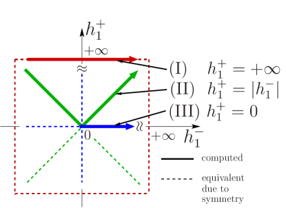
Figure 1: The parameter space spanned by the scaling variables $h_{1}^{+}$ and $h_{1}^{-}$ corresponding to the top and bottom surface fields $H_{1}^{+}$ and $H_{1}^{-}$, respectively (see Eq. (II)). We investigate the following paths: (I) $h_{1}^{+}=\infty$ (red line) corresponding to an infinitely strong surface field $H_{1}^{+}$, (II) $h_{1}^{+}=|h_{1}^{-}|$ (green line), (III) $h_{1}^{+}=0$ (blue line). Dashed lines of corresponding colors denote trajectories, which are equivalent due to the exchange symmetry $h_{1}^{+}\leftrightarrow h_{1}^{-}$. Since Eq. (2) does not contain a bulk field there is in addition the symmetry $(h_{1}^{+},h_{1}^{-})\leftrightarrow(-h_{1}^{+},-h_{1}^{-})$.

For a fixed width $L_{z}$ and a fixed aspect ratio $\rho=L_{z}/L_{x}=L_{z}/L_{y}$ of the slab, the thermodynamic state of the system is characterized by three parameters: $t,H_{1}^{-}$, and $H_{1}^{+}$. Based on finite-size scaling arguments, for the present system Fisher and Nakanishi fisher_nakanishi proposed the following convenient scaling variables associated with the surface fields:

$$h_{1}^{\pm}:=H_{1}^{\pm}L_{z}^{\Delta^{ord}_{1}/\nu} = (c\xi_{0}^{+})^{y}\left[L_{z}/(\ell_{1}^{\pm}/\xi_{0}^{+})\right]^{\Delta^{ord}_{1}/\nu}$$

$$\stackrel{{\scriptstyle D=3}}{{=}} (c\xi_{0}^{+})^{0.87}\left[L_{z}/(\ell_{1}^{\pm}/\xi_{0}^{+})\right]^{0.73};$$

$\ell^{-}_{1}$ and $\ell^{+}_{1}$ correspond to bottom and the top surface, respectively.

Here we study the following three trajectories (see Fig. 1):

• $h_{1}^{+}=\infty$,   an infinitely strong top surface field.

• $h_{1}^{+}=|h_{1}^{-}|$, finite symmetric and antisymmetric surface fields.

• $h_{1}^{+}=0$,      free boundary conditions at the top surface.

In the simulations, case (I) is realized by fixing all spins in the top layer $z=L_{z}$ at the value $+1$. For finite surface fields it is convenient to replace the surface field applied at the top (bottom) surface of the slab by having this surface layer being linked via modified bonds to spins located in an extra layer $z=0$ ( $z=L_{z}+1$) with the interaction $-H_{1}^{-}\sum_{x,y}s_{x,y,0}s_{x,y,1}$ ($-H_{1}^{+}\sum_{x,y}s_{x,y,L_{z}}s_{x,y,L_{z}+1}$); the spins in the extra layer $z=0$ ($z=L_{z}+1$) are fixed at the same value $+1$ for all $x,y$. In practice, a surface field, which is finite but strong enough to lead to a saturation of the data, can be used to mimic the action of an infinite surface field. For instance, for $|h_{1}^{+}|>100$ we do not observe any variation of our data as function of $h_{1}^{+}$.

By construction, for all three cases there is only one scaling variable associated with the two surface fields. In the following we use the notation $H_{1}\equiv H_{1}^{-}$ and $h_{1}\equiv h_{1}^{-}$. This fixes the top surface field $H_{1}^{+}$ in accordance with (I) - (III). The plane of parameters $(h_{1}^{-}=h_{1},h_{1}^{+})$ is shown in Fig. 1. We note that the cases (I) and (II) with symmetric fields coincide at the point $(\infty,\infty)$, the cases (II) with symmetric fields and (III) coincide for $(0,0)$, and finally for the cases (I) and (III) the point $(0,\infty)$ coincides with $(\infty,0)$.

We have computed the critical Casimir forces for a selection of parameters from sets corresponding to the cases (I), (II), and (III) which in Fig. 1 are denoted by solid lines. Points in the plane $(h_{1}^{-},h_{1}^{+})$ corresponding to the cases (I), (II), and (III) which are equivalent due to the exchange symmetry $h_{1}^{-}\leftrightarrow h_{1}^{+}$ are indicated by dashed lines. Due to the absence of a bulk field there is also the symmetry $(h_{1}^{+},h_{1}^{-})\leftrightarrow(-h_{1}^{+},-h_{1}^{-})$.

For large areas $A$, the total free energy $F(\beta,H_{1}^{+},H_{1}^{-},L_{z},A)$ of the film of thickness $L_{z}$ can be written as

$$\frac{F(\beta,H_{1}^{+},H_{1}^{-},L_{z},A)}{A}\equiv L_{z}f(\beta,H_{1}^{+},H_{1}^{-},L_{z})$$

$$= L_{z}f^{\mathrm{bulk}}(\beta)+\beta^{-1}f^{\mathrm{ex}}(\beta,H_{1}^{+},H_{1}^{-},L_{z}),$$

where $f^{\mathrm{bulk}}(\beta)$ is the bulk free energy density at a given temperature. The excess free energy $f^{\mathrm{ex}}$ per area contains two $L_{z}$-independent surface contributions in addition to the finite-size contribution $f^{\mathrm{ex}}(\beta,H_{1}^{+},H_{1}^{-},L_{z})-f^{\mathrm{ex}}(\beta,H_{1}^{+},H_{1}^{-},\infty)$ which vanishes for $L_{z}\to\infty$. The $L_{z}$-dependence of the latter gives rise to the critical Casimir force $f_{\mathrm{C}}$ per unit area $A$ and in units of $k_{\mathrm{B}}T\equiv\beta^{-1}$:

$$f_{\mathrm{C}}(\beta,H_{1}^{+},H_{1}^{-},L_{z})\equiv-\partial f^{\mathrm{ex}}(\beta,H_{1}^{+},H_{1}^{-},L_{z})/\partial L_{z},$$ (5)

with the bottom surface field $H_{1}^{-}=H_{1}$ and the upper surface field $H_{1}^{+}=\{\infty,|H_{1}^{-}|,0\}$, in accordance with (I), (II), and (III), respectively.

For a lattice (lattice quantities are denoted by a “hat” $\,\hat{}\,$), the derivative in Eq. (5) is replaced by a finite difference and $\hat{f}_{\mathrm{C}}(\beta,L)$ is given by

$$\hat{f}_{\mathrm{C}}(\beta,H_{1},L,A)\equiv-\frac{\beta\Delta\hat{F}(\beta,H_{1},L,A)}{A}+\beta\hat{f}^{\mathrm{bulk}}(\beta)\,,$$ (6)

with the free energy difference $\Delta\hat{F}(\beta,H_{1},L,A)=\hat{F}(\beta,H_{1},L+\frac{1}{2},A)-\hat{F}(\beta,H_{1},L-\frac{1}{2},A)$. In these three expressions the thickness $L=L_{z}-\frac{1}{2}$ is half-integer, so that the rhs is expressed via the free energy difference for slabs of integer thicknesses $L_{z}=L+\frac{1}{2}$ and $L_{z}-1=L-\frac{1}{2}$. Later on we shall denote by $L_{z}$ the thickness of the system for which we perform the computations and by the half-integer quantity $L=L_{z}-\frac{1}{2}$ the variable the critical Casimir force depends on.

From the general theory of finite-size scaling  fisher_nakanishi ; FSS and based on renormalization-group analyses krech:92 we expect that in the scaling limit the Casimir force takes the universal scaling form

$$f_{\mathrm{C}}(\beta,H_{1}^{+},H_{1}^{-},L)=L^{-d}\vartheta\left((L/\xi_{b})^{1/\nu}{\rm sign}(t),h_{1}^{+},h_{1}^{-}\right)$$ (7)

where the scaling function $\vartheta(\tau=(L/\xi_{0}^{+})^{1/\nu}t,h_{1}^{+},h_{1}^{-})$ depends on the spatial dimension $D$ and on the boundary conditions on the top and bottom surfaces. Here $\xi_{b}=\xi_{0}^{\pm}|t|^{-\nu}$ is the bulk correlation length which controls the spatial exponential decay of the two-point correlation function; $\xi_{0}^{\pm}$ are nonuniversal amplitudes above $(+)$ and below $(-)$ the bulk critical temperature $T_{c}$. In the whole range of temperatures, we plot the scaling functions using the value $\xi^{+}_{0}=0.501(2)$ RZW which is the amplitude of the second moment correlation length $\xi_{\mathrm{2^{nd}}}$; for the Ising model $\xi_{b}/\xi_{\mathrm{2^{nd}}}\simeq 1$ for $\beta<\beta_{c}$  PV .

Below we shall use the following notations: $\vartheta^{(I)}(\tau,h_{1})=\vartheta(\tau,h_{1}^{+}=\infty,h_{1}^{-})$, $\vartheta^{(II)}(\tau,h_{1})=\vartheta(\tau,h_{1}^{+}=|h_{1}^{-}|,h_{1}^{-})$, and $\vartheta^{(III)}(\tau,h_{1})=\vartheta(\tau,h_{1}^{+}=0,h_{1}^{-})$.

III Numerical method

We compute the free energy difference $\Delta\hat{F}(\beta,H_{1},L,A)$ by using the so-called coupling parameter approach (see, e.g., Refs. Mon and PRE ). This is a viable alternative to the method used in Ref. DK , in which a suitable lattice stress tensor has been introduced in such a way that its ensemble average renders $\Delta\hat{F}$. So far, this latter method can be implemented only for periodic BC.

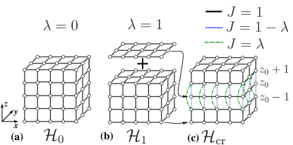
Figure 2: Bond arrangement for the computation of the free energy difference in Eq. (10) between systems of thickness $L_{z}$ (a) and $L_{z}-1$ (b) (see the main text). The crossover Hamiltonian ${\cal H}_{cr}$ (c) belongs to a system which interpolates between those described by the Hamiltonian ${\cal H}_{0}$ (a) for the system of thickness $L_{z}$ (for $\lambda=0$) and by the Hamiltonian ${\cal H}_{1}$ (b) for the system of thickness $L_{z}-1$ plus a 2D layer of area $A$ (for $\lambda=1$).

The coupling parameter approach is used in order to compute the difference $F_{1}-F_{0}$ between free energies $F_{i}=-\frac{1}{\beta}\ln\sum_{{\mathcal{C}}}\exp(-\beta{\cal H}_{i}),\;\;i=0,1$, of models characterized by two different energies as given by Hamiltonian ${\cal H}_{0}$ and ${\cal H}_{1}$. Such a calculation is successful if the configuration space ${\mathcal{C}}$ (i.e., the whole set of spins) is the same for both models. In order to implement this approach, one introduces an interpolating system with the crossover Hamiltonian

$${\cal H}_{\rm cr}(\lambda)=(1-\lambda){\cal H}_{0}+\lambda{\cal H}_{1}.$$ (8)

As a function of the coupling parameter $\lambda\in\left[0,1\right]$, ${\cal H}_{\rm cr}(\lambda)$ interpolates between ${\cal H}_{0}$ and ${\cal H}_{1}$ as $\lambda$ increases from 0 to 1. Accordingly the free energy $F_{\rm cr}(\lambda)=-\frac{1}{\beta}\ln\sum_{{\mathcal{C}}}\exp(-\beta{\cal H}_{\rm cr}(\lambda))$ of the crossover system interpolates between $F_{0}$ and $F_{1}$. The sum is taken over all spin configurations ${\mathcal{C}}$ of the model, which are the same for $F_{0},\;F_{1}$, and $F_{\rm cr}$. The difference $F_{1}-F_{0}$ can trivially be expressed as $F_{1}-F_{0}=\int_{0}^{1}F^{\prime}_{\rm cr}(\lambda){\rm d}\lambda$ where $F^{\prime}_{\rm cr}$ is the derivative of $F_{\rm cr}(\lambda)$ with respect to the coupling parameter:

$$\frac{{\rm d}F_{\rm cr}(\lambda)}{{\rm d}\lambda}=\frac{\sum_{\mathcal{C}}({\cal H}_{1}-{\cal H}_{0}){\rm e}^{-\beta{\cal H}_{\rm cr}(\lambda)}}{\sum_{\mathcal{C}}{\rm e}^{-\beta{\cal H}_{\rm cr}(\lambda)}}=\langle\Delta{\cal H}\rangle_{\rm cr}(\lambda)\,,$$ (9)

which takes the form of the canonical ensemble average $\langle\ldots\rangle_{\rm cr}(\lambda)$ of the energy difference $\Delta{\cal H}\equiv{\cal H}_{1}-{\cal H}_{0}$ with respect to the crossover Hamiltonian ${\cal H}_{\rm cr}$ for a given value of the coupling parameter $\lambda$. The energy difference $\langle\Delta{\cal H}\rangle_{\rm cr}(\lambda)$ can be computed efficiently via MC simulations of the lattice model characterized by the Hamiltonian ${\cal H}_{\rm cr}$. Finally, the difference of free energies is expressed as an integral over the mean energy difference (see, e.g., Ref. Mon ):

$$F_{1}-F_{0}=\int_{0}^{1}\langle\Delta{\cal H}\rangle_{\rm cr}(\lambda)\,{\rm d}\lambda.$$ (10)

According to Eq. (6) we are interested in the difference $\Delta\hat{F}(\beta,H_{1},L,A)$ between the free energies $\hat{F}(\beta,H_{1},L_{z},A)$ and $\hat{F}(\beta,H_{1},L_{z}-1,A)$ (we recall that $L=L_{z}-\frac{1}{2}$ ). In order to apply the method described above for the computation of $\Delta\hat{F}(\beta,H_{1},L,A)$ (which renders $\hat{f}_{\mathrm{C}}$ (see Eq. (6))) one identifies the model, the Hamiltonian ${\cal H}_{0}$, and the associated configuration space ${\mathcal{C}}$ with the corresponding quantities of the model we are interested in on the lattice $A\times L_{z}$ (see Fig. 2(a)) so that $\hat{F}_{0}(\beta,H_{1},L_{z},A)=\hat{F}(\beta,H_{1},L_{z},A)$. The final system ${\cal H}_{1}$ is identified with the slab of area $A$ and thickness $L_{z}-1$ plus a two-dimensional layer of size $A$: $\hat{F}_{1}(\beta,H_{1},L_{z},A)=\hat{F}(\beta,H_{1},L_{z}-1,A)+\hat{F}_{2D}(\beta,A)$ (see Fig. 2(b)). Here $\hat{F}_{2D}(\beta,A)$ is the free energy of the isolated 2D layer of area $A$. One has to include this 2D layer into the consideration in order to maintain the same number of spins in the configuration space ${\mathcal{C}}$ for the initial, intermediate, and final models. This layer can be extracted from the initial model at any position $z_{0}=1,2,\ldots,L_{z}$ along the $z$-direction. It decouples from the rest of the lattice upon passing from $\lambda=0$ to $\lambda=1$, i.e., from Fig. 2 (a) to (b) via (c). The corresponding crossover Hamiltonian ${\cal H}_{\rm cr}(\lambda)$ (but not the result of the integration in Eq.(10)) does depend on the position $z_{0}$ from where the $2D$ layer is extracted. In our simulations we use $z_{0}=L_{z}/2$ for even values of $L_{z}$ and $z_{0}=(L_{z}-1)/2$ for odd values of $L_{z}$. The explicit expression for the energy difference ${\cal H}_{1}-{\cal H}_{0}$ is

$$\Delta{\cal H} = -\sum_{x,y}\left(s_{x,y,z_{0}-1}s_{x,y,z_{0}+1}\right.$$

$$- \left.s_{x,y,z_{0}-1}s_{x,y,z_{0}}-s_{x,y,z_{0}}s_{x,y,z_{0}+1}\right)\;,$$

where the three indices $(x,y,z)$ identify a lattice site, the sum is taken over all lateral lattice site positions in the $xy$ plane, and with a coupling strength $J=1$ (indicated by solid bonds in Figs. 2 (a) and (b); $J$ is absorbed into $\beta$). The crossover Hamiltonian ${\cal H}_{\rm cr}(\lambda)={\cal H}_{0}+\lambda\Delta{\cal H}$ is characterized by the coupling constants depicted in Fig. 2(c). The free energy difference $\Delta\hat{F}$ (see Eqs. (6) and (10)) can be expressed as

$$\Delta\hat{F}(\beta,H_{1},L,A)=-\int_{0}^{1}\langle\Delta{\cal H}\rangle_{\rm cr}(\lambda){\rm d}\lambda+F_{2D}(\beta,A)$$ (12)

where the integral is taken for fixed values of $\beta$ and $H_{1}$. Note that although $\Delta{\cal H}$ is independent of $H_{1}$, the dependence of $\Delta\hat{F}$ on $H_{1}$ enters via the statistical weight $\sim\exp(-\beta{\cal H}_{\rm cr})$. The free energy $F_{2D}(\beta,A)$ of the 2D layer can be computed from the analytical expressions given in Ref. Kauf .

Once $\Delta\hat{F}(\beta,H_{1},L,A)$ has been computed, one has still to subtract $f^{\mathrm{bulk}}(\beta)$ from it (see Eq. (6)) in order to obtain the Casimir force for a slab of assigned thickness $L=L_{z}-1/2$. We determine the bulk free energy by using the temperature integration method hucht ; hasen1 ; hasen2 applied to a cubical system of size $L_{\rm cube}$ with periodic boundary conditions. For such a system the free energy per site (in units of $k_{B}T$) can be written as

$$\beta\hat{f}(\beta,L_{\rm cube})=-\ln(2)+\frac{1}{L_{\rm cube}^{3}}\int\limits_{0}^{\beta}\langle E(\beta^{\prime},L_{\rm cube})\rangle{\rm d}\beta^{\prime},$$ (13)

where $\langle E(\beta^{\prime},L_{\rm cube})\rangle$ is the averaged internal energy of the system at the inverse temperature $\beta^{\prime}$ and for the size $L_{\rm cube}$; $-\ln(2)$ is the free energy in units of $k_{B}T$ and per site at $\beta=0$. For a cube, in the limit $L_{cube}\to\infty$ the finite-size dependence of the free energy density for a cube is predicted FSS to scale with $L_{cube}$ as $\beta\hat{f}(\beta,L_{\rm cube})-\beta f^{\rm bulk}(\beta)\propto L^{-3}_{\rm cube}$. Therefore the bulk free energy per spin follows as the limit $\beta f^{\rm bulk}(\beta)=\lim\limits_{L_{\rm cube}\to\infty}\left[\beta\hat{f}(\beta,L_{\rm cube})\right]$. At the critical point one has

$$\beta_{c}\hat{f}(\beta_{c},L_{\rm cube})\simeq\beta_{c}f^{\rm bulk}(\beta_{c})+U_{0}L^{-3}_{\rm cube},$$ (14)

with the universal finite-size scaling amplitude $U_{0}=-0.657(3)$ (see Ref. Mon ).

In order to determine the universal scaling function of the critical Casimir force we perform the following steps (details are given below). For each temperature we compute the averaged internal energy $\langle E(\beta,L_{\rm cube})\rangle$ for a cube with periodic boundary conditions by using a histogram reweighting MC method. Then we carry out a numerical integration in order to obtain an estimate for the bulk free energy $\beta f^{\rm bulk}(\beta)$ in accordance with Eqs. (13) and (14). For the slab geometry $A\times L_{z}$, at the inverse temperature $\beta$, and for a fixed boundary field $H_{1}$, we compute the ensemble averages $\langle\Delta{\cal H}\rangle_{cr}(\lambda)$ via MC simulations for $N_{\lambda}=21$ different values of $\lambda_{k}=\frac{k}{N_{\lambda}-1},k=0,\ldots,N_{\lambda-1}$. Based on these $N_{\lambda}$ values we carry out the numerical integration in Eq. (12) and use an analytical expression for $F_{2D}(\beta,A)$ in order to obtain $\Delta\hat{F}(\beta,H_{1},L,A)$. Combining the results for the bulk free energy density $\beta f^{\rm bulk}(\beta)$ and for the free energy difference and by using Eq. (6) we obtain a numerical estimate for the critical Casimir force $\hat{f}_{\mathrm{C}}(\beta,H_{1},L,A)$. In order to obtain the corresponding scaling function $\hat{\vartheta}$ we perform computations for various values of $L$, $A$, the inverse temperature $\beta$, and boundary fields $H_{1}$. The scaling function $\hat{\vartheta}$ in Eq. (7) is retrieved from the numerical data for $\hat{f}_{\mathrm{C}}$ by taking into account finite-size corrections as described in the following section.

For determining the bulk free energy density the histogram reweighting method has been used as follows  FS ; LB . The computation of the energy distribution $P(E,\beta_{i})$ has been performed for a choice of 256 points $\beta_{i}\in[0,0.3]$ for a cubic system of size $L_{\rm cube}=128$. For the numerical simulation we have employed the hybrid MC method, which is a suitable mixture of Wolff and Metropolis algorithms  LB . For thermalization $4\times 10^{5}$ hybrid MC steps have been used. The averaging has been performed over $10^{6}$ hybrid MC steps which have been split into 10 series for the evaluation of statistical errors. Therefore, for every value $\beta_{i}$ actually ten histograms (each consisting of $10^{5}$ MC steps) have been computed. According to the histogram reweighting method one can obtain an estimate for $\langle E\rangle$ at an inverse temperature $\beta^{\prime}$ based on the histogram $P(E,\beta_{i})$ for the inverse temperature $\beta_{i}$  FS ; LB :

$$\langle E\rangle_{\beta_{i}}(\beta^{\prime})=\frac{\sum\limits_{E}EP(E,\beta_{i})e^{-E(\beta^{\prime}-\beta_{i})}}{\sum\limits_{E}P(E,\beta_{i})e^{-E(\beta^{\prime}-\beta_{i})}}.$$ (15)

For every $\beta^{\prime}\in[\beta_{i},\beta_{i+1}]$ we define the interpolated internal energy

$$\langle E\rangle(\beta^{\prime})=\frac{\beta_{i+1}-\beta^{\prime}}{\beta_{i+1}-\beta_{i}}\langle E\rangle_{\beta_{i}}(\beta^{\prime})+\frac{\beta^{\prime}-\beta_{i}}{\beta_{i+1}-\beta_{i}}\langle E\rangle_{\beta_{i+1}}(\beta^{\prime}).$$ (16)

We have checked that for the same inverse temperature $\beta^{\prime}$ the difference between the estimates $\langle E\rangle_{\beta_{i}}(\beta^{\prime})$ and $\langle E\rangle_{\beta_{i+1}}(\beta^{\prime})$, which use histograms for two neighboring points $\beta_{i}$ and $\beta_{i+1}$, is substantially less than the statistical inaccuracy of our simulation data. The statistical inaccuracy has been determined canonically over 10 series of histograms. In the next step, in accordance with Eq. (13) we obtain the free energy $\beta\hat{f}(\beta,L_{cube})$ by integrating numerically the interpolated internal energy. For the intergration we employ the trapezoidal rule with a large $(>10^{5})$ number of points, so that the inaccuracy of the numerical integration is less then $10^{-9}$. We estimate that at the bulk critical temperature $\beta_{c}$ the statistical error $\Delta\beta_{c}\hat{f}(\beta_{c},L_{cube})$ for the free energy determined from 10 series is about $4\times 10^{-7}$. In the following, we neglect the finite-size correction of the bulk free energy and take $\beta f^{\rm bulk}(\beta)\simeq\beta\hat{f}(\beta,L_{\rm cube}=128)$ (compare Eq. (14)). This is justified, because for the maximal value $L=19.5$ used in our simulation the finite-size correction to $\vartheta$ due to the finite system size $L_{\rm cube}=128$, i.e., $0.657(L/L_{cube})^{3}\simeq 0.0023$, is of the same order as the statistical error stemming from the contributon $L^{3}\Delta\beta_{c}\hat{f}(\beta_{c},L_{cube})$, i.e., $(19.5)^{3}\times 4\times 10^{-7}\simeq 0.00297$ (see Eqs. (6) and (7)).

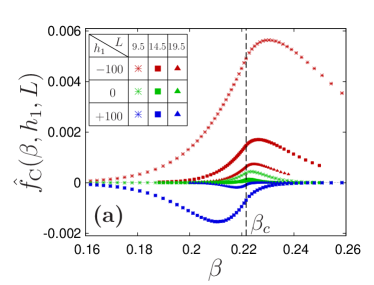
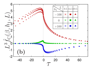
Figure 3: MC data for case (I): (a) Casimir force ${\hat{f}}_{\mathrm{C}}$ as a function of the inverse temperature $\beta$; $\beta_{c}=0.2216544(3)$ (b) rescaled Casimir force $L^{3}{\hat{f}}_{\mathrm{C}}$ as a function of the scaling variable $\tau=(L/\xi_{0}^{+})^{1/\nu}(T-T_{c})/T_{c}=(L/\xi_{0}^{+})^{1/\nu}t$. The data correspond to $h_{1}=-100,0,100$ and $L=9.5,14.5,19.5$. In (a) and (b) the data for $(h_{1},L)=(100,9.5)$ and $(100,14.5)$ as well as $(0,14.5)$ and $(0,19.5)$ can be barely distinguished.

For the computation of the free energy $\Delta\hat{F}(\beta,H_{1},L,A)$ in Eq. (6) we use slabs of thicknesses $L_{z}=10,15,20$, so that $L=9.5,14.5,19.5$, with an aspect ratio equal to 6: $L_{x}=L_{y}=6L_{z}$, $A=36L_{z}^{2}$. In order to compute the average $\langle\Delta{\cal H}\rangle_{\rm cr}(\lambda)$ we again use the hybrid MC method with a mixture of Wolff and Metropolis algorithms. Each hybrid MC step consists of a flip of a Wolff cluster according to the Wolff algorithm, followed first by $3A$ attempts to flip an arbitrary spin and then by $3A$ attempts to flip a spin $s_{x,y,z}$ with $z\in\{z_{0}-1,z_{0},z_{0}+1\}$. These attempts are accepted according to the Metropolis rate LB . We use $2.5\times 10^{5}$ MC steps for thermalization. For the computation of the thermal average we use $5\times 10^{5}$ MC steps split into 10 series. For each series, using Simpson’s rule we perform a numerical integration over $N_{\lambda}=21$ points for fixed values of the inverse temperature $\beta$, the surface field $H_{1}$, and the width $L$ of the slab. Having computed the free energy difference $\Delta\hat{F}(\beta,H_{1},L,A)$, for each series we finally combine the results for the bulk free energy $\beta\hat{f}^{\rm bulk}(\beta)$ with the corresponding ones for the free energy difference $\Delta\hat{F}(\beta,H_{1},L,A)$ and determine the numerical inaccuracy.

In Fig. 3(a) we plot the Casimir force ${\hat{f}}_{{\mathcal{C}}}$ as a function of $\beta$ for the three values $h_{1}=-100,0,100$ of the bottom surface scaling field. In Fig. 3(b) we plot the rescaled values of the Casimir force $L^{3}{\hat{f}}_{C}$ as a function of the temperature scaling variable $\tau=(L/\xi_{0}^{+})^{1/\nu}(T-T_{c})/T_{c}=(L/\xi_{0}^{+})^{1/\nu}t$ for case (I). The visible absence of the expected data collapse is due to finite size corrections to scaling, which will be discussed in the following section.

IV Finite size corrections to scaling

Finite-size scaling is known to be valid asymptotically for finite but large lattices and small values of $t$, i.e., for a large bulk correlation length $\xi_{b}$; here large means relative to the lattice constant  FSS . Outside the asymptotic regime corrections to the leading (universal) scaling behavior become relevant. These non-universal corrections affect both the scaling variables and the scaling functions and depend on the details of the model as well as on the geometry and the boundary conditions privman ; luck . Renormalization-group analyses reveal that there is a whole variety of sources for corrections to scaling which arise from bulk, surface, and finite-size effects FSS .

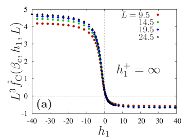
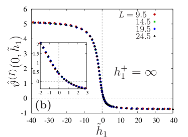
Figure 4: Results at the critical point $\beta=\beta_{c}$ for case (I) (see Fig. 1) as a function of boundary fields: (a) Casimir force multiplied by $L^{3}$ as a function of the scaling variable $h_{1}=H_{1}L^{\Delta^{ord}_{1}/\nu}$ without finite size corrections; (b) Casimir force scaling function $\hat{\vartheta}^{(I)}(\tilde{\tau}=0,\tilde{h}_{1})$ with taking corrections $L+\delta$ into account as a function of the corrected scaling variable $\tilde{h}_{1}=H_{1}(L+\delta)^{\Delta_{1}^{ord}/\nu}$; in units of the lattice spacing $\delta=0.65$ at the bulk critical point $\beta_{c}$. For $\tilde{h}_{1}=0$ one finds the fixed-point $(O,+)$.

For the finite and rather limited sizes of the lattices which we investigate in our MC simulations, it is necessary to take corrections to scaling into account in order to obtain data collapse and thus allowing us to infer the leading universal scaling function  hucht ; EPL ; PRE .

In the present study, the following quantities are expected to acquire corrections to scaling:

• the amplitude of the scaling function $\vartheta=L^{3}f_{{\mathcal{C}}}$

• the surface field scaling variable $h_{1}$

• the temperature scaling variable $\tau=t\left(L/\xi_{0}^{+}\right)^{1/\nu}$.

In our previous MC simulations aimed at obtaining critical Casimir forces for Ising films with a variety of universal boundary conditions, such as $(+,+),(+,-)$, or $(O,O)$ BC  EPL ; PRE , corrections to scaling were taken into account by using various ansätze. The choice for a particular form of corrections to scaling was guided by achieving the best data collapse or the best fits used in our computations. For example, for the amplitude of the scaling function we adopted the expression $\hat{f}_{\mathrm{C}}=L^{-3}\frac{(1+g_{1}L^{-1})}{(1+g_{2}L^{-1})}\hat{\vartheta}$. Various variants for this form of corrections to scaling were considered; we used $(g_{1}\neq 0,g_{2}),(g_{1},g_{2}\neq 0)$, or $(g_{1}\neq 0,g_{2}\neq 0)$. They all lead to a satisfactory data collapse, but the inferred amplitude of the scaling function of the critical Casimir force depends sensitively on the particular ansatz.

In Refs. hasen1 ; hasen2 still another type of finite-size correction is employed. It amounts to introducing an effective width $L+\delta$ of the slab so that, e.g., the amplitude of the scaling function of the critical Casimir force scales as $\hat{f}_{\mathrm{C}}=(L+\delta)^{-3}\hat{\vartheta}$. Using this type of finite-size correction may be justified as follows. As mentioned in Sec. I surfaces subjected to the action of a surface field asymptotically belong to the surface universality class of the normal transition which corresponds to $(+)$ or $(-)$ fixed-point boundary conditions in the sense of renormalization-group theory binder:83:0 ; diehl:86:0 . (The $(+)$ and $(-)$ boundary conditions are realized as the limits of the scaling field $h_{1}^{(i)}\rightarrow+\infty$ and $-\infty$, respectively.) For such boundary conditions, on the coarsed-grained scale the order parameter varies as $|\phi(z\to 0)|\propto z^{-\beta/\nu}$ for small normal distances from the surface (but still large on molecular scales) diehl:97 ; leibler . Within a certain range of small $z$ values such a divergent behavior is expected to hold also for a finite but sufficiently strong surface field. In Ising lattice models with boundary conditions corresponding to $(+)$ or $(-)$ fixed-point BCs, the order parameter does not diverge at the surface but saturates there at the value $+1$ or $-1$. Changing the width of the slab from $L$ to $L+\delta$ with a nonuniversal length $\delta=z_{\rm ex}^{(1)}+z_{\rm ex}^{(2)}$ such that the order parameter profile behaves as $|\phi(z\rightarrow 0)|\sim(z+z_{\rm ex}^{(i)})^{-\beta/\nu}$ binder:83:0 ; SDL-94 upon approaching the wall $i$, turns out to be an effective means to take into account corrections to the leading critical behavior SDL-94 ; $z_{\rm ex}^{(i)}$ plays the role of an extrapolation length binder:83:0 ; diehl:86:0 . Similarly, the effects of a physical wall with a finite surface field (which implies $\ell_{1}^{(i)}\neq 0$ ( see Eq. (1))) on the order parameter are equivalent to those of a fictitious wall with strong surface fields (which means $\ell_{1}^{(i)}=0$) displaced by a distance $-z_{\rm ex}^{(i)}$ from the physical wall. One can determine the length $\delta$ by analyzing the spatial variation of the order parameter profile, as it was done for the Blume-Capel model in Ref. hasen2 . Here, we assume that the equivalence described above carries over to critical Casimir forces such that we can determine the effective width $L+\delta$ of the slab by demanding the best data collapse. We apply this method also in the crossover regime, i.e., for sufficiently weak surface fields for which upon approaching the critical point one effectively observes a crossover to the boundary condition corresponding to the ordinary transition $(O)$ fixed point. As discussed in the introduction, the order parameter profiles in a film with weak surface fields deviate strongly from the fixed-point universal behavior. Accordingly, we expect that within this range of surface fields the aforementioned type of correction does not satisfactorily capture the actually corrections to scaling.

In Fig. 4(a) we plot the rescaled critical Casimir force $L^{3}{\hat{f}}_{{\mathcal{C}}}$ for case (I). It is evaluated at the critical point $\beta_{c}$ and presented as a function of $h_{1}$ without finite-size corrections taken into account. Apparently the data for the rescaled force do not coincide for various values of $L=9.5,14.5,19.5,24.5$. In order to obtain the expected data collapse we apply the following finite-size corrections (here and in the following we denote scaling variables with finite size corrections by a tilde: $\tilde{\tau}$, $\tilde{h}_{1}$):

$$\hat{f}_{{\mathcal{C}}}(\beta,H_{1},L,A)=(L+\delta)^{-3}\hat{\vartheta}(\tilde{\tau},\tilde{h}_{1})$$ (17)

with

$$\tilde{\tau}\equiv\tau\left[(L+\delta)/\xi_{0}^{+}\right]^{1/\nu}\left[1+g_{\omega}(L+\delta)^{-\omega}\right]$$ (18)

and (see Eq. (II))

$$\tilde{h}_{1}=H_{1}(L+\delta)^{\Delta^{ord}_{1}/\nu},$$ (19)

where $\omega=0.84(4)$ is the leading bulk correction-to-scaling exponent PV ; the length $\delta$ and the coefficient $g_{\omega}$ remain to be determined.

The value of the length $\delta$ is obtained from the data for the critical Casimir force at the critical point (these data are presented in Fig. 4(a)). By using Eqs. (17) and (19) and by implementing the fitting procedure within the interval $\tilde{h}_{1}\in[-15,15]$ with $\delta$ being the only fit parameter, we obtain the value $\delta=0.65$ which minimizes deviations between data for different values of $L$. Including error bars we find $\delta=0.65(2)$ for various intervals of $h_{1}$ or $\delta=0.60(5)$ for different sets of $L$. The final result for the scaling function $\hat{\vartheta}(0,\tilde{h}_{1})$ with corrections to scaling corresponding to $\delta=0.65$ is shown in Fig. 4(b). For large absolute values of $\tilde{h}_{1}$ we reproduce the data from Refs. EPL ; PRE for the critical point with $(-,+)$ and $(+,+)$ BCs. For small values of $|\tilde{h}_{1}|$ we observe the crossover between these two regimes.

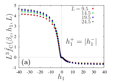
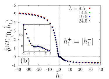
Figure 5: Same as Fig. 4 for the case (II) (see Fig. 1). For $\tilde{h}_{1}=0$ one finds the fixed point $(O,O)$.

The procedure which we used in order to obtain the best fit for the value of the length $\delta$ is described in detail in the appendix of Ref. PRE . One of the difficulties in finding the optimal data collapse is that the fitting function itself, i.e., the scaling function of the critical Casimir force, is not known. For the initial guess for the value of the length $\delta$ we infer the scaling function from the corresponding data for ${\hat{f}}_{{\mathcal{C}}}$, one function $\hat{\vartheta}_{k}$ for each value $L_{k}$ $(k=1,\cdots,N)$ used (see Eqs. (17), (18), and (19)). We define an expected scaling function as the average of the various $\hat{\vartheta}_{k}$: $\hat{\vartheta}_{expected}=(1/N)\sum_{k=1}^{N}\hat{\vartheta}_{k}$. Finally, for every $L_{k}$ and for a given value of $\delta$ we compute the sum of squares $\chi^{2}(\delta)$ of the deviation of the aforementioned scaling functions from the expected scaling function. Finally, we determine as the value of $\delta$ the one which minimizes $\chi^{2}$. That value provides the best data collapse of the data for different $L$.

Applying the same procedure for case (II) and case (III) we obtain the values $\delta=0.6$ and $\delta=1.4$, respectively. However, in order to be consistent (as mentioned earlier, for some values of the surface field different cases coincide) we use the common value $\delta=0.65$ for all cases. In Figs. 5 and 6 we present our results without (a) and with (b) finite-size corrections for case (II) and case (III), respectively.

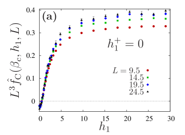
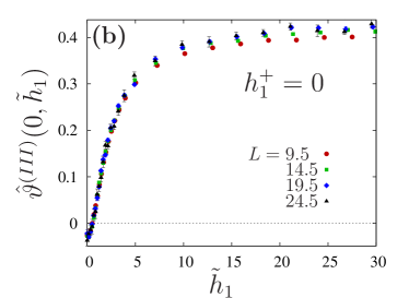
Figure 6: Same as Fig. 4 for the case (III) (see Fig. 1). For $\tilde{h}_{1}=0$ one finds the fixed point $(O,O)$.

Knowing the finite-size corrections of the surface field scaling variable we can carry out numerical simulations for various values of $\tilde{h}_{1}$; for each value of $\tilde{h}_{1}$ we can extract information about the coefficient $g_{\omega}$ using the same procedure as for the determination of the length $\delta$.

V Results

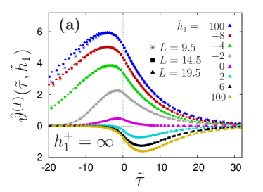
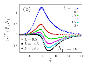
Figure 7: The scaling function $\hat{\vartheta}^{(I)}$ of the critical Casimir force for case (I), i.e., $h_{1}^{+}=\infty$ as a function of the temperature scaling variable $\tilde{\tau}$ (see Eq. (18)) for various bottom boundary fields corresponding to certain values of the surface field scaling variable $\tilde{h}_{1}\equiv\tilde{h}_{1}^{-}$ (see Eq. (19)): (a) large amplitudes of the surface field (from top to bottom): $\tilde{h}_{1}=-100,-8,-4,-2,0,2,6,100$; (b) small amplitudes of the surface field for which a crossover from repulsive to attractive forces as function of $\tilde{\tau}$ is observed (from top to bottom): $\tilde{h}_{1}=-1,0,0.5,1,1.5,2$. For each color $\bigstar$ corresponds to $L=9.5$, $\blacksquare$ to $L=14.5$, and $\blacktriangle$ to $L=19.5$.

Here we present the critical Casimir force scaling function determined for various values of $\tilde{h}_{1}$ as a function of $\tilde{\tau}$. The set of values used for $\tilde{h}_{1}$ is given in Tables 1, 2, and 3. For each of the three values $L=9.5,14.5,19.5$ of the slab thickness we infer the values of the surface fields $H_{1}$ which correspond to the pair $(\tilde{h}_{1},L)$ according to Eq. (19) with $\delta=0.65$. Next, for each pair $(\tilde{h}_{1},L)$ the critical Casimir force $\hat{f}_{{\mathcal{C}}}(\beta,H_{1},L)$ has been computed for various inverse temperatures $\beta$. Finally, for each value of $\tilde{h}_{1}$ we apply the fitting procedure described above in order to determine $g_{\omega}$ by using Eq. (18). Our results for $g_{\omega}$ are given in Tables 1, 2, and 3 for the cases (I), (II), and (III), respectively.

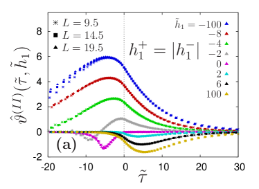
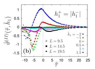
Figure 8: Same as Fig. 7 for case (II) (see Fig. 1). In (b) for small amplitudes of the surface field [from top to bottom: $\tilde{h}_{1}\equiv\tilde{h}^{-}_{1}=-2,-1,0,0.5,1,1.5$] there occurs a crossover from attractive to repulsive forces upon increasing $\tilde{\tau}$.

Table 1: Values of $\tilde{h}_{1}$ with the corresponding values of $g_{\omega}$ as obtained from the fitting procedure for case (I), i.e., $h_{1}^{+}=\infty$.

$\tilde{h}_{1}$	-100	-8	-4	-2	-1	0
$g_{\omega}$	-0.56(2)	-0.05(2)	-1.19(2)	1.04(2)	1.60(4)	2.3(2)
$\tilde{h}_{1}$	0.5	1	1.5	2	6	100
$g_{\omega}$	0.68(12)	0.72(15)	-0.05(5)	-0.145(3)	-0.47(2)	-0.94(2)

Table 2: Same as Table 1 for case (II), i.e., $h_{1}^{+}=|h_{1}|$.

$\tilde{h}_{1}$	-100	-8	-4	-2	-1	0
$g_{\omega}$	-0.58(2)	-0.14(2)	-0.25(2)	0.18(2)	0.10(3)	0.70(3)
$\tilde{h}_{1}$	0.5	1	1.5	2	6	100
$g_{\omega}$	2.05(10)	0.51(10)	0.97(13)	1.30(5)	-0.06(2)	-0.95(2)

Table 3: Same as Table 1 for case (III), i.e., $h_{1}^{+}=0$.

$\tilde{h}_{1}$	100	6	2	1	0.5	0
$g_{\omega}$	2.8(1)	1.6(1)	-0.12(5)	1.51(5)	1.87(4)	1.30(3)

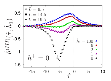
Figure 9: Same as Fig. 7 for case (III) ($\tilde{h}_{1}\equiv\tilde{h}_{1}^{-}$ see Fig. 1).

For a selection of values of the surface field scaling variable $\tilde{h}_{1}$ in Fig. 7(a) we present our results for the critical Casimir force scaling function $\hat{\vartheta}^{(I)}(\tilde{\tau},\tilde{h}_{1})$ corresponding to case (I). We find that de facto for $\tilde{h}_{1}=\pm 100$ the scaling limit of infinitely strong surface fields has been reached and the scaling function of the critical Casimir force corresponds to the fixed-point BCs $(+,\pm)$. In Fig. 7(b) we present our results for small values of $|\tilde{h}_{1}|$, $\tilde{h}_{1}\in[-1,2]$, for which we observe a transition from a repulsive to an attractive force upon increasing the temperature scaling field $\tilde{\tau}$. In these instances in which a change in sign is observed in Fig. 7(b), the length scales associated with the surface fields are $\ell_{1}^{+}=0$ (see Eq. (1) for $H_{1}^{+}=\infty$) on the top and $|\ell_{1}^{-}/\xi_{0}^{+}|=0.44L_{z}$ (see Eqs. (1) and (II) for $h_{1}=1$ and $c=0.5/\xi_{0}^{+}$) and $|\ell_{1}^{-}/\xi_{0}^{+}|\simeq 1.13L_{z}$ (see Eqs. (1) and (II) for $h_{1}=0.5$ and $c=0.5/\xi_{0}^{+}$) on the bottom. (In $D=3$, $c=1/a$ if the coupling constant in the surface row is unchanged relative to the one in the bulk binder:83:0 ; diehl:86:0 ; with $\xi_{0}^{+}\simeq 0.501$ this implies $c\xi_{0}^{+}\simeq 0.501$.)

In Fig. 8(a) we show data for the critical Casimir force scaling function $\hat{\vartheta}^{(II)}(\tilde{\tau},\tilde{h}_{1})$ corresponding to case (II). For $\tilde{h}_{1}=100$ and $\tilde{h}_{1}=-100$ we recover the scaling limit corresponding to $(++)$ and $(+-)$ fixed-point BCs, respectively. We note that the change in sign of the critical Casimir force upon varying the temperature occurs only for opposing surface fields. As before this change of sign is observed for weak surface fields for which $|\ell_{1}^{-}/\xi_{0}^{+}|\approx L_{z}$, i.e., for $\tilde{h}_{1}=-2,-1$.

Finally, in Fig. 9 the data for case (III) are presented. This case contains in particular two fixed-point BCs: for the value $\tilde{h}_{1}=100$ we observe a universal behavior of the scaling function of the critical Casimir force corresponding to $(O,+)$ fixed-point BCs, whereas for $\tilde{h}_{1}=0$ we find the $(O,O)$ fixed-point universal behavior of $\hat{\vartheta}(\tilde{\tau},\tilde{h}_{1})$. As in the other cases, the crossover from attraction to repulsion can be achieved by increasing the temperature scaling variable $\tilde{\tau}$, provided that the surface fields are sufficiently weak so that $|\ell_{1}^{-}/\xi_{0}^{+}|\approx L_{z}$, i.e., for $\tilde{h}_{1}=2$ and 1.

VI Summary and Conclusions

For variable surface fields we have determined via MC simulations the universal scaling functions $\hat{\vartheta}$ of critical Casimir forces for $3D$ Ising slabs describing the crossover from the ordinary to the normal surface universality class (Figs. 7, 8, and 9). This amounts to investigate the scaling functions $\vartheta(\tau,h_{1}^{+},h_{1}^{-})$ (see Eq. (7)) for finite values of the surface fields. We have computed the lattice scaling functions $\hat{\vartheta}(\tilde{\tau},\tilde{h}_{1})$ along three different paths in the parameter space $(h_{1}^{+},h_{1}^{-})$ (see Fig. 1): $\hat{\vartheta}^{(I)}(\tilde{\tau},\tilde{h}_{1})$ corresponding to $h_{1}^{+}=\infty$, $\hat{\vartheta}^{(II)}(\tilde{\tau},\tilde{h}_{1})$ corresponding to $h_{1}^{+}=|h_{1}^{-}|$, and $\hat{\vartheta}^{(II|)}(\tilde{\tau},\tilde{h}_{1})$ corresponding to $h_{1}^{+}=0$. Due to the fact that on the lattice the derivative in Eq. (5) is replaced by a finite difference, the scaling function $\hat{\vartheta}$ as function of the corrected scaling variables $(\tilde{\tau},\tilde{h}_{1})$ estimates the leading behavior of $\vartheta$ as function of $(\tau,h_{1}^{+},h_{1}^{-})$; alternative definitions of the lattice derivative give rise to distinct corrections for both the scaling function and the scaling variables. We have focused on cases in which upon variation of the temperature a crossover from attractive to repulsive critical Casimir force is observed. Such a behavior is particularly interesting in view of potential application, e.g., for colloidal suspensions. We have found that a change of sign of the critical Casimir force as a result of a minute change in temperature occurs only in systems with strongly asymmetrical surfaces, i.e., in cases in which the two surface fields differ significantly in magnitude. For this phenomenon to occur at least one of the surface fields has to be weak enough such that the length scale $\ell_{1}$ associated with the surface field $H_{1}$ (Eq. (1)) is comparable with the width $L$ of the slab (see Figs. 7(b) and 9 corresponding to fixed $h_{1}^{+}=\infty$ and $h_{1}^{+}=0$, respectively, and a variable second surface scaling field $h_{1}^{-}$). We note that for such large values of $\ell_{1}$ the order parameter profiles near a single wall differ significantly from the ones corresponding to strong surface fields which belong to the surface universality class of the normal transition. If both surface fields are weak and have the same magnitude they must have opposite signs in order to produce a change of sign of the critical Casimir force (see Fig. 8(b)). The change from attraction to repulsion (i.e., a zero of $\hat{\vartheta}$) can occur either below the bulk critical temperature, as for the cases in which one of the surfaces is subjected to the $(O)$ fixed-point BC or for weak opposing surface fields (see Figs. 9 and 8, respectively), or above $T_{c}$, as for the $(+)$ fixed-point BC (see Fig. 7(b)). In all cases the change of sign takes place rather close to the critical point.

Corrections to scaling have had to be taken into account in order to obtain data collapse which allowed us to infer the universal scaling functions (see Fig. 3). The introduction of an effective width $L+\delta$ of the slab turned out to be a very useful way of implementing corrections to scaling, provided the surface fields are not too weak. The value of the length $\delta$ has been obtained from the data for the critical Casimir force at the critical point (see Figs. 4 and 6 corresponding to fixed values $h_{1}^{+}=\infty$ and $h_{1}^{+}=0$ for the top surface, respectively, and a variable surface scaling field $h_{1}^{-}$ for the bottom surface, and Fig. 5 corresponding to the surface fields for the two surfaces to be of the same magnitude; compare Fig. 1).

The present results close an important gap in the knowledge of the Casimir scaling function for the $3D$ Ising universality class. The theoretical results for variable surface fields have been available in $D=2$ (from exact calculations in Ising strips abraham_maciolek ) and in $D=4$ (from a field-theoretic approach MMD ). The MC simulation results in Ref. hasen2 have been obtained for the $3D$ Blume-Capel model which is an extension of the Ising model studied here. They provide critical Casimir forces as function of $\beta_{c}-\beta$ for certain values of the surface fields, which in the parameter space shown in Fig. 1 correspond to path $(I)$ with $h_{1}^{-}\geq 0$. Because the choice of the surface fields for the presented data is different from ours, we cannot make a direct quantitative comparison (except for the case of ($h_{1}^{+}=\infty,h_{1}^{-}=0$) for which the data agree). However, there is a qualitative agreement with our findings; for certain choices of the surface fields the critical Casimir force changes sign as function of temperature. This agreement provides further evidence for the universal character of critical Casimir forces.

Our data for the critical Casimir scaling function have the crucial advantage over the results in $D=2$ and 4 that they can be directly compared with possible experimental data. Interestingly, in all spatial dimensions studied the crossover behavior of the scaling function of the critical Casimir force as a function of the temperature scaling variable is qualitatively the same. The robustness of this observation indicates that an experimental observation of the change of sign of the critical Casimir force with temperature is possible, provided that the chemical properties of the confining surfaces are carefuly chosen.

References

- (1) M. E. Fisher and P. G. de Gennes, C. R. Acad. Sci. Paris Ser. B 287, 207 (1978).
- (2) M. Krech, Casimir Effect in Critical Systems (World Scientific, Singapore, 1994); J. Phys.: Condens. Matter 11, R391 (1999).
- (3) J. G. Brankov, D. M. Dantchev, and N. S. Tonchev, The Theory of Critical Phenomena in Finite-Size Systems - Scaling and Quantum Effects (World Scientific, Singapore, 2000).
- (4) for a recent review see A. Gambassi, J. Phys.: Conf. Ser. 161, 012037 (2009).
- (5) U. Nellen, J. Dietrich, L. Helden, S. Chodankar, K. Nygård, J. F. van der Veen, and C. Bechinger, Soft Matter 7, 5360 (2011).
- (6) R. Garcia and M. H. W. Chan, Phys. Rev. Lett. 83, 1187 (1999); A. Ganshin, S. Scheidemantel, R. Garcia, and M. H. W. Chan, Phys. Rev. Lett. 97, 075301 (2006).
- (7) R. Garcia and M. H. W. Chan, Phys. Rev. Lett. 88, 086101 (2002).
- (8) M. Fukuto, Y. F. Yano, and P. S. Pershan, Phys. Rev. Lett. 94, 135702 (2005).
- (9) S. Rafaï, D. Bonn, and J. Meunier, Physica A 386, 31 (2007).
- (10) O. Vasilyev, A. Gambassi, A. Maciołek, and S. Dietrich, EPL 80, 60009 (2007).
- (11) O. Vasilyev, A. Gambassi, A. Maciołek, and S. Dietrich, Phys. Rev. E 79, 041142 (2009).
- (12) A. Hucht, Phys. Rev. Lett. 99, 185301 (2007).
- (13) R. Zandi, J. Rudnick, and M. Kardar, Phys. Rev. Lett. 93, 155302 (2004); R. Zandi, A. Shackell, J. Rudnick, M. Kardar, and L. P. Chayes, Phys. Rev. E 76, 030601(R) (2007).
- (14) A. Maciołek, A. Gambassi, and S. Dietrich, Phys. Rev. E 76, 031124 (2007).
- (15) A. Maciołek, and S. Dietrich, Europhys. Lett. 74, 22 (2006).
- (16) M. Krech, Phys. Rev. E 56, 1642 (1997).
- (17) Z. Borjan and P. J. Upton, Phys. Rev. Lett. 101, 125702 (2008).
- (18) C. Hertlein, L. Helden, A. Gambassi, S. Dietrich, and C. Bechinger, Nature 451, 172 (2008).
- (19) A. Gambassi, A. Maciołek, C. Hertlein, U. Nellen, L. Helden, C. Bechinger, and S. Dietrich, Phys. Rev. E 80, 061143 (2009).
- (20) K. Binder, in Phase Transitions and Critical Phenomena, edited by C. Domb and J. L. Lebowitz (Academic, London, 1983), Vol. 8, p. 1.
- (21) H. W. Diehl, in Phase Transitions and Critical Phenomena, edited by C. Domb and J. L. Lebowitz (Academic, London, 1986), Vol. 10, p. 76.
- (22) H. W. Diehl, Int. J. Mod. Phys. B 11, 3503 (1997).
- (23) R. Guida and J. Zinn Justin, J. Phys. A: Math. Gen. 31, 8103 (1998).
- (24) A. Pelissetto and E. Vicari, Phys. Rep. 368, 549 (2002).
- (25) U. Ritschel and P. Czerner, Phys. Rev. Lett. 77, 3645 (1996); P. Czerner and U. Ritschel, Int. J. Mod. Phys. B 11, 2075 (1997); P. Czerner and U. Ritschel, Physica A 237, 240 (1997).
- (26) A. Maciołek, A. Ciach, and J. Stecki, J. Chem. Phys. 108, 5913 (1998).
- (27) A. Ciach and U. Ritschel, Nucl. Phys. B 489, 653 (1997).
- (28) R. Z. Bariev, Theo. Math. Phys. 77, 1090 (1988).
- (29) A. Maciołek, A. Ciach, and A. Drzewiński, Phys. Rev. E 60, 2887 (1999).
- (30) A. Maciołek, R. Evans, and N. B. Wilding, J. Chem. Phys. 119, 8663 (2003).
- (31) A. Maciołek, A. Drzewiński, and P. Bryk, J. Chem. Phys. 120, 1925 (2004).
- (32) T. F. Mohry, A. Maciołek, and S. Dietrich, Phys. Rev. E 81, 061117 (2010).
- (33) D. B. Abraham and A. Maciołek, Phys. Rev. Lett. 105, 055701 (2010).
- (34) M. Hasenbusch, Phys. Rev B 83, 134425 (2011).
- (35) F. Parisen Toldin and S. Dietrich, J. Stat. Mech., P11003 (2010).
- (36) U. Nellen, L. Helden, and C. Bechinger, EPL 88, 26001 (2009).
- (37) C. Ruge, P. Zhu, and F. Wagner, Physica A 209, 431 (1994).
- (38) M. E. Fisher and H. Nakanishi, J. Chem. Phys. 75, 5857 (1981).
- (39) M. N. Barber, in Phase Transitions and Critical Phenomena, edited by C. Domb and J. L. Lebowitz (Academic, New York, 1983), Vol. 8, p. 149; V. Privman, in Finite Size Scaling and Numerical Simulation of Statistical Systems, edited by V. Privman (World Scientific, Singapore, 1990), p. 1.
- (40) M. Krech and S. Dietrich, Phys. Rev. Lett. 66, 345 (1991); Phys. Rev. A 46, 1886 (1992); Phys. Rev. A 46, 1922 (1992).
- (41) K. K. Mon, Phys. Rev. B 39, 467 (1989); K. K. Mon and K. Binder, Phys. Rev. B 42, 675 (1990).
- (42) D. Dantchev and M. Krech, Phys. Rev. E 69, 046119 (2004).
- (43) B. Kaufman, Phys. Rev. 76, 1232 (1949).
- (44) M. Hasenbusch, Phys. Rev. B 82, 104425 (2010).
- (45) A. M. Ferrenberg and R. H. Swendsen, Phys. Rev. Lett. 63, 1195 (1989).
- (46) D. P. Landau and K. Binder, A Guide to Monte Carlo Simulations in Statistical Physics (Cambridge University Press, London, 2005), p. 155.
- (47) V. Privman and M. E. Fisher, J. Phys. A 16, L295 (1983).
- (48) J. M. Luck, Phys. Rev. B 31, 3069 (1985).
- (49) S. Leibler and L. Peliti, J. Phys. C.: Solid State Phys. 14, L403 (1982); E. Brézin and S. Leibler, Phys. Rev. B 27, 594 (1983).
- (50) M. Smock, H. W. Diehl, and D. P. Landau, Ber. Bunsenges. Phys. Chem. 86, 486 (1994).